Automatic Knowledge Representation using a Graph-based Algorithm for
Language-Independent Lexical Chaining
Ga¨el Dias HULTIG
University of Beira Interior Covilh˜a, Portugal [email protected]
Cl´audia Santos HULTIG
University of Beira Interior Covilh˜a, Portugal [email protected]
Guillaume Cleuziou LIFO
University of Orl´eans Orl´eans, France
Abstract
Lexical Chains are powerful representa-tions of documents. In particular, they have successfully been used in the field of Automatic Text Summarization. How-ever, until now, Lexical Chaining algo-rithms have only been proposed for Eng-lish. In this paper, we propose a greedy Language-Independent algorithm that au-tomatically extracts Lexical Chains from texts. For that purpose, we build a hier-archical lexico-semantic knowledge base from a collection of texts by using the Pole-Based Overlapping Clustering Algo-rithm. As a consequence, our method-ology can be applied to any language and proposes a solution to language-dependent Lexical Chainers.
1 Introduction
Lexical Chains are powerful representations of doc-uments compared to broadly used bag-of-words rep-resentations. In particular, they have successfully been used in the field of Automatic Text Summa-rization (Barzilay and Elhadad, 1997). However, un-til now, Lexical Chaining algorithms have only been proposed for English as they rely on linguistic re-sources such as Thesauri (Morris and Hirst, 1991) or Ontologies (Barzilay and Elhadad, 1997; Hirst and St-Onge, 1997; Silber and McCoy, 2002; Galley and McKeown, 2003).
Morris and Hirst (1991) were the first to propose the concept of Lexical Chains to explore the
dis-course structure of a text. However, at the time of writing their paper, no machine-readable thesaurus was available so they manually generated Lexical Chains using Roget’s Thesaurus (Roget, 1852).
A first computational model of Lexical Chains is introduced by Hirst and St-Onge (1997). Their biggest contribution to the study of Lexical Chains is the mapping of WordNet (Miller, 1995) relations and paths (transitive relationships) to (Morris and Hirst, 1991) word relationship types. However, their greedy algorithm does not use a part-of-speech tag-ger. Instead, the algorithm only selects those words that contain noun entries in WordNet to compute Lexical Chains. But, as Barzilay and Elhadad (1997) point at, the use of a part-of-speech tagger could eliminate wrong inclusions of words such as read, which has both noun and verb entries in WordNet.
So, Barzilay and Elhadad (1997) propose the first dynamic method to compute Lexical Chains. They argue that the most appropriate sense of a word can only be chosen after examining all possible Lexi-cal Chain combinations that can be generated from a text. Because all possible senses of the word are not taken into account, except at the time of inser-tion, potentially pertinent context information that is likely to appear after the word is lost. However, this method of retaining all possible interpretations until the end of the process, causes the exponential growth of the time and space complexity.
all chain interpretations without actually creating them, thus keeping both the space and time usage of the program linear.
Finally, Galley and McKeown (2003) propose a chaining method that disambiguates nouns prior to the processing of Lexical Chains. Their evaluation shows that their algorithm is more accurate than (Barzilay and Elhadad, 1997) and (Silber and Mc-Coy, 2002) ones.
One common point of all these works is that Lex-ical Chains are built using WordNet as the standard linguistic resource. Unfortunately, systems based on static linguistic knowledge bases are limited. First, such resources are difficult to find. Second, they are largely obsolete by the time they are available. Third, linguistic resources capture a particular form of lexical knowledge which is often very different from the sort needed to specifically relate words or sentences. In particular, WordNet is missing a lot of explicit links between intuitively related words. Fellbaum (1998) refers to such obvious omissions in WordNet as the “tennis problem” where nouns such as nets, rackets and umpires are all present, but WordNet provides no links between these related tennis concepts.
In order to solve these problems, we propose to automatically construct from a collection of docu-ments a lexico-semantic knowledge base with the purpose to identify cohesive lexical relationships be-tween words based on corpus evidence. This hi-erarchical lexico-semantic knowledge base is built by using the Pole-Based Overlapping Clustering Al-gorithm (Cleuziou et al., 2004) that clusters words with similar meanings and allows words with mul-tiple meanings to belong to different clusters. The second step of the process aims at automatically extracting Lexical Chains from texts based on our knowledge base. For that purpose, we propose a new greedy algorithm which can be seen as an ex-tension of (Hirst and St-Onge, 1997) and (Barzilay and Elhadad, 1997) algorithms which allows polyse-mous words to belong to different chains thus break-ing the “one-word/one-concept per document” par-adigm (Gale et al., 1992)1. In particular, it
imple-1
This characteristic can be interesting for multi-topic docu-ments like web news stories. Indeed, in this case, there may be different topics in the same document as different news stories may appear. In some way, it follows the idea of (Krovetz, 1998).
ments (Lin, 1998) information-theoretic definition of similarity as the relatedness criterion for the at-tribution of words to Lexical Chains2.
2 Building a Similarity Matrix
In order to build the lexico-semantic knowledge base, the Pole-Based Overlapping Clustering Algo-rithm needs as input a similarity matrix that gathers the similarities between all the words in the corpus. For that purpose, we propose a contextual analysis of each nominal unit (nouns and compound nouns) in the corpus. In particular, each nominal unit is as-sociated to a word context vector and the similar-ity between nominal units is calculated by the in-formative similarity measure proposed by (Dias and Alves, 2005).
2.1 Data Preparation
The context corpus is first pre-processed in order to extract nominal units from it. The TnT tagger (Brants, 2000) is first applied to our context cor-pus to morpho-syntactically mark all the words in it. Once all words have been morpho-syntactically tagged, we apply the statistically-based multiword unit extractor SENTA (Dias et al., 1999) that ex-tracts multiword units based on any input text3. For example, multiword units are compound nouns (free kick), compound determinants (an amount of), ver-bal locutions (to put forward), adjectival locutions (dark blue) or institutionalized phrases (con carne). Finally, we use a set of well-known heuristics (Daille, 1995) to retrieve compound nouns using the idea that groups of words that correspond to a pri-ori defined syntactical patterns such as Adj+Noun, Noun+Noun, Noun+Prep+Noun can be identified as compound nouns. Indeed, nouns usually con-vey most of the information in a written text. They are the main contributors to the “aboutness” of a text. For example,free kick, city hall, operating sys-temare compound nouns which sense is not com-positional i.e. the sense of the multiword unit can
2
Of course, other similarity measures (Resnik, 1995; Jiang and Conrath, 1997; Leacock and Chodorow, 1998) could be implemented and should be evaluated in further work. How-ever, we used (Lin, 1998) similarity measure as it has shown improved results for Lexical Chains construction.
3
not be expressed by the sum of its constituents senses. So, identifying lexico-semantic connections between nouns is an adequate means of determining cohesive ties between textual units4.
2.2 Word Context Vectors
The similarity matrix is a matrix where each cell cor-responds to a similarity value between two nominal units5. In this paper, we propose a contextual analy-sis of nominal units based on similarity between word context vectors.
Word context vectors are an automated method for representing information based on the local con-text of words in con-texts. So, for each nominal unit in the corpus, we associate an N-dimension vector con-sisting of its N most related words6.
In order to find the most relevant co-occurrent nominal units, we implement the Symmetric Con-ditional Probability (Silva et al., 1999) which is defined in Equation 1 where p(w1, w2), p(w1)
and p(w2) are respectively the probability of
co-occurrence of the nominal unitsw1 andw2 and the
marginal probabilities ofw1 andw2.
SCP(w1, w2) =
p(w1, w2)2
p(w1)×p(w2)
(1)
In particular, the window context for the calcula-tion of co-occurrence probabilities is settled to F=20 words. In fact, we count, in all the texts of the corpus, the number of occurrences of w1 and w2
appearing together in a window context of F −2
words. So, p(w1, w2) represents the density
func-tion computed as follows: the number of timesw1
andw2co-occur divided by the number of words in
the corpus7. In the present work, the values of the
SCP(., .)are not used as a factor of importance be-tween words in the word context vector i.e. no dif-ferentiation is made in terms of relevance between the words within the word context vector. This issue will be tackled in future work8.
4
However, we acknowledge that verbs and adjectives should also be tackled in future work.
5Many works have been proposed on word similarity (Lin,
1998).
6
In our experiments, N=10.
7
We note that multiword units are counted as single words as when they are identified (e.g. President of the United States), they are re-written in the corpus by linking all single words with an underscore (e.g. President of the United States)
8
We may point at the fact that satisfying results were
2.3 Similarity between Context Vectors
The closeness of vectors in the space is equivalent to the closeness of the subject content. Thus, nominal units that are used in a similar local context will have vectors that are relatively close to each other. How-ever, in order to define similarities between vectors, we must transform each word context vector into a high dimensional vector consisting of real-valued components. As a consequence, each co-occurring word of the word context vector is associated to a weight which evaluates its importance in the corpus.
2.3.1 Weighting score
The weighting score of any word in a document can be directly derived from an adaptation of the score proposed in (Dias and Alves, 2005). In par-ticular, we consider the combination of two main heuristics: the well-knowntf.idf measure proposed by (Salton et al., 1975) and a new density measure (Dias and Alves, 2005).
tf.idf: Given a word w and a document d, the
tf.idf(w, d)is defined in Equation 2 wheretf(w, d)
is the number of occurrences of w ind, |d| corre-sponds to the number of words ind,N is the num-ber of documents in the corpus anddf(w)stands for the number of documents in the corpus in which the wordwoccurs.
tf.idf(w, d) = tf(w, d)
|d| ×log2
N df(w)
(2)
density: The basic idea of the word density mea-sure is to evaluate the dispersion of a word within a document. So, very disperse words will not be as relevant as dense words. This density measure
dens(., .)is defined in Equation 3.
dens(w, d) =
tf(w,d)X−1
k=1
1
ln(dist(o(w,k), o(w,k+1)) +e)
(3)
For any given word w, its density dens(w, d)
is calculated from all the distances between all its occurrences in document d, tf(w, d). So,
dist(o(w,k), o(w,k+1)) calculates the distance that
separates two consecutive occurrences ofwin terms of words within the document. In particular,eis the
base of the natural logarithm so thatln(e) = 1. This argument is included into Equation 3 as it will give a density value of 1 for any word that only occurs once in the document. In fact, we give this word a high density value.
final weight: The weighting scoreweight(w) of any word w in the corpus can be directly derived from the previous two heuristics. This score is de-fined in Equation 4 wheretf anddensare respec-tively the average oftf(., .) anddens(., .) over all the documents in which the wordwoccurs i.e.Nw.
weight(w) =tf .idf(w)×dens(w) (4)
wheretf=
P
dtf(w,d)
Nw anddens(w) =
P
ddens(w,d) Nw
2.3.2 Informative Similarity Measure
The next step aims at determining the similarity between all nominal units. Theoretically, a similar-ity measure can be defined as follows. Suppose that
Xi = (Xi1, Xi2, Xi3, , Xip) is a row vector of
ob-servations on p variables associated with a labeli. The similarity between two wordsiandjis defined asSij =f(Xi, Xj)wheref is some function of the
observed values. In the context of our work,Xi and
Xjare10-dimension word context vectors.
In order to avoid the lexical repetition problem of similarity measures, (Dias and Alves, 2005) have proposed an informative similarity measure called
inf oSimBA, which basic idea is to integrate into the Cosine measure, the word co-occurrence fac-tor inferred from a collection of documents with the Symmetric Conditional Probability (Silva et al., 1999). See Equation 5.
Inf oSimBA(Xi, Xj) =
Aij
Bi×Bj+Aij
(5)
where
Aij = p X
k=1 p X
l=1
Xik×Xjl×SCP(wik, wjl)
∀i, Bi =
v u u tXp
k=1 p X
l=1
Xik×Xil×SCP(wik, wil)
and anyXzvcorresponds to the word weighting fac-torweight(wzv),SCP(wik, wjl)is the Symmetric
Conditional Probability value betweenwik, the word
that indexes the word context vectoriat positionk
andwjl, the word that indexes the word context
vec-torjat positionl.
In particular, this similarity measure has proved to lead to better results compared to the classical simi-larity measure (Cosine) and shares the same idea as the Latent Semantic Analysis (LSA) but in a differ-ent manner. Let’s consider the following two sen-tences.
(1) Ronaldo defeated the goalkeeper once more.
(2) Real_Madrid_striker scored again.
It is clear that both sentences (1) and (2) are simi-lar although they do not share any word in common. Such a situation would result in a null Cosine value so evidencing no relationship between (1) and (2). To solve this problem, theInf oSimBA(., .) func-tion would calculate for each word in sentence (2), the product of its weight with each weight of all the words in sentence (1), and would then multiply this product by the degree of cohesiveness existing be-tween those two words calculated by the Symmet-ric Conditional Probability measure. For example,
Real Madrid striker would give rise to the sum of 6 products i.e. Real Madrid striker withRonaldo,
Real Madrid striker with defeated and so on and so forth. As a consequence, sentence (1) and (2) would show a high similarity asReal Madrid striker
is highly related toRonaldo.
Once the similarity matrix is built based on the
inf oSimBA between all word context vectors of all nominal units in the corpus, we give it as in-put to the Pole-Based Overlapping Clustering Algo-rithm (Cleuziou et al., 2004) to build a hierarchy of concepts i.e. our lexico-semantic knowledge base.
3 Hierarchy of Concepts
Clustering is the task that structures units in such a way it reflects the semantic relations existing be-tween them. In our framework nominal units are first grouped into overlapping clusters (or soft-clusters) such that final clusters correspond to conceptual classes (called “concepts” in the following). Then, concepts are hierarchically structured in order to capture semantic links between them.
such as Natural Language Processing or Bioinfor-matics. PoBOC (Pole-Based Overlapping Cluster-ing) (Cleuziou et al., 2004) and CBC (Clustering By Committees) (Pantel and Lin, 2002) are two clus-tering algorithms suitable for the word clusclus-tering task. They both proceed by first constructing tight clusters9and then assigning residual objects to their most similar tight clusters.
A recent comparative study (Cicurel et al., 2006) shows that CBC and PoBOC both lead to relevant results for the task of word clustering. Neverthe-less CBC requires parameters hard to tune whereas PoBOC is free of any parametrization. The last ar-gument encouraged us to use the PoBOC algorithm. Unlike most of commonly used clustering algo-rithms, the Pole-Based Overlapping Clustering Al-gorithm shows the following advantages among oth-ers : (1) it requires no parametoth-ers i.e. input is re-stricted to a single similarity matrix, (2) the num-ber of final clusters is automatically found and (3) it provides overlapping clusters allowing to take into account the different possible meanings of lexical units.
3.1 A Graph-based Approach
The Pole-Based Overlapping Clustering Algorithm is based on a graph-theoretical framework. Graph formalism is often used in the context of cluster-ing (graph-clustercluster-ing). It first consists in defincluster-ing a graph structure which illustrates the data (vertices) with links (edges) between them and then in propos-ing a graph-partitionpropos-ing process.
Numerous graph structures have been proposed (Estivill-Castro et al., 2001). They all consider the data set as set of vertices but differ on the way to de-cide that two vertices are connected. Some method-ologies are listed below whereV is the set of ver-tices, E the set of edges, G(V, E) a graph andda distance measure:
• Nearest Neighbor Graph (NNG) : each vertex is connected to its nearest neighbor,
• Minimum Spanning Tree (MST) : ∀(xi, xj) ∈
V×V a path exists betweenxiandxjinGwith
P
(xi,xj)∈Ed(xi, xj)minimized, 9
The tight clusters are called “committees” in CBC and “poles” in PoBOC.
• Relative Neighborhood Graph (RNG) :xi and xj are connected iff ∀xk ∈ V \ {xi, xj},
d(xi, xj)≤max{d(xi, xk), d(xj, xk)}
• Gabriel Graph (GG) :xi andxj are connected
iff the circle with diameterxixj is empty,
• Delaunay Triangulation (DT) : xi and xj are connected iff the associated Voronoi cells are adjacent.
In particular, an inclusion order exists on these graphs. One can show thatN N G⊆M ST ⊆RN G⊆
GG⊆DT.
The choice of the suitable graph structure depends on the expressiveness we want an edge to capture and the partitioning process we plan to perform. The Pole-Based Overlapping Clustering Algorithm aims at retrieving dense subsets in a graph where two similar data are connected and two dissimilar ones are disconnected. Noticing that previous structures do not match with this definition of a proximity-graph10, a new variant is proposed with the Pole-Based Overlapping Clustering Algorithm in defini-tion 3.1.
Definition 3.1 Given a similarity measure s on a data setX, the graph (denotedGs(V, E)) is defined by the set of verticesV =Xand the set of edgesE such that(xi, xj)∈E⇔xi∈ N(xj)∧xj∈ N(xi).
In particular,N(xi)corresponds to the local neigh-borhood ofxibuilt as in equation 6.
N(xi) ={xj∈X|s(xi, xj)> s(xi, X)} (6)
where the notations(xi, I)denotes the average
sim-ilarity ofxiwith the set of objectsI i.e. X
xk∈I
s(xi, xk)
|I| (7)
This definition of neighborhood is a way to avoid requiring to a parameter that would be too dependent of the similarity used. Furthermore, the use of lo-cal neighborhoods avoids the use of arbitrary thresh-olds which mask the variations of densities. Indeed, clusters are extracted from a similarity graph which differs from traditional proximity graphs (Jarom-czyk and Toussaint, 1992) in the definition of local
10
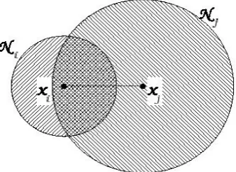
neighborhoods which condition edges in the graph. Neighborhood is different for each object and is computed on the basis of similarities with all other objects. Finally, an edge connects two vertices if they are both contained in the neighborhood of the other one. Figure 1 illustrates the neighborhood con-straint above. In this case, asxiandxj are not both
[image:6.595.103.270.197.318.2]in the intersection, they would not be connected.
Figure 1: To be connected, bothxi andxj must be in the intersection.
3.2 Discovery of Poles
The graph representation helps to discover a set of fully-connected subgraphs (cliques) highly sep-arated, denoted as Poles. BecauseGs(V, E)is built such that two verticesxiandxjare connected if and
only if they are similar11, a clique has the required properties to be a good cluster. Indeed, such a clus-ter guarantees that all its constituents are similar.
The search of maximal cliques in a graph is an NP-complete problem. As a consequence, heuristics are used in order to (1) build a great clique around a starting vertex (Bomze et al., 1999) and (2) choose the starting vertices in such a way cliques are as dis-tant as possible.
Given a starting vertex x, the first heuristic con-sists in adding iteratively the vertexxi which satis-fies the following conditions:
• xiis connected to each vertex inP (withP the
clique/Pole in construction),
• among the connected vertices,xiis the nearest one in average (s(xi, P)).
11
In the sense thatxi(resp. xj) is more similar toxj(resp.
xi) than to other data on average.
As a consequence, initialized withP ={x}, the clique then grows until no vertex can be added.
The second heuristic guides the selection of the starting vertices in a simple manner. Given a set of PolesP1, . . . , Pmalready extracted, we select the
vertexxas in Equation 8.
s(x, P1∪ · · · ∪Pm) = min xi
s(xi, P1∪ · · · ∪Pm) (8)
A new Pole is then built from x if and only ifx
satisfies the following conditions:
• ∀k∈ {1, . . . , m}, x /∈Pk,
• s(x, P1∪ · · · ∪Pm)< s(X, X) = 1
|X|2 X
xi
X
xj
s(xi, xj)
Poles are thus extracted whileP1 ∪ · · · ∪Pm 6= Xand the next starting vertexxis far enough from the previous Poles. In particular, as Poles represent the seeds of the further final clusters, this heuristic gives no restriction on the number of clusters. The first Pole is obtained from the starting pointx∗that checks Equation 9.
x∗= arg min xk∈X
s(xk, X) (9)
3.3 Multi-Assignment
Once the Poles are built, the Pole-Based Overlap-ping Clustering algorithm uses them as clusters rep-resentatives. Membership functions m(., .) are de-fined in order to assign each object to its nearest Poles as shown in Equation 10.
∀xi∈X, Pj∈ {P1, . . . , Pm} : m(xi, Pj) =s(xi, Pj) (10)
For each object xi to assign, the set of poles is
ordered (P1(xi), . . . , Pm(xi)) such that P1(xi)
de-notes the nearest pole12 for xi, P2(xi) the second
nearest pole forxiand so on. We first assignxito its
closest Pole (P1(xi)). Then, for each polePk(xi)(in
the order previously defined) we decide to assignxi
toPk(xi) if it satisfies to the following two
condi-tions :
• ∀k0< k, x
iis assigned toPk0(xi),
• ifk < m,
s(xi, Pk(xi))≥
s(xi, Pk−1(xi)) +s(xi, Pk+1(xi)) 2
This methodology results into a coverage of the starting data set with overlapping clusters (extended Poles).
12
3.4 Hierarchical Organization
A final step consists in organizing the obtained clus-ters into a hierarchical tree. This structure is use-ful to catch the topology of a set of a priori discon-nected groups. The Pole-Based Overlapping Clus-tering algorithm integrates this stage and proceeds by successive merging of the two nearest clusters like for usual agglomerative approaches (Sneath and Sokal, 1973). In this process, the similarity be-tween two clusters is obtained by the average-link (or complete-link) method:
s(Ip, Iq) = 1
|Ip|.|Iq| X
xi∈Ip
X
xj∈Iq
s(xi, xj) (11)
To deal with overlapping clusters we considere in Equation 11 the similarity between an object and it-self to be equal to 1 :s(xi, xi) = 1.
4 Lexical Chaining Algorithm
Once the lexico-semantic knowledge base has been built, it is possible to use it for Lexical Chaining. In this section, we propose a new greedy algorithm which can be seen as an extension of (Hirst and St-Onge, 1997) and (Barzilay and Elhadad, 1997) al-gorithms as it allows polysemous words to belong to different chains thus breaking the “one-word/one-concept per document” paradigm (Gale et al., 1992). Indeed, multi-topic documents like web news sto-ries may introduce different topics in the same doc-ument/url and do not respect the “one sense per dis-course” paradigm. As we want to deal with real-world applications, this characteristic may show in-teresting results for the specific task of Text Summa-rization for Web documents. Indeed, comparatively to the experiments made by (Gale et al., 1992) that deal with “well written discourse”, web documents show unusual discourse structures. In some way, our algorithm follows the idea of (Krovetz, 1998). Finally, it implements (Lin, 1998)’s information-theoretic definition of similarity as the relatedness criterion for the attribution of words to Lexical Chains.
4.1 Algorithm
Our chaining algorithm is based on both approaches of (Barzilay and Elhadad, 1997) and (Hirst and St-Onge, 1997). So, our chaining model is developed
according to all possible alternatives of word senses. In fact, all senses of a word are defined by the clus-ters the word appears in13. We present our algorithm below.
Begin with no chain.
For all distinct nominal units in text order do For all its senses do
a) - among present chains find the sense which satisfies the relatedness criterion and link the new word to this chain.
- Remove unappropriate senses of the new word and the chain members.
b)if no sense is close enough, start a new chain. End For
End For End
4.2 Assignment of a word to a Lexical Chain
In order to assign a word to a given Lexical Chain, we need to evaluate the degree of relatedness of the given word to the words in the chain. This is done by evaluating the relatedness between all the clusters present in the Lexical Chain and all the clusters in which the word appears.
4.2.1 Scoring Function
In order to determine if two clusters are semanti-cally related, we use our lexico-semantic knowledge base and apply (Lin, 1998)’s measure of semantic similarity defined in Equation 12.
simLin(C1, C2) =
2×logP(C0) logP(C1) + logP(C2)
(12)
[image:7.595.331.519.510.665.2]The computation of Equation 12 is illustrated be-low using the fragment of WordNet in Figure 2.
Figure 2: Fragment of WordNet (Lin, 1998).
13
In this case, it would be easy to compute the sim-ilarity between the concepts ofhillandcoastwhere the number attached to each nodeC isP(C). It is shown in Equation 13.
simLin(hill, coast) =2 logP(geological−f ormation)
logP(hill) + logP(coast) = 0.59 (13)
[image:8.595.98.264.262.403.2]However, in our taxonomy, as in any knowl-edge base computed by hierarchical clustering algo-rithms, only leaves contain words. So, upper clusters (i.e. nodes) in the taxonomy gather all distinct words that appear in the clusters they subsume. We present this situation in Figure 3.
Figure 3: Fragment of our taxonomy.
In particular, clusters C305 and C306 of our
hierarchical tree, for the domain of Economy, are represented by the following sets of words
C305 ={life, effort, stability, steps, negotiations}
andC306 ={steps, restructure, corporations, abuse,
interests, ministers}and the number attached to each nodeCisP(C)calculated as in Equation 1414.
P(Ci) =
# of words in the cluster
# of distinct words in all clusters (14)
4.2.2 Relatedness criterion
The relatedness criterion is the threshold that needs to be respected in order to assign a word to a Lexical Chain. In fact, it works like a threshold. In this case, it is based on the average semantic sim-ilarity between all the clusters present in the taxon-omy. So, if all semantic similarities between a candi-date word clusterCkand all the clusters in the chain
∀l, Cl respect the relatedness criterion, the word is
14
The value 2843 in Figure 3 is the total number of distinct words in our concept hierarchy.
assigned to the Lexical Chain. This situation is de-fined in Equation 15 wherecis a constant to be tuned andnis the number of words in the taxonomy. So, if Equation 15 is satisfied, the word wwith cluster
Ckis agglomerated to the Lexical Chain.
∀l, simLin(Ck, Cl)> c× n X
i=0 n X
j=i+1
simLin(Ci, Cj)
n2 2 −n
(15)
In the following section, we present an example of our algorithm.
4.2.3 Example of the Lexical Chain algorithm
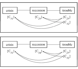
The example below illustrates our Lexical Chain algorithm. Let’s consider that a node is created for the first nominal unit encountered in the text i.e. crisis with its sense (C31). The next
ap-pearing candidate word isrecessionwhich has two senses (C29andC34). Considering a relatedness
cri-terion equal to 0.81 and the following similarities,
[image:8.595.357.496.449.563.2]simLin(C31, C29) = 0.87,simLin(C31, C34) = 0.82, the choice of the sense for recessionsplits the Lexical Chain into two different interpretations as shown in Figure 4, as both similarities overtake the given threshold 0.81.
Figure 4: Interpretations 1 and 2.
The next candidate word trouble has also two senses (C29andC32). As all the words in a
Lexi-cal Chain influence each other in the selection of the respective senses of the new word considered, we have the following situation in Figure 5.
Figure 5: Selection of senses.
only consider this representation or (3) none of the similarities overtake the threshold and we create a new Lexical Chain. So, we proceed with our algo-rithm for both interpretations.
Interpretation 1 shows the following similari-ties simLin(C31, C29) = 0.87, simLin(C31, C32) = 0.75, simLin(C29, C29) = 1.0, simLin(C29, C32) = 0.78 and interpretation 2 the following ones,
simLin(C31, C29) = 0.87, simLin(C31, C32) = 0.75,
simLin(C34, C29) = 0.54,simLin(C34, C32) = 0.55. By computing the average similarities for in-terpretations 1 and 2, we reach the following re-sults: average(Interpretation1) = 0.85 > 0.81 and
average(Interpretation2) = 0.68≯0.81.
As a consequence, the wordtroubleis inserted in the Lexical Chain with the appropriate sense(C29)
as it maximizes the overall similarity of the chain and the chain members senses are updated. In this example, the interpretation with(C32)is discarded
as is the cluster(C34)forrecession. This processing
[image:9.595.89.288.561.615.2]is described in Figure 6.
Figure 6: Selection of appropriate senses.
4.2.4 Score of a chain
Once all chains have been computed, only the high-scoring ones must be picked up as represent-ing the important concepts of the original
docu-ment. Therefore, one must first identify the strongest chains. Like in (Barzilay and Elhadad, 1997), we define a chain score which is defined in Equation 16 where|chain|is the number of words in the chain.
score(chain) =
|chainX|−1
i=0
|chainX|
j=i+1
simLin(Ci, Cj)
(|chain| −1)|chain|
2
(16)
As all chains will be scored, the ones with higher scores will be extracted. Of course, a threshold will have to be defined by the user. In the next section, we will show some qualitative and quantitative re-sults of our architecture.
5 Evaluation
The evaluation of Lexical Chains is generally diffi-cult. Even if they can be effectively used in many practical applications, Lexical Chains are seldom desirable outputs in a real-world application, and it is unclear how to assess their quality indepen-dently of the underlying application in which they are used (Budanitsky and Hirst, 2006). For example, in Summarization, it is hard to determine whether a good or bad performance comes from the efficiency of the lexical chaining algorithm or from the appro-priateness of using Lexical Chains in that kind of application. It is also true that some work has been done in this direction (Budanitsky and Hirst, 2006) by collecting Human Lexical Chains to compare against automatically built Lexical Chains. How-ever, this type of evaluation is logistically impos-sible to perform as we aim at developing a system that does not depend on any language or topic. So, in this section, we will only present some results generated by our architecture (like (Barzilay and El-hadad, 1997; Teich and Fankhauser, 2004) do), al-though we acknowledge that other comparative eval-uations (with WordNet, with Human Lexical Chains or within independent applications like Text Sum-marization) must be done in order to draw definitive conclusions.
We have generated four taxonomies from four dif-ferent domains (Sport, Economy, Politics and War) from a set of documents of the DUC 200415. More-over, we have extracted Lexical Chains for all four
15
domains to show the ability of our system to switch from domain to domain without any problem.
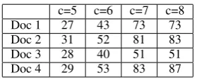
5.1 Quantitative Function
[image:10.595.356.497.70.125.2]Four texts from each domain of the DUC 2004 cor-pus have been used to extract Lexical Chains based on the four knowledge bases built from all texts of DUC 2004 for each one of the four following do-mains: Sport, Economy, Politics and War. However, in this section, we will only present the results from the Sport Domain as results show similar behaviors for the other domains. In particular, we present in Table 1 the characteristics of each document.
# Words #Distinct Words #Distinct Nouns
Doc 1 8133 1956 672
Doc 2 3823 1630 708
Doc 3 4594 953 324
Doc 4 4530 1265 431
Table 1: Characteristics of Documents for Sport
The first interesting conclusion shown in Table 2 is that the number of Lexical Chains does not de-pend on the document size but rather on the nominal units distribution. Indeed, for example, the number of words in Document 1 is twice as big as in Doc-ument 2. Although, we have more Lexical Chains in Document 2 than in Document 1, as Document 2 has more distinct nominal units.
[image:10.595.330.521.255.544.2]c=5 c=6 c=7 c=8 Doc 1 27 43 73 73 Doc 2 31 52 81 83 Doc 3 28 40 51 51 Doc 4 29 53 83 87
Table 2: # Lexical Chains per Document
The second interesting conclusion is that our algo-rithm does not gather words that belong to only one cluster and take advantage of the automatically built lexico-semantic knowledge base. This is illustrated in Table 3. However, it is obvious that by increasing the constantcthe words in a chain tend to belong to only one cluster as it is the case for most of the best Lexical Chains withc= 8.
5.2 Qualitative Evaluation
In this section, as it is done in (Barzilay and Elhadad, 1997; Teich and Fankhauser, 2004), we present the
c=5 c=6 c=7 c=8 Doc 1 19 13 7 7 Doc 2 13 6 3 3
Doc 3 3 4 4 4
Doc 4 6 4 3 3
Table 3: # Clusters per Lexical Chain
five highest-scoring chains for the best threshold that we experimentally evaluated to be c = 7for each domain (See Tables 4, 5, 6, 7). It is clear that the obtained Lexical Chains show a desirable degree of representativeness of the text in analysis.
Domain=Sport, Document=3, c=7
- #0, 1 cluster and score=1.0:{United States, couple, competition}
- #6, 3 clusters and score=1.0:{boats, Sunday night, sailor, Sword, Orion, veteran, cutter, Winston Churchill, Solo Globe, Challenger, navy, Race, sup-position, instructions, responsibility, skipper, east, Melbourne, deck, kilo-meter, masts, bodies, races, GMT, Admiral’s, Cups, Britain, Star, Class, Atlanta, Seattle, arms, fatality, sea, waves, dark, yacht’s, Dad, Guy’s, son, Mark, beer, talk, life, Richard, Winning, affair, canopy, death}
- #9, 1 cluster and score=1.0:{record, days, hours, minutes, rescue}
- #16, 3 clusters and score=1.0: {Snow, shape, north, easters, thunder, storm, change, knots, west, level, maxi’s, search, Authority, seas, helicopter, night vision, equipment, feet, rescues, Campbell, suffering, hypothermia, safety, foot, sailors, colleagues, Hospital, deaths, bodies, fatality}
- #19, 2 clusters and score=1.0:{challenge, crew, Monday, VC, Offshore, Stand, Newcastle, mid morning, Eden, Rescuers, aircraft, unsure, where-abouts, killing, contact}
Table 4: 5 best Lexical Chains for Sport
Domain=Economy, Document=5, c=7
- #88, 4 clusters and score=1.0:{sign, chance, Rio, Janeiro, Grande, Sul, uphill, promise, hospitals, powerhouse, success, inhabitants, victory, pad, presidency, contingent, exit, legislature}
- #50, 1 cluster and score=1.0:{transactions, taxes, Stabilization, spate, fuel, income, fortunes, means}
- #77, 1 cluster and score=1.0:{proposal, factory, owners, Fund, Rubin’s}
- #126, 1 cluster and score=1.0:{disaster, control, investment, review}
- #12, 2 clusters and score=0.99:{issue, order, University, population, ques-tion, timing, currencies}
Table 5: 5 best Lexical Chains for Economy
For instance, the Lexical Chain #16 in the domain of Sport clearly exemplifies the tragedy of climbers that were killed in a sudden change of weather in the mountains and who could not be rescued by the authorities.
[image:10.595.76.295.256.311.2] [image:10.595.116.256.465.522.2]Domain=Politics, Document=3, c=7
- #5, 1 cluster and score=1.0:{report, leaders, lives, information}
- #33, 1 cluster and score=1.0:{past, attention, defenders, investigations}
- #28, 2 clusters and score=0.95:{investigators, hospital, ward, wounds, neck, description, fashion, suspects, raids, assault, rifles, door, further de-tails, surgery, service, detective, Igor, Kozhevnikov, Ministry}
- #40, 2 clusters and score=0.92:{security, times, weeks, fire}
- #24, 3 clusters and score=0.85:{enemies, Choice, stairwell, assailants, woman, attackers, entrance, car, guns, Friends, relatives, Mrs. Staravoitova, founder, movement, well thought, Sergei, Kozyrev, Association, Societies, supporter, Stalin’s, council, criminals, Yegor, Gaidar, minister, ally, sugges-tions, measures, smile, commitment}
Table 6: 5 best Lexical Chains for Politics
Domain=War, Document=1, c=7
- #25, 2 clusters and score=1.0: {lightning, advance, Africa’s, nation, outskirts, capital Kinshasa, troops, Angola, Zimbabwe, Namibia, chunk, routes, Katanga, Eastern, Kasai, provinces, copper}
- #53, 1 cluster and score=1.0:{Back, years, Ngeyo, farm, farmers, organi-zation, breadbasket, quarter, century, businessman, hotels, tourist, memory, rivalry, rebellions}
- #56, 1 cluster and score=1.0:{political, freedoms, Hutus, Mai-Mai, war-riors, Hunde, Nande, militiamen, Rwanda, ideology, weapons, persecu-tion, landowners, ranchers, anarchy, Safari, Ngezayo, farmer, hotel, owner, camps}
- #24, 2 clusters and score=0.87: {fighting, people, leaders, diplomats, cause, president, Washington, U.S, units, weeks}
- #51, 2 clusters and score=0.82:{West, buildings, sight, point, tourists, mountain, gorillas, shops, guest, disputes}
Table 7: 5 best Lexical Chains for War
to express any idea about Politics. Moreover, due to the small number of inter-related nominal units within the Lexical Chain, this one can not be under-stood as it is without context. In fact, it was related to problems of car firing that have been occurring in the past few weeks and provoked security problems in the town.
Although some Lexical Chains are understand-able as they are, most of them must be replaced in their context to fully understand their representative-ness of the topics or subtopics of the text being an-alyzed. As a consequence, we deeply believe that Lexical Chains must be evaluated in the context of Natural Language Processing applications (such as Text Summarization (Doran et al., 2004)), as com-paring Lexical Chains as they are is a very difficult task to tackle which may even lead to inconclusive results.
6 Conclusions and Future Work
In this paper, we implemented a greedy Language-Independent algorithm for building Lexical Chains.
For that purpose, we first constructed a lexico-semantic knowledge base by applying the Pole-Based Overlapping Clustering algorithm (Cleuziou et al., 2004) to word-context vectors obtained by the application of the SCP(., .) measure (Silva et al., 1999) and theInf oSimBA(., .) (Dias and Alves, 2005) similarity measure. In a second step, we im-plemented (Lin, 1998)’s similarity measure and used it to define the relatedness criterion in order to as-sign a given word to a given chain in the lexical chaining process. Finally, our experimental eval-uation shows that relevant Lexical Chains can be constructed with our lexical chaining algorithm, al-though we acknowledge that more comparative eval-uations must be done in order to draw definitive con-clusions. In particular, in future work, we want to compare our methodology using WordNet as the ba-sic knowledge base, implement different similarity measures (Resnik, 1995; Jiang and Conrath, 1997; Leacock and Chodorow, 1998), experiment differ-ent Lexical Chains algorithms (Hirst and St-Onge, 1997; Barzilay and Elhadad, 1997; Galley and McK-eown, 2003), scale our greedy algorithm for real-world applications following (Silber and McCoy, 2002) ideas and finally evaluate our system in inde-pendent Natural Language Processing applications such as Text Summarization (Doran et al., 2004).
References
R. Barzilay and M. Elhadad. 1997.Using Lexical Chains for Text Summarization. Proceedings of the Intelli-gent Scalable Text Summarization Workshop (ISTS-97), ACL, Madrid, Spain, pages 10-18.
I. Bomze, M. Budinich, P. Pardalos, and M. Pelillo. 1999. The Maximum Clique Problem. Handbook of Com-binatorial Optimization, volume 4. Kluwer Academic publishers, Boston, MA.
T. Brants. 2000. TnT - a Statistical Part-of-Speech Tag-ger. In Proceedings of the 6th Applied NLP Confer-ence, ANLP-2000. Seattle, WA.
A. Budanitsky and G. Hirst. 2006.Evaluating WordNet-based Measures of Lexical Semantic Relatedness. In Computational Linguistics, 32(1). pages: 13-47.
G. Cleuziou, L. Martin, and C. Vrain. 2004. PoBOC: an Overlapping Clustering Algorithm. Application to Rule-Based Classication and Textual Data. In Pro-ceedings of the 16th European Conference on Artifi-cial Intelligence, pages 440-444, Spain, August 22-27.
G. Cleuziou, V. Clavier, L. Martin. 2003. Une M´ethode de Regroupement de Mots Fond´ee sur la Recherche de Cliques dans un Graphe de Cooccurrences. In Pro-ceedings of Rencontres Terminologie et Intelligence Artificielle, France. pages 179-182.
B. Daille. 1995. Study and Implementation of Combined Techniques for Automatic Extraction of Terminology. In The balancing act combining symbolic and statisti-cal approaches to language. MIT Press.
G. Dias and E. Alves. 2005. Unsupervised Topic Seg-mentation Based on Word Co-occurrence and Multi-Word Units for Text Summarization. In Proceedings of the ELECTRA Workshop associated to 28th ACM SIGIR Conference, Salvador, Brazil, pages 41-48.
G. Dias, S. Guillor´e and J.G.P. Lopes. 1999. Language Independent Automatic Acquisition of Rigid Multi-word Units from Unrestricted Text Corpora. In Pro-ceedings of 6th Annual Conference on Natural Lan-guage Processing, Carg`ese, France, pages 333-339.
W. Doran, N. Stokes, J. Carthy and J. Dunnion. 2004. Assessing the Impact of Lexical Chain Scoring Meth-ods and Sentence Extraction Schemes on Summariza-tion. In Proc. of the 5th Conference on Intelligent Text Processing and Computational Linguistics.
V. Estivill-Castro, I. Lee, and A. T. Murray. 2001. Crite-ria on Proximity Graphs for Boundary Extraction and Spatial Clustering. In Proceedings of the 5th Pacific-Asia Conference on Knowledge Discovery and Data Mining, Springer-Verlag. pages 348-357.
C.D. Fellbaum. 1998. WordNet: An Electronic Lexical Database. MIT Press, New York.
W. Gale, K. Church, and D. Yarowsky. 1992.One Sense per Discourse. In Proceedings of the DARPA Speech and Natural Language Workshop.
M. Galley and K. McKeown. 2003. Improving Word Sense Disambiguation in Lexical Chaining. In Pro-ceedings of 18th International Joint Conference on Ar-tificial Intelligence (IJCAI’03), Acapulco, Mexico.
G. Hirst and D. St-Onge. 1997.Lexical Chains as Repre-sentation of Context for the Detection and Correction of Malapropisms. In WordNet: An electronic lexical database and some of its applications. MIT Press.
J.W. Jaromczyk and G.T. Toussaint. 1992. Relative Neighborhood Graphs and Their Relatives. P-IEEE, 80, pages 1502-1517.
J.J. Jiang and D.W. Conrath. 1997. Semantic Similarity Based on Corpus Statistics and Lexical Taxonomy. In Proceedings of International Conference on Research in Computational Linguistics, Taiwan.
R. Krovetz. 1998. More than One Sense per Discourse. NEC Princeton NJ Labs., Research Memorandum.
C. Leacock and M. Chodorow. 1998. Combining Local Context and WordNet Similarity for Word Sense Iden-tification. In C. Fellbaum, editor, WordNet: An elec-tronic lexical database. MIT Press. pages 265-283.
D. Lin. 1998. An Information-theoretic Definition of Similarity. In 15th International Conference on Ma-chine Learning. Morgan Kaufmann, San Francisco.
G. Miller. 1995.WordNet: An Lexical Database for Eng-lish. Communications of the Association for Comput-ing Machinery (CACM), 38(11), pages 39-41.
J. Morris and G. Hirst. 1991. Lexical Cohesion Com-puted by Thesaural Relations as an Indicator of the Structure of Text. Computational Linguistics, 17(1).
P. Pantel and D. Lin. 2002. Discovering Word Senses from Text. In Proceedings of the Eighth ACM SIGKDD International Conference on Knowl-edge Discovery and Data Mining. pages 613-619.
P. Resnik. 1995. Using Information Content to Evaluate Semantic Similarity. In Proceedings of the 14th In-ternational Joint Conference on Artificial Intelligence, Montreal. pages 448-453.
P.M. Roget. 1852. Roget’s Thesaurus of English Words and Phrases. Harlow, Essex, England: Longman.
G. Salton, C.S. Yang and C.T. Yu. 1975. A Theory of Term Importance in Automatic Text Analysis. In American Society of Information Science, 26(1).
G. Silber and K. McCoy. 2002. Efficiently Computed Lexical Chains as an Intermediate Representation for Automatic Text Summarization. Computational Lin-guistics, 28(4), pages 487-496.
J. Silva, G. Dias, S. Guillor´e and J.G.P. Lopes. 1999. Us-ing LocalMaxs Algorithm for the Extraction of Con-tiguous and Non-conCon-tiguous Multiword Lexical Units. In Proceedings of 9th Portuguese Conference in Arti-ficial Intelligence. Springer-Verlag.
P. H. A. Sneath and R. R. Sokal. 1973.Numerical Taxon-omy - The Principles and Practice of Numerical Clas-sification. San Francisco, Freeman and Co.