Actively Private and Correct MPC Scheme in t
<
n
/
2
from Passively Secure Schemes with Small Overhead
Dai IKARASHI, Ryo KIKUCHI, Koki HAMADA, and Koji CHIDA
NTT Corporation,
{ikarashi.dai, kikuchi.ryo, chida.koji, hamada.koki}@lab.ntt.co.jp
Abstract. Recently, several efforts to implement and use an unconditionally secure multi-party computation (MPC) scheme have been put into practice. These implementations are passively secure MPC schemes in which an adversary must follow the MPC schemes. Although passively secure MPC schemes are efficient, passive security has the strong restriction concerning the behavior of the adversary. We investigate how secure we can construct MPC schemes while maintaining comparable efficiency with the passive case, and propose a construction of an actively secure MPC scheme from passively secure ones. Our construction is secure in the t<n/2 setting, which is the same as the passively secure one. Our construction operates not only the theoretical minimal set for computing arbitrary circuits, that is, addition and multiplication, but also high-level operations such as shuffling and sorting. We do not use the broadcast channel in the construction. Therefore, privacy and correctness are achieved but robustness is absent; if the adversary cheats, a protocol may not be finished but anyone can detect the cheat (and may stop the protocol) without leaking secret information. Instead of this, our construction requires O((cBn+n2)κ) communication that is comparable to one of the
best known passively secure MPC schemes, O((cMn+n2) log n), whereκdenote the security parameter, cBdenotes the sum of multiplication gates and high-level operations, and cMdenotes the number of multiplication gates. Furthermore, we implemented our construction and confirmed that its efficiency is comparable to the current fastest passively secure implementation.
Keywords: Multi-party computation, Unconditional security, Active adversary
1
Introduction
Multi-party computation (MPC) is a technique that enables parties with inputs to evaluate a function on the inputs while keeping them secret. MPC has been a central themes of cryptographic study because of its applicability and generality, and MPC theory was developed in the period from the mid-1980s to the mid-2000s, Recently, some sophisticated method-ologies to construct MPC schemes have been developed. These includes hardware that is much more efficient than that of decades ago, and MPC schemes that efficiently compute “high-level” operations such as bit-decomposition, shuffling and sorting. Thus, several efforts to implement and use MPC have been put into practice [5, 6, 18]. The (k,n)-threshold
uncon-ditionally secure MPC is the most frequently used MPC scheme since it is more efficient compared with other schemes. It requires no heavy operations that require milliseconds such as modular exponentiations.
Let n and t denote the number of parties and corrupted parties, respectively. Most MPC implementations for practical use, including the above, are secure against a passive adversary regarding corruption of the t < n/2 setting, i.e., they are secure against the adversary that follows an MPC scheme with honest majority. Although active security, where the adversary can carry out arbitrary behavior, can be achieved, passively secure MPC schemes are much more efficient than actively secure ones, and the current practical results have been passive secure.
However, passive security requires a somewhat strong restriction concerning the behavior of the adversary. Therefore, it should be motivated to replace passively secure MPC schemes to more secure (active) ones for practical use. In other words, “How secure can we construct MPC schemes while maintaining comparable efficiency to passive ones?”. If we
aim to use actively secure MPC schemes in practice the same way we do passively secure ones, the following three points need to be satisfied. First, the amount of communication should be small and comparable to the passive setting, which is O(cMn log n+n2log n) [12], where cM is the number of multiplication gates. The communication cost is the
Table 1. Comparison of current circuit-based MPC protocols
Adversary Robustness Threshold Communication (bits) Building blocks Security HM01 [16] active yes t<n/3 O(cMn2κ)+poly(nκ) algebraic circuit unconditional DN07 [12] active yes t<n/3 O(cMn log n+dMn2log n)+poly(nκ) algebraic circuit unconditional
BH08 [2] active yes t<n/3 O(cMn log n+dMn2log n+n3log n) algebraic circuit perfect CDD+99 [8] active yes t<n/2 O(cMn5κ+n4κ)+O(cMn4κ)BC algebraic circuit unconditional
BH06 [1] active yes t<n/2 O(cMn2κ+n5κ2)+O(n3κ)BC algebraic circuit unconditional BFO12 [3] active yes t<n/2 O(cM(nϕ+κ)+dMn2κ+n7κ)+O(n3κ)BC algebraic circuit unconditional Ours active no t<n/2 O((cBn+n2)κ) passively secure MPC unconditional DN07 [12] passive - t<n/2 O((cMn+n2) log n) algebraic circuit perfect “Active” means an adversary can do arbitrary things, “passive” means the adversary must follow the protocol, “yes” means the protocol must be finished whatever the adversary does, “no” means the protocol may not be finished while the parties can detect and stop the protocol without leaking secret information, t is the number of corrupted parties, n is the number of all parties,
cMis the number of multiplication gates of the circuit, dM is the multiplicative depth of the circuit, xBCmeans that x bits are communicated via the broadcast channel, cBis the number of building blocks that consist of multiplication gates and high-level operations. Note that in Ref. [8], there are two descriptions of O(n4) and O(n5) communication via broadcast. The correct one is
the former.
1.1 Related Works and Our Results
There have been studies on the communication cost for actively secure MPC schemes that compute algebraic circuits. We list some studies in Table 1. Regarding t <n/3, Damgård and Nielsen [12] and Beerliov´a-Trub´ıniov´a and Hirt [2] proposed unconditional and perfect MPC schemes. Their schemes require a small communication cost that is comparable to passively secure ones but they tolerate smaller corruptions. Regarding t < n/2, Beerliov´a-Trub´ıniov´a and Hirt [1] proposed an actively secure MPC scheme with O(cMn2κ+n5κ2)+O(n3κ)BCcommunications, and Ben-Sasson et al. [3]
also proposed a scheme with O(cM(nϕ+κ)+dMn2κ+n7κ)+O(n3κ)BCcommunications, where κ denotes a security
parameter, dM denotes the multiplicative depth of the circuit,ϕis a larger element either a field size or log n, andBC
denotes a broadcast channel. The broadcast channel is a communication channel that guarantees that “all recipients are convinced that all other parties receive the same data that they received.” To our knowledge, the broadcast channel costs
O(n3) communication at least [17] and requires trusted setup in the t<n/2 setting. Therefore, the communication cost of
the above two schemes can be regarded as O(cMn2κ+n5κ2+n6κ) and O(cM(nϕ+κ)+dMn2κ+n7κ), respectively. If the
circuit is large, i.e., cMis much larger than n7, and “wide”, i.e., dMis much smaller than cM, the amortized communication
complexity of Ben-Sasson et al. ’s scheme is O(n log n) per multiplication, which is the same as the best passively secure MPC scheme [12].
The above studies mainly focused on the theory of MPC, which is insufficient for practice use. The circuit is not always very large or wide, and the effect of a high-dimensional factor in the communication cost such as O(n7κ) cannot
be ignored Furthermore, the MPC scheme that computes a high-level operation, for example, bit-decomposition [11], shuffling [21], or sorting [15], is useful for efficient MPC execution, but the above results only support an algebraic circuit as a building block.
One of the main causes of a high-dimensional factor in communication is the broadcast channel. Therefore, it is natural that one attempts to construct an actively secure MPC scheme without the broadcast channel. There has been much less progress in the direction of constructing actively secure without the broadcast channel regarding the t < n/2 setting. One of the reason for this is that in this setting, robustness cannot be achieved. Robustness guarantees that “an MPC scheme must be finished correctly whatever an adversary does”. However, even in the t <n/2 setting, an MPC scheme can achieve correctness and privacy, which guarantee that if the adversary cheats, everyone can detect it (and may stop the protocol) without leaking secret information. To achieve the objective of constructing an actively secure MPC scheme while maintaining the efficiency of a passively secure one, this setting is worth studying.
From the viewpoint of high-level operation, current MPC schemes that compute high-level operations were designed in the paradigm of computing on shared values. In this paradigm, secret values are preliminarily shared with a secret-sharing scheme to all parties that participate in the MPC schemes. Then the MPC schemes take secretly shared values as inputs from each party and output the result in secretly shared form. Therefore, if we generally use MPC schemes in this paradigm as building blocks for constructing an actively secure MPC scheme, many high-level operations can be used.
We propose a construction of a non-robust, actively and unconditionally secure MPC scheme in the t < n/2 set-ting without the broadcast channel while maintaining efficiency comparable to a passively secure one. Our scheme also achieves comparable communication complexity, O((cBn+n2)κ), where cBis the number of building blocks consisting of
first actively secure MPC scheme that has no assumption in the t<n/2 setting since the current results uses the broadcast channel that implicitly requires a trusted setup.
1.2 Brief Explanation of Our Construction
At the start of the protocol, each party has its own input. The parties distribute their inputs through (k,n) threshold
secret-sharing, and then check the consistency of the shares. Consistency means that for any subset that contains k honest parties, the revealed values are the same. It is known that the consistency can be easily batch checked if a negligible error is allowed by using a plain randomness and random share. A more detailed description can be found in Appendix G.
Each party has consistent shares at this time. This situation is the same in the paradigm of computing on shared values. We perform a protocol to compute a function by using passively secure MPC schemes as building blocks. More precisely, our scheme takes the following three phases.
Randomization Phase: This phase converts shares into randomized shared pairs to prevent an adversary from tampering
with shared values. Intuitively speaking, the Randomization Phase generates the shares that can be seen as a MAC or checksum of shared values. In the simplest case, this phase changes ([[ a ]]) to ([[ a ]],[[ ra ]]) and stores [[ r ]], where r is uniformly at random and unknown for any party. We formalize it in general as follows. A randomized shared pair is formed as a pair of an element on a ringX, which parties use to conduct computation, and an element ofX-algebra
Y. Namely, in the simplest case, [[ a ]] belongs toXand [[ ra ]] belongs toY. This generalization makes it possible to use our construction on not only a field but also a ring, as used in [10], and even if the size ofXis small, our scheme is secure by enlargingY.
Computation Phase: This phase computes the target function redundantly onX andY. We denote a simple case as
an example. Let F = f1◦ f2be the target function,Πf1, Πf2 be MPC schemes that are designed in the paradigm of
computing on shared values, and ([[ a ]],[[ ra ]]) be input. The Computation Phase first computes ([[ f2(a) ]],[[ r f2(a) ]])
from ([[ a ]],[[ ra ]]) viaΠf2then computes ([[ f1◦ f2(a) ]],[[ r( f1◦ f2)(a) ]])=([[ F(a) ]],[[ rF(a) ]]) viaΠf1. Constitutive
(passively secure) MPC schemes,Πf1, Πf2, should satisfy two properties. The first is the operation onY-distribution,
i.e.,Πf2 can compute from ([[ a ]],[[ ra ]]) to ([[ f2(a) ]],[[ r f2(a) ]]). The second is tamper-simulatability, which means
“An adversary’s ability to tamper with the results of the protocol is restricted to the addition of values he/she knows”. This second property is needed in the next phase. As long as the above two conditions hold,Πf1, Πf2are arbitrary so
we use not only multiplication but also high-level operations.
Proof Phase: This phase determines if a computation has been cheated. The results of the computation are all checked at
once by proving that the results onXandYare “equal”. In the above example, the parties reveal
[[ r ]](ρ1[[ a ]]+ρ2[[ f2(a) ]]+ρ3[[ F(a) ]])−(ρ1[[ ra ]]+ρ2[[ r f2(a) ]]+ρ3[[ rF(a) ]])
and check if it is 0 or not, whereρi is uniformly at random for i ={1,2,3}. If the adversary changes from [[ a ]] to
[[ a+δ]], this equation does not hold except with negligible probability since tamper-simulatability guarantees that
δis known to an adversary (and it inherently says thatδdoes not depends on r). The concentration of all proofs on one element ofYmakes the proof very efficient and reduces the number of times unnecessary information can be revealed.
As a result of the above phases, each player has the share of output [[ F(a) ]]. The parties perform an actively secure reveal protocol (described in Appendix G) and obtain the result.
1.3 Paper Organization
In Section 2, we introduce known tools and the notations used in the paper, and in Section 3, we explain the building blocks of our construction. In Section 4, we propose our construction that involves converting passive MPC schemes to an active one. In Section 5, we describe the experimental results to demonstrate the practical efficiency of our construction.
2
Preliminaries
We introduce some preliminaries, an algebra that is an algebraic structure used in our construction, our notations, and the passive unconditionally secure MPC protocols used in the examples of our construction.
2.1 Algebra
Definition 1. (X-algebra)
A ringYis called anX-algebra if there exist another ringXand an operation, scalar multiplication, betweenXandY that satisfies the following condition for any x,x′∈ Xand y,y′∈ Y.
x(y+y′)=xy+xy′,(x+x′)y=xy+x′y,(xx′)y=x(x′y),1Xy=y
Example 1. For any fieldF, its extensionE(F)d with arbitrary positive integer d is anF-algebra, where scalar
multipli-cation betweenF andE(F)dis xy=(xy
0,· · · ,xyd−1) for any x∈ F and y∈ E(F)d.
2.2 Secret Sharing
We use the (k,n) threshold secret sharing scheme; a secret is separated into n pieces called shares and sent to parties.
Parties can then reveal the secret from k or more shares. We assume a secret sharing scheme is Shamir’s on a field, or a replicated secret sharing scheme on a field/ring. However, another secret sharing scheme that satisfies the following requirements can be used instead.
– Perfect privacy: the joint distribution of any k−1 shares does not depend on the secret. – Uniqueness of shared value: any k shares determines a unique shared value.
– Existence of mandatory building blocks: there are MPC protocols called mandatory building blocks, described later in Section 3. Roughly speaking, we require passively secure scalar multiplication, scalar sum-product, addition/subtraction, and actively secure random number generation and revealing in the secret sharing scheme.
Note that uniqueness of a shared value implies the existence of the share regeneration algorithm, which computes a share from other k shares. Of course, Shamir’s and replicated secret sharing schemes satisfy the above requirements. For example, Shamir’s satisfies the second condition since k shares uniquely determine the k−1 polynomial onF.
Additionally, we say a (k,n) threshold secret sharing scheme is an LSSS (Linear Secret Sharing Scheme) if both the
reconstruction and the share regeneration of the scheme are represented by linear combinations of field/ring elements in shares with fixed coefficients. Shamir’s and replicated secret sharing schemes are both LSSS.
2.3 Common Structures and Notations
We use the following structures in this paper.
– X: An arbitrary ring on which parties wish to conduct their computation – Y: AnX-algebra
– F: An arbitrary field as an example of rings
– E(F)d: A d-degree extension field ofF for some positive integer d as an example ofF-algebras
– Xr:{ar∈ Y |a∈ X}for some r∈RY
Additionally, we use the following notations in this paper.
– “Share” and “shared value” denote each party’s share and the tuple of shares of all parties, respectively. Shares of a shared value x are denoted by [[ x ]].
– A share of a shared value x for a party Piis denoted by [[ x ]]i, and ones for a subset of partiesQare denoted by [[ x ]]Q.
– [[X]] denotes the set of arbitrary shared values ofX. – ⟨⟨ Xr⟩⟩denotes [[X]]×[[Xr ]].
– ⟨⟨a⟩⟩r(or⟨⟨a⟩⟩) denotes ([[ a ]],[[ ar ]])∈ ⟨⟨ Xr⟩⟩.
– t, k, and n denote the number of corrupted parties, the threshold of the secret sharing scheme, and the number of parties, respectively. Note that k=t+1.
– F, m, andµdenote the function that parties compute, the number of inputs of F, and the number of outputs of F, respectively.
2.4 Known Protocols used in Passive Setting
Our construction is a conversion to an active scheme from passive schemes; thus, we require protocols in the passive scheme, that is, random number generation, multiplication, and reveal.
Random Number Generation A random number generation (RNG) protocol creates a shared value whose plaintext is
uniformly random inX. If one allows the security of pseudorandom numbers, pseudorandom secret sharing [9], which realizes an RNG protocol with no communication, can be used. Otherwise, RNG using a Van der Monde matrix with the
Passive Multiplication Multiplication is the main protocol in most MPC schemes because addition tends to be involved
in the homomorphism of the underlying secret sharing scheme or encryption; thus, multiplication is sufficient to compute arbitrary circuits. Unlike RNG, there is no multiplication protocol that satisfies efficiency, active security, and simplicity, especially in the t<n/2 setting.
We introduce two protocols: GRR-(passive) multiplication [13] and DN-(passive) multiplication [12]. They are de-scribed in detail in Appendix A. Both protocols are based on Shamir’s secret sharing. They are passive protocols; however, they have a certain weak tamper-resistance as we will discuss in Section 3. GRR-multiplication is O(n2) communication and one round, and DN-multiplication is O(n) communication and two rounds. When t is small (e.g., t = 1), GRR-multiplication is better in terms of not only round efficiency, but also communication efficiency thanks to its small constant coefficient.
Reveal The reveal protocol reconstructs a shared value and publishes the reconstructed plaintext to all parties. Although
there are O(n) passive reveal protocols [12], a reveal protocol in our construction requires correctness against an active adversary. Note that the correct reveal protocol is used only once in the Proof Phase, and passively secure protocols are allowed in other parts such as the sub-protocol of DN-multiplication in the Computation Phase. An example of a correct reveal protocol in Shamir’s secret sharing scheme is given in Appendix A. This costs O(n2) communications and two
rounds.
Passive Shuffling Protocol Recently, the shuffling operation has come to be recognized as a significant operation in
MPC. It can be used for data filtering [21] and sorting [15]. Although the shuffling operation can be realized as a logical circuit, it is quite heavy. Therefore, more efficient shuffling protocols have been proposed by Laur et al. [21].
They proposed passive and active protocols. The passive protocols are t<n/2 protocols. However, the active protocols are t<n/3 protocols. Our construction can convert a passive protocol into a t<n/2 non-robust one.
3
Available Building Blocks
In this section, we introduce passive MPC protocols used in our construction as building blocks, and we also introduce the two required conditions for them, tamper-simulatability andY-distribution. The building blocks are separated into the
following two types.
1. Mandatory building blocks, which constitute the two phases of our construction: the Randomization Phase and the Proof Phase. They are required regardless of the function F that parties wish to compute. Mandatory building blocks should satisfy tamper-simulatability, which restricts the adversary’s ability to cheat as only the addition of known values. (Only one reveal requires active correctness by itself.)
2. Optional building blocks, which are selectively used and constitute the Computation Phase. Parties can construct the circuit that realizes the desired function F through composition of optional building blocks. Optional building blocks should satisfy tamper-simulatability and the existence ofY-distribution, which are their realization on theX-algebra Y.
Readers might assume that the two conditions limit the generality of our construction; however, we show that these conditions are quite easy to satisfy for various well-known primitive operations in unconditionally secure MPC schemes.
3.1 Tamper-Simulatability
In our construction, all building blocks require tamper-simulatability, which is a kind of weak tamper-resistance and means that “an adversary’s ability to tamper with the results of the protocol is restricted to the addition of values he/she knows.” From the viewpoint of correctness, this property provides the following benefit. In the first phase, namely, the randomization Phase, each input [[ a ]]∈ [[X]] is converted into a randomized shared pair ([[ a ]],[[ ar ]])∈ [[X]]×[[Y]] by multiplying [[ r ]], where r ∈ Yis a random value that no party knows, and in the following Computation Phase, all computations are conducted in the form of randomized shared pairs. Tamper-simulatability guarantees that even if the adversary tampers with a randomized shared value ([[ a ]],[[ ar ]]) to ([[ a′]],[[ b′]]), a′and b′are always represented as a+x
and ar+y using x and y, which are independent of r. Therefore, honest parties can detect the existence of tampering by
testing whether r(a+x)−(ra+y)(=rx−y)=0 holds, since rx−y is random for the adversary and he/she cannot force it to be zero.
Tamper-simulatability is defined for protocols whose inputs and outputs are in secret-shared form. We call the dif-ference between a legitimate output and a tampered output tamper-difference (i.e., when the adversary tampers with a
shared value [[ f (a) ]] to [[ f (a)+x ]], the tamper-difference is x). We define tamper-simulatability in the manner that for any adversary, there exists a simulator who has only the same information as the adversary, and he/she can compute the tamper-difference.
Definition 2. (tamper-simulatability)
LetΠf be a protocol that realizes the function f : Xm → Xµ, [[→−a ]] = ([[ a0]], . . . ,[[ am−1]]) be inputs ofΠf, [[
− →
b ]] =
([[ b0]], . . . ,[[ bµ−1]]) be the legitimate outputs of the function f ([[→−a ]]), and [[
− →
b′]] = ([[ b′0]], . . . ,[[ b′µ−1]]) be the actual
(possibly tampered with) outputs ofΠf conducted with an active adversary. We say thatΠf has tamper-simulatability if
and only if, for any adversary with any auxiliary input aux, there exists a simulatorSthat satisfies
Pr [
−
→e ← S(aux,[[→−a ]]
I,[[→−b′]]I,ViewI,RI) :→−e =→−b −→−b′
] =1,
where→−b −→−b′is a pair-wise subtraction onX, and ViewI andRI are the protocol’s view and random tapes of corrupted parties, respectively.
(Linear-Combinatorial Protocols)
We consider a class of MPC protocols we call linear-combinatorial protocols. Protocols in this class consist of the fol-lowing two phases.
1. First, in the offline phase, each party locally computes his/her inputs of the next online phase from his/her inputs by arbitrary functions.
2. Then, in the online phase, each party interacts with other parties freely except that in each round, the party sends only linear combinations of the outputs of the offline phase and received data, where coefficients of the linear combinations are public.
In fact, the class of linear-combinatorial protocols is quite general and contains various primitive protocols frequently used in unconditionally secure MPC schemes such as random number generation, multiplication, reveal, and resharing. (Note that any offline protocols including addition belong to the class of linear-combinatorial protocols since the offline phase allows arbitrary local computations.)
The other significant fact is that any linear-combinatorial protocols on LSSS are tamper-simulatable. Due to space limitations, we give the proof and the formal definition of linear-combinatorial protocols in Appendix B.
Theorem 1. (informal) Any linear-combinatorial protocols are tamper-simulatable.
Corollary 1. GRR-multiplication, DN-multiplication, DN-RNG, and resharing are all tamper-simulatable.
Next, we claim that parallel execution preserves tamper-simulatability. Parallel execution is a concurrent composition of protocols, where each protocol’s inputs of honest parties do not depend on the outputs of the other protocols. Intuitively speaking, parallel execution represents that constitutive protocols are executed simultaneously. Note that parallel execution does not include so-called sequential composition.
Lemma 1. (closure of tamper-simulatability on independent compositions)
Parallel execution of unconditionally secure tamper-simulatable protocols is tamper-simulatable.
The proof is given in Appendix C.
3.2 Mandatory Building Blocks
The mandatory building blocks are the following seven operations consisting of a uniform RNG, four algebraic operations onY, and reveal and synchronization (only in an asynchronous setting). They are used in the Randomization Phase and the Proof Phase to guarantee the correctness of the computation.
1. RNG: [[ r ]]←RANDY
2. scalar multiplication: [[ ar ]] for [[ a ]]∈[[X]] and [[ r ]]∈[[Y]] 3. scalar product-sum: [[∑
i<d
airi]] for d∈N, [[ a0]],· · ·,[[ ad−1]]∈[[X]] and [[ r0]],· · ·,[[ rd−1]]∈[[Y]]
4. addition/subtraction on [[Y]] 5. multiplication on [[Y]]
6. correct reveal of shared value on [[Y]]
7. synchronization: the protocol SYNC to simulate the synchronous setting
Simulating Synchronous Setting in Asynchronous Setting SYNC (Scheme 1) is a protocol to simulate the
asyn-chronous setting and forces honest parties to wait to receive all data before SYNC.
Scheme 1 [Protocol] SYNC Input: none
Output: none
1: for each party P do
2: P waits to receive all data before this protocol.
3: If P has received all data, P sendsϕto all other parties.ϕis arbitrary fixed data. 4: for each party P do
5: P waits to receiveϕfrom all other parties.
6: If P has receivedϕfrom all other parties, P proceeds to the next protocol.
3.3 Optional Building Blocks
Optional building blocks are protocols that realize primitive operations in the computation phase. In theory, addition and multiplication are sufficient for computing arbitrary functions. Additionally, our construction allows us to add arbitrary functions that satisfy certain conditions. For function f and its MPC protocolΠf, f can be used in the Computation Phase
in our construction if f andΠfsatisfy the following conditions.
Condition 1 (conditions of optional building blocks)
1. Πf is tamper-simulatable
2. There exists a tamper-simulatableY-distribution protocolΠf′of f
Roughly speaking,Y-distribution represents the existence of a protocol that computes the function f onE(F)d.
Definition 3. (Y-distribution)
Let f :Xℓ → Xmbe anℓ-input m-output building block function on a ringX, and letYandZbe anX-algebra and a
direct product ringX × Y, respectively. We say a function f′:Zℓ× Y → Ymis aY-distribution of f if for any (→−a )∈ Xℓ
and r∈ Y, f′satisfies f′(→−a,→−a r,r)=f (→−a )r, where→−a r denotes (a0r,· · ·,aℓ−1r).
We call a protocol that realizes f′ a Y-distribution protocol of f . In contrast withY-distribution, a protocol that realizes f is called a passive protocol of f .
For example, with a field,F, asXand its extensionE(F)d with an arbitrary positive integer d, asY, linear transfor-mations including addition, multiplication, and resharing have theirE(F)d-distributions, as shown in Appendix E.
4
Proposed Construction
In this section, we explain our construction, which consists of three phases: Randomization, Computation, and Proof. We describe these three phases and the overall construction. Then, we analyze the security, that is, privacy and correctness, of the construction. At the end of this section, we analyze the communication efficiency and the round efficiency of the construction.
4.1 Phase 1: Randomization Phase
The Randomization Phase (Scheme 2) converts shares into randomized shared pairs to prevent an adversary from cheating. In this phase, each input [[ ai]]∈[[X]] is randomized by [[ r ]]∈[[Y]], which is also generated in this phase. The pair
([[ ai]],[[ air ]])(= ⟨⟨ai⟩⟩) is called a randomized shared pair. Randomized shared pairs have some verifiability, which is
used in the Proof Phase.
4.2 Phase 2: Computation Phase
The Computation Phase (Scheme 3) computes the target function F redundantly onXandY. The target function F is realized by the composition of optional building blocks mentioned in Section 3. After every execution of a building block, the checksum setC ⊆ ⟨⟨ Xr⟩⟩, which will be used in the Proof Phase, is updated.
Scheme 2 [Phase 1]: Randomization Phase
Parameter: the number of inputs m∈N
Input:{[[ ai]]}0≤i<m∈[[X]]m
Output:{⟨⟨ai⟩⟩}0≤i<m∈ ⟨⟨ Xr⟩⟩m
1: [[ r ]] :=RANDY 2: for each i<m
3: [[ air ]] :=[[ ai]] [[ r ]] 4: for each i<m
5: ⟨⟨ai⟩⟩:=([[ ai]],[[ air ]]) 6: Output{⟨⟨ai⟩⟩}0≤i<m
Scheme 3 [Phase 2]: Computation Phase
Parameter: the number of inputs m∈N, the number of outputsµ∈N,
and the number of building blocksν∈N
Input:{⟨⟨ai⟩⟩}0≤i<m∈ ⟨⟨ Xr⟩⟩m,
m-inputµ-output function F consists of mj-inputµj-output optional building block functions Fjfor all j< ν
Output: the computation result⟨⟨F({ai}0≤i<m)⟩⟩ ∈ ⟨⟨ Xr⟩⟩µ,
the checksum setC ⊆ ⟨⟨ Xr⟩⟩
1: SetCas all input randomized shared pairs{⟨⟨ai⟩⟩}0≤i<m. 2: for each j< ν
3: Let the inputs of the j-th optional building block Fjbe{⟨⟨bi j⟩⟩}0≤i<mj.
4: Compute{[[ fi]]}0≤i<µ:=Fj([[{[[ bi j]]}0≤i<mj]]) from{[[ bi j]]}0≤i<mjin{⟨⟨bi j⟩⟩}0≤i<mjusing a passive realizationΠFjof Fj. 5: Compute{[[ fir ]]}0≤i<µfrom{⟨⟨bi j⟩⟩}0≤i<mjusing theY-distribution protocolΠ′jof Fj. (Never compute it from{[[ fi]]}0≤i<µor [[ r ]]
by a passive multiplication.)
6: if eitherΠFjorΠjis not correct, thenC:=C ∪ {⟨⟨fi⟩⟩}0≤i<µ
7: Output{⟨⟨fi⟩⟩}0≤i<µandC.
4.3 Phase 3: Proof Phase
Finally, the Proof Phase (Scheme 4) guarantees the correctness of all the results of the computation at once by proving that the results onXandYare equal to each other. The concentration of all proofs on one element ofYmakes the proof very efficient and reduces unnecessary revealing of information.
In this phase, shared values [[ϕ]] and [[ψ]] are computed from randomized shared pairs inC. If no party cheats with protocols in the Randomization and Computation Phases,ϕ=ψmust hold. Otherwise,ϕ,ψholds with a high probability, and the adversary’s cheating is detected by honest parties.
Note that SYNC is inserted to partially simulate the synchronous setting in the asynchronous setting and is unnecessary in the synchronous setting.
Scheme 4 [Phase 3]: Proof Phase
Parameter: the random shared value [[ r ]]∈[[Y]],
the checksum setC ⊆ ⟨⟨ Xr⟩⟩ Input: None
Output:⊤if no tampering is detected,⊥otherwise
1: ConsiderCasC={⟨⟨f0⟩⟩, . . . ,⟨⟨f|C|−1⟩⟩}
2: for each i<|C| 3: [[ρi]] :=RANDY
4: [[φ]] :=
∑
i<|C|
[[ fi]][[ρi]]
[[ r ]]
5: [[ψ]] :=∑ i<|C|
[[ fir ]][[ρi]]
6: SYNC
7: if REVY([[φ]]−[[ψ]]),0 then Output⊥ 8: else Output⊤
4.4 Overall Construction
Scheme 5 [Overall Construction]Πact
F
Parameters: the number of inputs m∈Nand of outputsµ∈N
Input:{[[ ai]]}0≤i<m∈[[X]]m,
m-inputµ-output function F consists of optional building block functions
Output: (⊤,[[ F({ai}0≤i<m) ]]) if no tampering is detected,
⊥otherwise
1: run the Randomization Phase for{[[ ai]]}0≤i<mto get{⟨⟨ai⟩⟩}0≤i<mand set r as a parameter
2: run the Computation Phase for{⟨⟨ai⟩⟩}0≤i<mto get F({⟨⟨ai⟩⟩}0≤i<m)∈ ⟨⟨ Xr⟩⟩µand setCas a parameter 3: {⟨⟨fi⟩⟩}0≤i<µ:=F({⟨⟨ai⟩⟩}0≤i<m)
4: run the Proof Phase to obtain c∈ {⊤,⊥} 5: if c=⊤then output (⊤,{[[ fi]]}0≤i<µ) 6: else output⊥
4.5 Security
Theorem 2. (correctness)
Let F be a finite field whose order is p ∈ N, and let E(F)d be a d-degree extension ofF. Then, the output ofΠact
F
computing a function F is correct in the probability 1−2p−d+p−2d or higher against an adversary who can control up
to t parties. That is,Πact
F has unconditional correctness when considering p−
das a negligible value.
Theorem 3. (privacy)
LetF be a finite field whose order is p∈N, and letE(F)dbe a d-degree extension ofF. ThenΠact
F computing a function
F is unconditionally private considering p−das a negligible value against an adversary who can control up to t parties.
The proof is shown in Appendix G.
4.6 Efficiency
We analyzed the performance of our construction with respect to communication efficiency and round efficiency. Our construction is a composition of building blocks; therefore, we can analyze the overall efficiency by enumerating all the building blocks.
1. The Randomization Phase requires one RNG onYand m scalar multiplications.
2. The Computation Phase requires the executions of passive protocols and theirY-distribution protocols that depend on the function F.
3. The Proof Phase costs|C|RNG onY, two scalar sum-products, one multiplication onY, and requires REVYand one SYNC. Note that the size of the checksum set|C|is the same as the total number of the inputs of F and the outputs elements onXof F’s optional building blocks that are not correct (but are tamper-simulatable).
Communication Efficiency Communication costs that are additional to those in the passive setting are as follows.
1. |C|+1 RNG onY
2. Y-distribution protocols corresponding to passive building blocks. 3. m scalar multiplications
4. two scalar product-sums 5. one correct REVY 6. one SYNC
For example, whenXis a fieldF,Yis an extensionE(F)d ofF, pseudorandom numbers are allowed, and optional building blocks that are not correct are multiplication and shuffling, the communication cost of our construction is
(d+1)(NshfCshf+NmulCmul)+(m+2)Cmul+CREVY+CSYNC,
where m is the number of inputs of F, Cshf, Cmul, CREVY, and CSYNCare the communication costs of passive shuffling,
pas-sive multiplication, REVY, and SYNC, respectively, and Nshfand Nmulare the numbers of shufflings and multiplications
in F, respectively. Recall that the communication cost of the product-sum is the same as multiplication and that scalar multiplication and multiplication onE(F)dare equivalent to d times the multiplications onF. Furthermore, when F is a
circuit that consists of addition and multiplication, the cost is as follows:
(d+1)NmulCmul+(m+2)Cmul+CREVY+CSYNC
Although CREVY and CSYNCare O(n2), they are executed only once, in contrast to (d+1)Nmul+(m+2) times of
multi-plications; thus, the example is a O((cMn+n2)κ) bits (per multiplication) scheme, where cMdenotes the size of the circuit
Table 2. Performance of Parallel Multiplications
Number of multiplications 100,000 1,000,000 10,000,000
setting processing time [ms] max. throughput [M/s]
passive 19.7 254.7 1,622.3 6.164
active 100.0 559.3 4,003.3 2.498
Table 3. Performance of Shuffling
data size 100,000 1,000,000 10,000,000
setting processing time [ms] max. throughput [M/s]
passive 48.3 316.0 2,785.3 3.590
active 127.7 802.3 7,134.7 1.402
Round Efficiency Our construction is not only efficient with respect to communication efficiency but also efficient with
respect to round efficiency. Passive protocols andY-distribution protocols in the Computation Phase can be executed in parallel, and the Randomization Phase and Proof Phase include only constant protocols.
For example, in the same condition as the example in Section 4.6, the Randomization Phase costs two rounds, the Computation Phase costs as much as the passive execution of F, and the Proof Phase costs seven rounds. The computation ofφin the Proof Phase can be started two rounds earlier since [[φ]] is independent of randomization in the Randomization Phase. Thus,
Rpassive+7
is the overall round cost of the example, where Rpassiveis the round cost of the passive execution of F, independent of the
size of the circuit of F. If we chooses one round multiplication, such as GRR-multiplication, the cost becomes Rpassive+5.
5
Experimental Results
We implemented our construction with some concrete building blocks. We show the performance of the implementation in this section.
The setting is as follows. – t=1 (i.e., k=2) and n=3.
– The security of pseudorandom numbers is allowed.
Although n = 3 is the smallest n and is disadvantageous to show an order improvement, it is sufficient to confirm the absolute efficiency, and n=3 is the most practical setting.
The environment is as follows. Each party is realized as a notebook PC connected to other PCs by a network through a switching hub, and all PCs are homogeneous. The specifications of each PC are as follows.
– CPU: Intel Core i7 2640M (2.8 GHz, 2-core) – RAM: 8 GB
– Network I/F: 1000BASE-T port x 1
Multiplication Table 2 summarizes the performance when F consists of parallel multiplications.XandYare bothZp,
where p is a Mersenne prime 261−1. Multiplication is O(n2) GRR-multiplication. When n=3, the multiplication is more
efficient than O(n) DN-multiplication.
Shuffling Table 3 summarizes the performance when F is shuffling and the condition is the same as multiplication. The
passive shuffling protocol as the building block is the reshare-based protocol [21] by Laur et al.
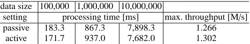
Optimized Configuration for Logical Circuits Table 4 summarizes the performance when F consists of logical gates,
more precisely, when F is a 32-bit comparison, X is Z2, and Y is an extension field GF(28). On Z2, we can apply
the techniques of XOR-free circuits [20]. Shares are shared using a replicated secret sharing scheme [9]. Although the scheme is not generally efficient, it is sufficiently efficient when n=3. Replicated secret sharing supportsZ2, in contrast to
Shamir’s scheme and other general schemes [7, 10]1that are as efficient as Shamir’s secret sharing scheme. Multiplication is shown in Appendix A, and its communication and round costs are the same as GRR-multiplication with k=2 and n=3. WhenX =Z2andY =GF(28), passive execution should be about nine times faster because d = 8. However, the
actual performance is almost the same as that of active execution. This result requires further investigation.
1Although the scheme by Cramer et al. [10] supports an arbitrary ring, the scheme requires a matrix that satisfies the specific condition
Table 4. Performance of Comparison Circuit
data size 100,000 1,000,000 10,000,000
setting processing time [ms] max. throughput [M/s]
passive 183.3 867.3 7,898.3 1.266
active 171.7 937.0 7,682.0 1.302
Comparison with Current High-Performance Passive Implementation For multiplication, shuffling, and comparison,
Sharemind is the fastest implementation, and throughputs are about 0.5, 0.4, and about 0.05 M/s on three-party server machine environments [4, 21]. The throughputs on our implementation were about 6.2, 1.4, and 1.3 M/s on a notebook PC environment. Thus, our active multiplication, shuffling, and comparison were faster than throughputs of passive imple-mentations. Therefore, we claim that our non-robust active construction is sufficiently practical with respect to efficiency.
6
Conclusion
We proposed constructing a non-robust, actively, and unconditionally secure MPC scheme from passively secure schemes while maintaining efficiency.
Our construction is secure in the t<n/2 setting and can use high-level protocols as optional building blocks if the pro-tocols satisfy tamper-simulatability and haveY-distributions. In addition, the communication cost of our construction is comparable to the known smallest cost in the passive case. We implemented our construction and confirmed its efficiency. As a result, our construction is only several times slower than passively secure MPC schemes in theory and is faster than the current fastest passively secure implementation.
References
1. Z. Beerliov´a-Trub´ıniov´a and M. Hirt. Efficient multi-party computation with dispute control. In Halevi and Rabin [14], pages 305–328.
2. Z. Beerliov´a-Trub´ıniov´a and M. Hirt. Perfectly-secure mpc with linear communication complexity. In R. Canetti, editor, TCC, volume 4948 of Lecture Notes in Computer Science, pages 213–230. Springer, 2008.
3. E. Ben-Sasson, S. Fehr, and R. Ostrovsky. Near-linear unconditionally-secure multiparty computation with a dishonest minority. In R. Safavi-Naini and R. Canetti, editors, CRYPTO, volume 7417 of Lecture Notes in Computer Science, pages 663–680. Springer, 2012.
4. D. Bogdanov, M. Niitsoo, T. Toft, and J. Willemson. High-performance secure multi-party computation for data mining applica-tions. Int. J. Inf. Sec., 11(6):403–418, 2012.
5. P. Bogetoft, D. L. Christensen, I. Damgård, M. Geisler, T. P. Jakobsen, M. Krøigaard, J. D. Nielsen, J. B. Nielsen, K. Nielsen, J. Pagter, M. I. Schwartzbach, and T. Toft. Secure multiparty computation goes live. In R. Dingledine and P. Golle, editors,
Financial Cryptography, volume 5628 of Lecture Notes in Computer Science, pages 325–343. Springer, 2009.
6. M. Burkhart, M. Strasser, D. Many, and X. A. Dimitropoulos. Sepia: Privacy-preserving aggregation of multi-domain network events and statistics. In USENIX Security Symposium, pages 223–240. USENIX Association, 2010.
7. R. Cramer and I. Damgård. Secure distributed linear algebra in a constant number of rounds. In Kilian [19], pages 119–136. 8. R. Cramer, I. Damgård, S. Dziembowski, M. Hirt, and T. Rabin. Efficient multiparty computations secure against an adaptive
adversary. In J. Stern, editor, EUROCRYPT, volume 1592 of Lecture Notes in Computer Science, pages 311–326. Springer, 1999. 9. R. Cramer, I. Damgård, and Y. Ishai. Share conversion, pseudorandom secret-sharing and applications to secure computation. In
J. Kilian, editor, TCC, volume 3378 of Lecture Notes in Computer Science, pages 342–362. Springer, 2005.
10. R. Cramer, S. Fehr, Y. Ishai, and E. Kushilevitz. Efficient multi-party computation over rings. In E. Biham, editor, EUROCRYPT, volume 2656 of Lecture Notes in Computer Science, pages 596–613. Springer, 2003.
11. I. Damgård, M. Fitzi, E. Kiltz, J. B. Nielsen, and T. Toft. Unconditionally secure constant-rounds multi-party computation for equality, comparison, bits and exponentiation. In Halevi and Rabin [14], pages 285–304.
12. I. Damgård and J. B. Nielsen. Scalable and unconditionally secure multiparty computation. In A. Menezes, editor, CRYPTO, volume 4622 of Lecture Notes in Computer Science, pages 572–590. Springer, 2007.
13. R. Gennaro, M. O. Rabin, and T. Rabin. Simplified vss and fact-track multiparty computations with applications to threshold cryptography. In B. A. Coan and Y. Afek, editors, PODC, pages 101–111. ACM, 1998.
14. S. Halevi and T. Rabin, editors. Theory of Cryptography, Third Theory of Cryptography Conference, TCC 2006, New York, NY,
USA, March 4-7, 2006, Proceedings, volume 3876 of Lecture Notes in Computer Science. Springer, 2006.
15. K. Hamada, R. Kikuchi, D. Ikarashi, K. Chida, and K. Takahashi. Practically efficient multi-party sorting protocols from compar-ison sort algorithms. In T. Kwon, M.-K. Lee, and D. Kwon, editors, ICISC, volume 7839 of Lecture Notes in Computer Science, pages 202–216. Springer, 2012.
16. M. Hirt and U. M. Maurer. Robustness for free in unconditional multi-party computation. In Kilian [19], pages 101–118. 17. M. Hirt and P. Raykov. On the complexity of broadcast setup. In F. V. Fomin, R. Freivalds, M. Z. Kwiatkowska, and D. Peleg,
editors, ICALP (1), volume 7965 of Lecture Notes in Computer Science, pages 552–563. Springer, 2013.
18. L. Kamm, D. Bogdanov, S. Laur, and J. Vilo. A new way to protect privacy in large-scale genome-wide association studies. In
19. J. Kilian, editor. Advances in Cryptology - CRYPTO 2001, 21st Annual International Cryptology Conference, Santa Barbara,
California, USA, August 19-23, 2001, Proceedings, volume 2139 of Lecture Notes in Computer Science. Springer, 2001.
20. V. Kolesnikov, A.-R. Sadeghi, and T. Schneider. Improved garbled circuit building blocks and applications to auctions and com-puting minima. In J. A. Garay, A. Miyaji, and A. Otsuka, editors, CANS, volume 5888 of Lecture Notes in Computer Science, pages 1–20. Springer, 2009.
21. S. Laur, J. Willemson, and B. Zhang. Round-efficient oblivious database manipulation. In X. Lai, J. Zhou, and H. Li, editors, ISC, volume 7001 of Lecture Notes in Computer Science, pages 262–277. Springer, 2011.
A
Passive Secure Schemes
Here, we describe the tamper-simulatable protocols discussed in the paper. Scheme 6 is GRR-multiplication, Scheme 7 is DN-multiplication (Scheme 8 is a sub-protocol of DN-multiplication), Scheme 9 is RNG in [12], Scheme 10 is pas-sive resharing, and Scheme 11 is a multiplication on (2,3)-replicated secret sharing. These protocols are all the linear-combinatorial protocols discussed in Section 3 (Proofs are omitted.). Thus, they are all tamper-simulatable by Theorem 1.
Scheme 6 [Protocol] GRR-multiplication
Parameter: the threshold k, the number of parties n,
the points x0, . . . ,xn−1∈ F assigned to parties Parties: P0, . . . ,Pn−1
Input: [[ a ]],[[ b ]]∈[[F]], that is, ai,bi∈ F for each party Pi
Output: [[ ab ]]
1: Each party Piwhere i<2k−1 computes (2k−1,n) share⟨c⟩i:=[[ a ]]i[[ b ]]iand shares it so that parties obtain [[⟨c⟩i]]. (⟨·⟩denotes (2k−1,n) shared value.)
2: Parties compute Lagrange interpolation
∑
i<2k−1
αi[[⟨c⟩i]] with proper coefficientsα0,· · ·, α2k−2to reconstruct (2k−1,2k−1)-share
from x0, . . . ,xn−1∈ F.
Scheme 7 [Protocol] DN-multiplication
Parameter: the threshold k, the number of parties n,
the points assigned to parties x0, . . . ,xn−1∈ F, Parties: P0, . . . ,Pn−1
Input: [[ a ]],[[ b ]]∈[[F]], that is, ai,bi∈ F for each party Pi
Output: [[ ab ]]
1: Parties execute Double Random (Scheme 8) and obtain a (k,n) shared value [[ r ]] and a (2k−1,n) shared value⟨r⟩, both plaintexts are r∈ F. (⟨·⟩denotes (2k−1,n) shared value.)
2: Each party Piwhere i<2k−1 computes⟨c⟩i=[[ a ]]i[[ b ]]i+⟨r⟩iand sends it to P0.
3: P0reconstructs the plaintext c from shares⟨c⟩0, . . . ,⟨c⟩2k−2which were received in the previous step.
4: P0distributes c to all other parties.
5: Each party Picomputes c−[[ r ]]iand outputs it.
Scheme 8 [Protocol] Double Random (passive) Parameter: the threshold k, the number of parties n,
the points assigned to parties x0, . . . ,xn−1∈ F and Van der Monde matrix M Parties: P0, . . . ,Pn−1
Input: none
Output: (k,n) random shared values [[ s0]], . . . ,[[ sn−k]] and (2k−1,n) random shared values⟨s0⟩, . . . ,⟨sn−k⟩
1: Each party Pidoes as follows.
2: generates uniformly random value riinF.
3: Pishares riin two manners, (k,n) and (2k−1) Shamir’s secret sharing schemes, and each party Pjobtains shares rk,i,′ jand r2k′,i,j,
respectively.
Scheme 9 [Protocol] Random Number Generation (passive) Parameter: the threshold k, the number of parties n,
the points assigned to parties x0, . . . ,xn−1∈ F and Van der Monde matrix M Parties: P0, . . . ,Pn−1
Input: none
Output: random shared values [[ s0]], . . . ,[[ sn−k]]
1: Each party Pidoes as follows.
2: generates uniformly random value riinF. 3: Pishares riand each party Pjobtains shares r′k,i,j.
4: Piobtains (sk,i,0, . . . ,sk,i,n−k)=M(r′k,i,0, . . . ,rk,i,n′ −k) and outputs them.
Scheme 10 [Protocol] passive resharing
Parameter: the threshold k, the number of parties n Input: [[ a ]]∈[[F ]] for P0, . . . ,Pk−1
Output: [[ a ]] for all parties (the randomness of shares are different from the input)
1: Parties generate a random shared value [[ r ]]. Let Pi’s share be ri. 2: Parties compute [[ a′]] :=[[ a ]]+[[ r ]].
3: Each party Pisends [[ a′]]ito P0.
4: P0reconstructs the plaintext a′from shares [[ a′]]0, . . . ,[[ a′]]k−1which was received in the previous step.
5: P0distributes a′to all other parties.
6: Each party Picomputes a′−[[ r ]]iand outputs it.
Scheme 11 [Protocol] passive multiplication on (2,3)-replicated sharing
Parties: X, Y, Z
Input: [[ a ]],[[ b ]]∈[[X]], i.e., (a0,a1) and (b0,b1) for X, (a1,a2) and (b1,b2) for Y, and (a2,a0) and (b2,b0) for Z where
a=a0+a1+a2and b=b0+b1+b2 Output: [[ ab ]]
1: X, Y, and Z generate rZX, rXY, and rYZ, respectively. 2: X sends rZXto Z, Y sends rXYto X, and Z sends rYZto Y.
3: X sends cXY:=a0b1+a1b0−rZXto Y, Y sends cYZ:=a1b2+a1b2−rXYto Z, and Z sends cZX:=a2b0+a2b0−rYZto X. 4: Let c0, c1, and c2be c0:=a0b0+cZX+rZX, c1:=a1b1+cXY+rXY, and c2:=a2b2+cYZ+rYZ, respectively.
B
Linear-Combinatorial Protocols
We prove Theorem 1, which states all linear-combinatorial protocols are tamper-simulatable.
First, we show an intuition. For simplicity, the MPC protocol has three rounds, and the adversary sends only one element in each round. Let (c1,c2,c3) and (c1′,c′2,c′3) be the legitimate values and possibly tampered values, respectively,
sent by the adversary in the first, second, and third round.
The simulator can compute (c′1,c′2,c′3) since they depend on only the adversary’s knowledge. The simulator can also compute c1 and c2 since they depend on only the inputs, auxiliary inputs, and values sent by the honest parties in the
first round. The last c3 is a bit problematic since the values sent by the honest parties in the second round depend on
c′1. However, the simulator can compute (c′1 −c1), and the honest parties only compute the linear combination whose
coefficientγis public. Therefore, the simulator can computeγ(c′1−c1) then compute (c′3−c3). Consequently, the simulator
can compute the tamper-difference.
Next, we formally define linear-combinatorial protocols.
Definition 4. (linear-combinatorial protocols)
LetRbe a ring, m, µ, ν ∈ Nbe the numbers of inputs, outputs, and rounds, respectively,{[[ aι]]}ι<m be the inputs, and
{[[ bι]]}ι<µbe the outputs.
A Linear-combinatorial protocol consists of two phases, offline and online. In the offline phase, each party Pilocally
computes online inputs{zi,ι}ι<υi ∈ Rυi by an arbitrary function fi({[[ aι]]i}ι<m)7→ {zi,ι}ι<υi, whereυi ∈Nis the number of
each party’s online inputs.
In eachℓ-th round in the online phase, each party Pisendsηℓ,i,jdata{cℓ,i,j,u}u<ηℓ,i,j ∈ Rηℓ,i,jto each other party Pjwhere
ηℓ,i,j∈N. The sent data are linear combinations of offline inputs{zi,ι}ι<υi and all data received{cℓ′,j′,i,u′}ℓ′<ℓ,j′,i,u′<ηℓ′,j′,i by
the (ℓ−1)-th round. Thus, the linear combinations are represented as cℓ,i,j,u=
∑
ι<υi
γℓ,i,j,ιzι+
∑
ℓ′<ℓ
j′,i u′<ηℓ′,j′,i
γ′
ℓ,i,j,u,ℓ′,j′,u′cℓ′,j′,i,u′, where
eachγℓ,i,j,ιandγ′ℓ,i,j,u,ℓ′,j′,u′are public coefficients. Furthermore, the outputs{[[ bι]]i}ι<µof party Piare linear combinations
of{zi,ι}ι<υi and{cℓ,j′,i,u′}ℓ<ν,j′,i,u′<ηℓ′,j′,i.
In the online phase, computations are restricted to linear combinations. However, the offline phase is allowed to perform arbitrary functions including multiplication in GRR-multiplication and DN-multiplication, and generation of all random numbers used in the protocol. In addition, the linear combination is sufficient to realize share and reconstruction schemes of Shamir’s secret sharing and replicated secret sharing.
Finally, we prove the tamper-simulatability of linear-combinatorial protocols.
Theorem 4. (formal version of Theorem 1) Any linear-combinatorial protocol is tamper-simulatable when [[·]] represents
a shared value of an LSSS.
Proof. (Theorem 4)
Let each c′ℓ,i,j,u denote the actual sent data in the active setting, and let cℓ,i,j,u denote imaginary correct data sent in the
passive setting.
First we prove the following lemma by using the induction method onℓ.
Lemma 2. The simulator can compute interim tamper-differencesδℓ,i,j,u=c′ℓ,i,j,u−cℓ,i,j,ufor any roundℓ < ν, any parties
Piand Pj, and any index of data among the data that Pisends to Pjin the protocol.
Proof. (Lemma 2)
(i) Whenℓ=0, no data have been sent yet, and all interim tamper-differences are 0.
(ii) Whenℓ >0, assuming that all differencesδℓ′,i,j,u=c′ℓ′,i,j,u−cℓ′,i,j,usuch thatℓ′< ℓcan be computed by the simulator
for all i, j<n, u< ηℓ′,i,j, we prove that c′ℓ,i,j,u−cℓ,i,j,ucan be computed by the simulator for all i, j<n, u< ηℓ,i,j.
When Piis honest,δℓ,i,j,uis computed as follows.
δℓ,i,j,u=c′ℓ,i,j,u−cℓ,i,j,u =
∑
ι<υi
γℓ,i,j,u,ιzι+
∑
ℓ′<l j′,i u′<ηℓ′,j′,i
γ′
ℓ,i,j,u,l′,j′,u′c′ℓ′,j′,i,u′−
∑
ι<υi
γℓ,i,j,u,ιzι−
∑
ℓ′<ℓ
j′,i u′<ηℓ′,j′,i
γ′
ℓ,i,j,u,ℓ′,j′,u′cℓ′,j′,i,u′
= ∑
ℓ′<ℓ
j′,i u′<ηℓ′,j′,i
γ′
ℓ′,j′,i,u′δℓ′,j′,i,u′
Note that the adversary’s knowledge of such differences does not imply his/her knowledge of plaintexts. Similarly, when
Piis a corrupted party,δℓ,i,j,uis computed as follows.
δℓ,i,j,u=c′ℓ,i,j,u−cℓ,i,j,u =c′ℓ,i,j,u−
∑
ι<υi
γℓ,i,j,u,ιzι+
∑
ℓ′<ℓ
j′,i u′<ηℓ′,j′,i
γ′
Note that both zιand c′ℓ′,j′,i,u′are known by the adversary/simulator since Piis corrupted.
By the induction hypothesis, Lemma 2 has been proven.
□Lemma 2 Similarly, the outputs{[[ bι]]i}ι<µof party Piare linear combinations of{zi,ι}ι<υiand{cℓ,j′,i,u′}ℓ<ν,j′,i,u′<ηℓ′,j′,i, and a recon-struction scheme of LSSS is also a linear combination of shares; therefore, the adversary can compute the differences in the outputs.
□Theorem 4
C
Proof of Lemma 1
Lemma 1. (closure of tamper-simulatability on independent compositions)
Parallel execution of unconditionally secure tamper-simulatable protocols is tamper-simulatable.
Proof. LetΠ0, . . . , Πℓ−1be constitutive protocols andΠ∗be the entire protocol that is a parallel execution ofΠ0, . . . , Πℓ−1,
and aux0, . . . ,auxℓ−1be auxiliary inputs on protocolsΠ0, . . . , Πℓ−1, respectively.
We can construct a simulatorS∗forΠ∗for an adversary with an auxiliary input aux∗as follows. First, we consider a tamper inΠ0. The difference between the solo execution ofΠ0and parallel executions for an adversary is that in parallel
executions, the adversary can tamper withΠ0 with the help of the views ofΠ1, . . . , Πℓ−1executions. However,
tamper-simulatability guarantees that there exists a simulator for any auxiliary input aux0 that can contain the views of other
executions. Therefore, there exists a simulatorS0that computes a tamper-difference even in parallel executions. ForΠ1
. . . ,Πℓ−1there also exists a simulatorS1, . . . ,Sℓ−1for the same reason.
Consequently, the outputs ofS∗are the sum of the tamper-differences computed byS0, . . . ,Sℓ−1.
□(Lemma 1)
D
Example of Mandatory Building Blocks
The RNG, scalar multiplication/product-sum, addition/subtraction, multiplication, and reveal are all realized on [[F]]dby operations on [[F]]. Note thatFdis trivially homeomorphic toE(F)das a group.
1. RNG : [[ r ]]←([[ r0]],· · ·,[[ rd−1]]), where each [[ ri]] is generated by an RNG on [[F]], and is also random on [[F]]d
as [[E(F)d]].
2. scalar multiplication : [[ ar ]]←([[ ar0]],· · ·,[[ ard−1]]), where [[ a ]]∈[[F]] and [[ r ]]∈[[F]]d.
3. scalar product-sum : [[∑
i<m
airi]]←([[
∑
i<m
ai(ri)0]],· · ·,[[
∑
i<m
ai(ri)d−1]]), where m∈Nand for each i<m, [[ ai]]∈[[F]]
and [[ ri]]∈[[F ]]d.
4. addition/subtraction : [[ r+s ]]←([[ r0]]+[[ s0]],· · ·,[[ rd−1]]+[[ sd−1]]), where [[ r ]],[[ s ]]∈[[F]]d.
5. multiplication : [[ rs ]]←([[ ∑
i,j<d
αi,j,0risj]],· · ·,[[
∑
i,j<d
αi,j,d−1risj]]) with a sequence of coefficient matricesα0,· · ·, αd−1∈
Fd2
determined by an irreducible polynomial ofE(F)d. For example, when d=2 and the irreducible polynomial is
X2+X+1,α0=
( 1 0 0−1
) ,α1=
( 0 1 1−1
) . 6. (correct) reveal: shown in Scheme 12.
If addition/subtraction and multiplication are both tamper-simulatable, the above mandatory building blocks are also tamper-simulatable since they will be (except for reveal) parallel executions of addition/subtraction and multiplication. Reveal in Scheme 12 is correct by itself.
In LSSS, arbitrary quadratic functions, including product-sum functions, are computed with the same communication and round cost as multiplication in the passive setting. Thus, the communication and round cost of scalar multiplication/ product-sum and multiplication onE(F)dare the same as d parallel multiplications onF or 1 multiplication on nativeE(F)d.
E
Examples of Optional Building Blocks
Linear transformations including addition/subtraction, and quadratic functions including multiplication are already shown as mandatory building blocks in Appendix D; They can be used as optional building blocks.
Resharing used in reshare-based shuffling [21] can also be used as an optional building block. In this shuffling, input shared values a0, . . . ,am−1are randomly permuted by k parties with random permutation dataπdistributed (as plaintexts)