(will be inserted by the editor)
On metric regularity of Reed-Muller codes
Alexey Oblaukhov
Received: date / Accepted: date
Abstract In this work we study metric properties of the well-known family of binary Reed-Muller codes. Let A be an arbitrary subset of the Boolean cube, and Ab be the metric complement of A — the set of all vectors of the Boolean
cube at the maximal possible distance from A. If the metric complement of Ab
coincides with A, then the set A is called a metrically regular set. The problem of investigating metrically regular sets appeared when studying bent functions, which have important applications in cryptography and coding theory and are also one of the earliest examples of a metrically regular set. In this work we describe metric complements and establish the metric regularity of the codes RM(0, m) and RM(k, m) for k > m−3. Additionally, the metric regularity of the codes
RM(1,5) and RM(2,6) is proved. Combined with previous results by Tokareva N. (2012) concerning duality of affine and bent functions, this establishes the metric regularity of most Reed-Muller codes with known covering radius. It is conjectured that all Reed-Muller codes are metrically regular.
Keywords metrically regular set· metric complement·covering radius· bent function·Reed-Muller code·deep hole
A. Oblaukhov
Sobolev Institute of Mathematics, Novosibirsk, Russia
E-mail: [email protected]
1 Introduction
The problem of investigating and classifyingmetrically regular sets was posed by Tokareva [17, 18] when studying metric properties ofbent functions[13]. A Boolean function f in even number of variablesm is called abent function if it is at the maximal possible distance from the set of affine functions.
Bent functions have various applications in cryptography, coding theory and combinatorics [7, 18]. In cryptography, bent functions are valued because of their outstanding nonlinearity, which allows one to construct S-boxes for block ciphers which possess high resistance to the linear cryptanalysis [7]. However, many prob-lems related to bent functions remain unsolved; in particular, the gap between the best known lower and upper bound on the number of bent functions is ex-tremely large; currently known constructions of bent functions are rather scarse. In 2010 [16], Tokareva has proved that, like bent functions are maximally distant from affine functions, affine functions are at the maximal possible distance from bent functions, thus establishing themetric regularityof both sets. This discovery arouses interest in studying the property of metric regularity in order to better understand the structure of the set of bent functions.
From the coding theory standpoint, bent functions form the set of points at the maximal possible distance from the Reed-Muller code of the first order in an even number of variables. Therefore, the aforementioned result by Tokareva establishes the metric regularity of the codesRM(1, m) for even m. Reed-Muller codes are extensively studied for many years, but their metric properties, like the covering radius, are very elusive and are being discovered to this day; just recently, Wang has found the covering radius of the codeRM(2,7) to be equal to 40 [19]. These problems put Reed-Muller codes in our focus of the research of metric regularity. Let us briefly overview the results obtained in this area. As mentioned be-fore, Tokareva [16] has established the metric regularity of the sets of affine/bent functions. Metric regularity of several classes of partition set functionsis studied in [15], while the works [4, 5] touch upon metric properties of certain subclasses of bent functions. Metric regularity has been actively investigated by the author: metric complements of linear subspaces of the Boolean cube are studied in the paper [10], while the works [11] and [12] are studying possible sizes of the largest and smallest metrically regular set.
In this work we investigate the metric regularity of Reed-Muller codes. Nat-urally, the knowledge of the covering radius of the code is necessary for working with the set of its most distant points. Among the codes of high order, covering radii of the codes RM(k, m) for k > m−3 are known. The covering radius of
RM(1, m) for oddm >7 is unknown, but has been determined forRM(1,5) [1] andRM(1,7) [8, 3]. In [14], Schatz has found the covering radius of RM(2,6), while recently Wang has established the covering radius of RM(2,7) [19]. For
m >7, the covering radius ofRM(2, m) is currently unknown. We prove that the codesRM(k, m), for k= 0 and k >m−3 and the codesRM(1,5),RM(2,6) are metrically regular and also describe their metric complements in most cases.
from vectors to the puncturedRM(m−3, m) code, based on the “Covering codes” [2] book by Cohen et al. Following the book, we calculate the covering radius of the Reed-Muller code of orderm−3, and utilizing the method further, we obtain the metric complement of this code. The description of the complement allows us to establish that only the functions from RM(m− 3, m) are contained in the second metric complement, which proves the metric regularity of the Reed-Muller codes of orderm−3. We then proceed to establish the metric regularity of the codeRM(2,6), based on the results obtained for the codesRM(2,5) and
RM(1,5), since the former can be constructed from the latter using the (u,u+v) construction. The paper concludes with an overview of the results obtained and a hypothesis concerning the metric regularity of all Reed-Muller codes.
2 Definitions and examples
LetFn2 be the space of binary vectors of lengthnwith the Hamming metric. The Hamming distanced(·,·) between two binary vectors is defined as the number of coordinates in which these vectors differ, whilewt(·) denotes theweightof a vector, i.e. the number of nonzero values it contains. The plus sign + denotes addition modulo two (componentwise in case of vectors), while the componentwise product of two binary vectors is denoted by∗.
LetX⊆Fn
2be an arbitrary set andy∈Fn2 be an arbitrary vector. The distance from the vectory to the setX is defined as
d(y, X) = min x∈Xd(y, x).
Thecovering radiusof the setX is defined as
ρ(X) = max z∈Fn2
d(z, X).
The setX withρ(X) =ris also called acovering code[2] of radiusr. Consider the set
Y ={y∈Fn2|d(y, X) =ρ(X)}
of all vectors at the maximal possible distance from the set X. This set is called the metric complement [10] of X and is denoted by Xb. Vectors from the metric
complement are sometimes called thedeep holesof a code. If b b
X=Xthen the set
X is said to bemetrically regular [18].
Note that metrically regular sets always come in pairs, i.e. if Ais a metrically regular set, then its metric complement Ab is also a metrically regular set and
both of them have the same covering radius. For some simple examples of metric complements and metrically regular sets, refer to [10–12].
The following trivial auxiliary lemma, established in [10], will be used through-out the paper.
Lemma. LetC ⊆Fn
2 be a linear code. Then ρ(Cb) =ρ(C)and a vectorx∈Fn2 is
in b b
Let Fm be the set of all Boolean functions in m variables. The Reed-Muller code of orderkinmvariables is defined as:
RM(k, m) ={f∈ Fm: deg(f)6k},
where deg(·) denotes the degree of thealgebraic normal form (ANF)of a function. The Reed-Muller code can be also represented as the set of value vectors of the corresponding functions. Throughout the paper we will often switch between these two representations, sometimes “on the fly”. In most cases, m will denote the number of variables, whilen:= 2mwill denote the dimension of the space of value vectors, which have coordinates numbered from 0 to 2m−1. Thei-th coordinate of a value vector is the value of the corresponding function at the binary vector of lengthmwhich is the binary representation of the numberi. Weights of functions, distances between functions and between a function and a set of functions are defined as distances between their value vectors.
Throughout the paper, vectors of length mand square m×mmatrices will be denoted using roman typestyle letters (e.g., x,A), while vectors of length n
and vectors derived from them, as well as matrices related to such vectors, will be denoted using bold letters (e.g.,v,B).
Let f andg be two functions in m variables. Let LAb : Fm2 →Fm2 denote the affine transformation of the variables with the matrix A and the vector b:
(f◦LbA)(x) =f(Ax + b).
Here◦ denotes the operation of composition of two functions. If the vector b is zero, it will be omitted from the notation. Functions f andg are called linearly equivalentif one can be obtained from the other by applying a nonsingular linear transformation to the variables, i.e.f =g◦LA, where det A6= 0.
Extended affine equivalence is more common when classifying Boolean func-tions: functions f and g are called EA-equivalent if there exists a nonsingular binary matrix A, a Boolean vector b of length m and a functionh of degree at most 1 such thatf =g◦LbA+h.
For our study we will use a variant of these two equivalence relations, which will be referred to asextended linear equivalence (to the power ofk). Functionsf
andgare called ELk-equivalentif there exists a nonsingular binary matrix A and a functionh of degree at mostksuch that
f=g◦LA+h.
It is easy to see that this relation is indeed an equivalence. If two functionsf and
g are ELk-equivalent, we will denote it by f ∼k g. We will also write f =k g iff
and g differ by a function of degree at most k. Note that the last relation is a subrelation of the ELk-equivalence.
No Representativef Addedg∈Rb1,5 C(g) Sumh=f+g C(h)
0 0 — — — —
1 2345 123+14+25 22 2345+123+14+25 12
2 2345+14 123+14+25 22 2345+123+25∼2345+123+34 8
3 2345+24 2345+123+24+35 14 123+35∼123+14 21
4 2345+24+35 2345+123+24+35 14 123 19
5 2345+14+25 123+14+25 22 2345+123 6
6 2345+123 123+14+25 22 2345+14+25 5
7 2345+123+12 12+34 28 2345+123+34 8
8 2345+123+34 12+34 28 2345+123+12 7
9 2345+123+14 14+25 28 2345+123+25∼2345+123+34 8
10 2345+123+45 12+45 28 2345+123+12 7
11 2345+123+12+34 12+34 28 2345+123 6
12 2345+123+14+25 123+14+25 22 2345 1
13 2345+123+12+45 12+45 28 2345+123 6
141 2345+123+24+35 2345+123+24+35 14 0 0
15 2345+123+145 123+14+25 22 2345+145+14+25∼2345+123+12+34 11
16 2345+123+145+45 123+145+45+24+35 26 2345+24+35 4
17 2345+123+145+24+45 2345+123+24+35 14 145+35+45∼123+14 21
18 2345+123+145+24+35 2345+123+24+35 14 145∼123 19
19 123 2345+123+24+35 14 2345+24+35 4
20 123+45 2345+123+24+35 14 2345+24+35+45∼2345+24+35 4
21 123+14 123+14+25 22 25∼12 27
222 123+14+25 123+14+25 22 0 0
23 123+145 123+14+25 22 145+14+25∼145+25∼123+14 21
24 123+145+23 23+45 28 123+145+45∼123+145+23 24
25 123+145+24 123+15+24 22 145+15∼123 19
263 123+145+45+24+35 123+145+45+24+35 26 0 0
27 12 12+34 28 34∼12 27
284 12+34 12+34 28 0 0
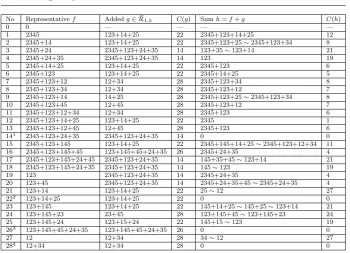
Table 1 Table of even weight coset classes ofR1,5. Classes marked with a superscript are
the classes which constitute Rb1,5.C(·) denotes the No of the class the function belongs to.
Functions in the table are presented in an abbreviated notation: the numberi1i2. . . ikstands
for the monomialxi1xi2. . . xik. For example, the representative function for the class 14 is x2x3x4x5+x1x2x3+x2x4+x3x5.
3 The Reed-Muller codeR1,5
Let us first consider a special case — the code R1,5. This is the set of affine functions, but in the odd number of variables, so it is not covered by the result of Tokareva concerning bent functions.
In 1972, Berlekamp and Welch presented a partition of all cosets of the code
R1,5 into 48 classes with respect to the EA-equivalence and obtained weight dis-tributions for each class of cosets [1]. The largest minimal weight (and therefore the covering radius of the code) among all classes is equal to 12, and is attained on four coset classes (classes 14, 22, 26 and 28 in Table 1). These four classes constitute the metric complement ofR1,5.
Theorem 1 The codeR1,5 is metrically regular.
Proof. SinceR1,5 is linear, it follows that ρ(Rb1,5) =ρ(R1,5) = 12 andf ∈Rbb1,5 if and only iff+Rb1,5=Rb1,5. Thus, in order to establish the metric regularity of
R1,5, we have to prove that for everyf /∈ R1,5it holdsf+Rb1,56=Rb1,5.
of the class representatives were modified from their original variants using simple variable swaps (for the original representatives the reader is referred to Table 5 in the appendix of the paper).
Let us show that only the R1,5 code itself is contained in the second metric complement. Let fc ∈ R/ 1,5 be a function from a certain coset equivalence class
C, and assume that the function fc+gc, where gc ∈ Rb1,5, does not belong to any of the 4 equivalence classes from the complement Rb1,5. This implies that
fc+Rb1,56=Rb1,5 and thusfcis not in the second metric complement.
Let now f /∈ R1,5 be an arbitrary function from the classC, and let (A,b, h) be the matrix, the vector and the affine function such that
f◦LbA+h=fc.
Denote
gf = (gc+h)◦(LbA)
−1
.
Then the functionf+gfis EA-equivalent tofc+gcand therefore does not belong toRb1,5. Since (LbA)
−1=LA−1b
A−1 ,gf belongs toRb1,5and thereforef+Rb1,56=Rb1,5, which means thatf /∈ b
b R1,5.
Thus, if we prove that f+g /∈Rb1,5 for somef ∈C and someg ∈Rb1,5, we will prove that no function from the equivalence class C is in the second metric complement.
The proof can be found in Table 1: for a representative f from each even weight coset class we find a function g ∈ Rb1,5 such that f +g is equivalent to the representative of some class which is not inRb1,5. Thus, the second metric
complement b b
R1,5contains only the codeR1,5itself, proving thatR1,5is metrically regular.
u t
Almost all equivalences presented in the fifth column of Table 1 are variable swaps or simple additions of the formxi→xi+ 1,xi →xi+xj or (for the class 20)xi →xi+xj+xk for certaini, j, k.
4 The Reed-Muller codes of orders 0,m,m−1 andm−2
The Reed-Muller codes of orders 0,mandm−1 coincide with the repetition code, the whole space and the even weight code respectively. It is trivial that all of them are metrically regular.
The covering radius of the Reed-Muller code of order m−2 is equal to 2 [2]. By definition, this code consists of all Boolean functions of degree at mostm−2. Since functions of degree mhave odd weights, while functions of smaller degree have even weights, functions of degree m are at distance 1 from Rm−2, while functions of degreem−1 are at distance 2 and therefore
b
Rm−2=Rm−1\ Rm−2.
Since Rm−2 is linear, ρ(Rbm−2) = ρ(Rm−2) = 2 and thus functions of degree
5 The Reed-Muller codes of orderm−3: Syndrome matrices
McLoughlin [6] has proved that
ρ(Rm−3) =
(
m+ 1, ifmis odd,
m+ 2, ifmis even.
We are going to reestablish this result following the book “Covering codes” by Co-hen et al., since our new results that follow rely on the methods and terminology described in the book. In particular, we will describe the method of obtaining the covering radius ofRm−3 using syndrome matrices as it is presented in the book, with few minor adjustments. After that we will proceed to study the metric com-plement ofRm−3. Results in Section 5 and 6, as well as general results concerning the covering radius ofRm−3, belong to Cohen et al. [2], while all subsequent re-sults concerning the metric complement and the metric regularity of the code have been obtained by the author.
Let us first consider the covering radius of the punctured Reed-Muller code
R◦m−3, i.e., the code without the 0-th coordinate (which corresponds to the value of the function at zero). LetH denote the parity check matrix of this code. The matrixHcoincides with the parity check matrix of the non-punctured codeRm−3, but with the first all-one row and the first column removed. Since Rm−3 is dual to the codeR2, the rows ofHare punctured value vectors of the functions
x1, . . . , xm, x1x2, x1x3, . . . , xm−1xm.
The syndromesof an arbitrary vectorv∈Fn−1
2 is the productHv
T. Let us
consider the syndrome s as an m×m symmetric matrix S, where the element
si,j of the matrix is equal to the component of the syndrome corresponding to the row xixj of the parity check matrix H, while the diagonal element si,i is equal to the component of the syndrome corresponding to the rowxi of the matrixH. Thus we have built a one-to-one correspondence between all cosets ofR◦m−3 and all symmetric binary matrices (“syndrome matrices”).
Lete◦1, . . .e ◦ m∈Fn
−1
2 be the punctured value vectors of the functionsx1, . . . , xm. Notice that the row ofHcorresponding to the functionxixjis the componentwise producte◦i ∗e◦j.
Consider anm×(n−1) matrixBv which hase◦i ∗vas itsi-th row. Then the
symmetric matrix Sv = BvBTv corresponds to the syndrome HvT of the vector v. It is easy to see that iff is a function with a punctured value vector equal tov, then the set of nonzero columns of Bv is precisely the support of the function f
(bar, possibly, the all-zero vector). The number of nonzero columns inBv is equal to the weight of the vectorv.
Given an arbitrary vectorv∈Fn2−1, its distance from the code is equal to the weight of the coset leader:
d(v,R◦m−3) = min
u:HuT=HvTwt(u).
Using the established correspondences between syndromes and symmetric matri-ces, we can rewrite this as follows:
d(v,R◦m−3) = min
u:BuBTu=Sv
whereCol(Bu) is the number of nonzero columns in the matrixBu. Let us denote the minimum on the right byt(S) := min
u:BuBTu=S
Col(Bu).Then
d(v,R◦m−3) =t(Sv),
and, since the correspondence between all syndromes and all symmetric matrices is one-to-one, we have
ρ(R◦m−3) = max
v d(v,R ◦
m−3) = max
S t(S).
Moreover, a vector v is in the metric complement Rb◦m−3 if and only if t(Sv) =
ρ(R◦m−3).
Let us call any matrix B such that BBT = S a factor of S. We can thus describe the valuet(S) asthe minimum number of nonzero columns in a factor over all factors of S of the form Bu, where u ∈ Fn2−1. We will call any factor achieving this minimum aminimal factor.
Let us now expand the definition of the valuet(S).
Lemma 1 Let Sbe a symmetric matrix, and letBbe its factor (i.e.BBT=S). The following operations do not change the property ofBbeing a factor ofS:
1. deleting a zero column; 2. deleting two equal columns; 3. swapping any two columns;
4. adding an arbitrary vectorbto each column from some subset of columns ofB
of even size, given that all columns of this subset sum to zero.
Proof. The proof is routine and is left to the reader. ut
Since the subsets of nonzero columns of matrices{Bu:u∈Fn−1
2 }are precisely all possible subsets of nonzero columns of lengthm, Lemma 1 allows us to remove zero columns from allowed factors and ignore the possibility of duplicate columns and thus reformulate the definition of the value t(S) in the following manner, allowing the use of arbitrarily-sized matrices:
The valuet(S)is equal to the minimum number of columns in a factor over all factors ofS. Any factor achieving this minimum is called a minimal factor ofS.
Moreover, any factor B of S corresponds to exactly one factor of the initial formBu— the factor with the set of nonzero columns coinciding with the set of nonzero columns of B. Therefore, presenting any minimal factor for a symmetric matrixSallows us to obtain a coset leader ufor the coset which this symmetric matrix represents.
6 The Reed-Muller codes of orderm−3: Covering radius
In order to determine the covering radius of R◦m−3 we will now investigate the maximum possible value oft(S). Obviously,
t(S)> min
for any matrixS, and therefore max
S t(S)>m.
This gives us a trivial lower bound. The following proposition provides a simple upper bound:
Lemma 2 Let S be a symmetric matrix, and let Bbe its minimal factor. Then all proper subsets of columns of Bare linearly independent.
Proof. See [2], pp. 249–250.
u t
Corollary 1 t(S)6m+ 1for any symmetricm×mmatrixS.
Proof. Assume that for some symmetric matrix S it holds t(S) > m+ 2. This means that any minimal factorB ofShas at leastm+ 2 columns and therefore contains a linearly dependent proper subset of columns, which contradicts Lemma
2. ut
This bound, combined with the previous one, shows us that the largest value oft(S) is eithermorm+ 1. The following result describes the matrices with the larger value oft(S).
Lemma 3 Let S be a symmetric matrix. Then t(S) = m+ 1 if and only if
rank(S) =mandS has an all-zero diagonal. Proof. ⇐=
Assume that the matrixSis nonsingular and has an all-zero diagonal, and let
Bbe any of its factors. Notice that the vector consisting of all diagonal entries of the matrix Sis the sum of all columns of B. Therefore all columns of Bsum to zero, which means that all its nonzero columns form a linearly dependent set of vectors. Since rank(B)>rank(S) =m, the matrix Bhas at leastm+ 1 nonzero columns and thereforet(S) =m+ 1.
=⇒
Assume thatt(S) =m+1. LetBbe a minimal factor ofS. Note that all proper subsets of columns ofBare linearly independent by Lemma 2, which implies that all columns ofBsum to zero, sinceBis anm×(m+ 1) matrix. Since the vector consisting of diagonal elements of S is the sum of all columns of B, S has an all-zero diagonal.
Assume that rank(S)< m. Then there exists a subset of rows inS summing to0; we denote these rows bySi1,Si2, . . . ,Sip. SinceSi=BiB
T, this implies
(Bi1+. . .+Bip)B
T
=0.
Denoteb=Bi1+. . .+Bip. From the above it follows that the sum of certain
columns ofB(those corresponding to the 1’s in the vectorb) is equal to zero. If the vectorbis zero, then rank(B)< mand it must have a linearly dependent proper subset of columns, contradiction with Lemma 2.
If it is nonzero and not an all-ones vector, then we obtain a proper subset of columns ofBwhich sum to 0, contradiction with Lemma 2.
Ifmis even, then the number of columns inBis odd and thereforebbT= 1, which contradictsbBT=0.
If m is odd, then the number of columns in B is even and all rows have an even number of ones, and, by Lemma 1, we can add any column ofB to all its columns and then remove a zero column from the resulting matrix, keeping it a factor ofS, which contradicts the minimality ofB.
Thus, rank(S) is equal tom.
u t
Note that a matrixSwith the properties described in the lemma (nonsingular with an all-zero diagonal) exists if and only ifmis even (see e.g. [2], p. 249). This means that
max
S t(S) =m+ 1−π(m),
whereπ(m) is the parity function, equal to 1 for oddmand to 0 for evenm.
7 The Reed-Muller codes of orderm−3:m is even
7.1The covering radius and the metric complement of the punctured code
Let the number of variablesmbe even. From previous sections we have:
ρ(R◦m−3) = max
S t(S) =m+ 1.
A vector v∈Fn−1
2 is in the metric complement of R
◦
m−3 if and only if t(Sv) =
m+ 1. The following statements will help us to characterize the syndromes of such vectors:
Lemma 4 Let S be a symmetric m×m matrix, meven. Then t(S) =m+ 1 if and only ifS has a factor of rankmwithm+ 1columns which sum to zero. Proof. =⇒
Assume thatt(S) =m+ 1 and letBbe an arbitrary minimal factor ofS. By Proposition 1, rank(S) =mandShas an all-zero diagonal. Therefore, rank(B) =
mand all its columns sum to zero.
⇐=
Let Bbe a factor ofSof rankmwithm+ 1 columns which sum to0. Assume thatt(S) =k6mand letDbe an arbitrary minimal factor ofSwith
kcolumns. Since the sum of all columns of a factor is the vector consisting of the diagonal elements of S, the sum of all columns of D is also equal to zero. This implies that rank(D)< m, and therefore rank(S)< m.
It is easy to see that each proper subset of columns ofBis linearly independent. Notice that the existence of a factor with this property is shown to contradict with the assumption “rank(S)< m” in the proof of Proposition 1, and in the case when
mis even the proof does not rely on the minimality ofB. Thus,t(S) =m+ 1 andBis a minimal factor ofS.
It is easy to see that Lemma 4 describes all minimal factors of all matricesS
satisfyingt(S) =m+ 1. Let us construct the following set:
U ={u∈Fn2−1:Buhasm+ 1 nonzero columns,mof which are
linearly independent and all of them sum to zero}.
Trivially, the set of matrices {Bu : u ∈ U} (up to columns permutations and zero columns removal) includes exactly all minimal factors described in Lemma 4. Therefore, ift(S) =m+ 1 for some matrix S, then there exists a vector u∈ U such thatS=BuBTu. Conversely, for anyu∈U it holdst(BuBTu) =m+ 1. Thus,
the vectors from the set U cover all cosets contained in the metric complement of
R◦m−3:
b R◦m−3=
[
u∈U
u+R◦m−3
.
7.2The covering radius and the metric complement of the non-punctured code
We have obtained the covering radius and described the metric complement of the punctured code. Let us return to the regular, non-punctured Reed-Muller code
Rm−3. Since it is obtained from the punctured code by adding a parity check bit at the 0-th coordinate, the following result will be of use:
Lemma 5 LetC be a code with the covering radiusrand the metric complement
b
C. LetCπbe the code obtained fromC by adding a parity check bit to all codewords ofC (in the front). Thenρ(Cπ) =r+ 1and Cbπ is obtained fromCb by
1. adding a parity check bit to all vectors in case if ris odd or
2. adding an inversed parity check bit to all vectors in case if ris even.
Proof. Obviously,ρ(Cπ)6r+ 1.
Let us prove (2). Assume thatris even. Denote
Ci={c∈C:wt(c) mod 2 =i}, Cbi={c∈Cb:wt(c) mod 2 =i}, i= 0,1.
Sinceris even, vectors fromCb0are at distancerfromC0and at a larger distance from C1. Similarly, vectors from Cb1 are at distance r from C1 and at a larger distance fromC0.
Let c0= (, c), wherec /∈Cband∈ {0,1}. Thend(c0, Cπ)6d(c, C) + 16r. Letc∈Cb1. Thend((1, c), Cπ) = min(d(c, C1), d(c, C0)+1) =r, whiled((0, c), Cπ) = min(d(c, C1) + 1, d(c, C0))> r.
Let c ∈ Cb0. Similarly, d((1, c), Cπ) = min(d(c, C1), d(c, C0) + 1) > r, while
d((0, c), Cπ) = min(d(c, C1) + 1, d(c, C0)) =r.
Therefore, vectors {(1, c)|c ∈ Cb0} ∪ {(0, c)|c ∈ Cb1} are the only ones at a distance larger thanrfromCπ, and this distance can be only equal tor+ 1. The claim (2) of the lemma is proved.
The proof of the case (1) is completely similar to the above, but with some sets switched around.
Using this lemma we find that the covering radius of the non-punctured Reed-Muller codeRm−3is equal tom+ 2 and its metric complement can be described as follows:
b Rm−3=
[
u∈U
((π(u),u) +Rm−3).
Let fv denote the function with the value vector v ∈ Fn2 (non-punctured). Recall that the set of nonzero columns of the matrixBv◦coincides with the support
of the functionfv, bar, possibly, the zero vector. Since all vectors in U have odd weights and added parity check bit corresponds to the value of the function at the all-zero vector, we can describe the metric complement ofRm−3 in terms of functions instead of their value vectors as follows:
b Rm−3=
[
g∈G
(g+Rm−3),
where
G={f(1,u):u∈U}={g: supp(g) ={0,x1,x2. . . ,xm,x1+. . .+ xm},
{x1, . . . ,xm}are linearly independent}.
All functions inG form an equivalence class with respect to the linear equiv-alence. Recall that two functionsf andg are called ELk-equivalentif there exists a nonsingular binary matrix A and a function h of degree at mostk such that
g=f◦LA+h. It is now easy to see that a functiong is inRbm−3 if and only if it is ELm−3-equivalent to some function fromG. Since all functions in the metric complement are equivalent, we can pick any function from it as the reference for equivalence (and we will change this reference when it is convenient). We will call the ELm−3-equivalence just “equivalence” for brevity from now on.
Let us give an explicit (algebraic normal form) description of a certain function fromG. Denote byg∗ the function with the support {0,e1,e2, . . . ,em,1}, where ei ∈Fm2 is the vector with 1 only in thei-th coordinate. Clearly, g
∗ ∈
G and it is straightforward to construct the algebraic normal form of this function: it is the sum of all monomials containing an even number of variables, excluding the monomial with all variables included:
g∗(x) = 1 +
m
2−1
X
k=1
X
16i1<...<i2k6m
xi1xi2. . . xi2k.
This function is equivalent to the sum of all monomials containingm−2 variables, so let us use this last function asg∗ moving forward. Let xi denote the product of all m variables exceptxi, and letxixj denote the product of all m variables except xi andxj. Using these conventions, we can write this new representative function as follows:
g∗(x) := X 16i<j6m
7.3Metric regularity
We have established that
b
Rm−3={g:g m−3
∼ g0},
where g0 is an arbitrary function from the class G (or from Rbm−3), and have constructed a certain representative of this equivalence class —g∗.
Since the codeRm−3is linear,ρ(Rbm−3) =ρ(Rm−3) =m+ 2 and a functionf is in b
b
Rm−3if and only iff+Rbm−3=Rbm−3. Let us prove the metric regularity of
Rm−3by proving that no functions other that those contained inRm−3 preserve the metric complement under addition.
Letf /∈ Rm−3be an arbitrary function. SinceRbm−3is an ELm−3-equivalence class, in order to show thatf+Rbm−36=Rbm−3 it is enough to show there exists a functionf0such thatf0m∼−3f andf0+Rbm−36=Rbm−3.
Case 1. Let f /∈ Rm−3 be a function of degree greater than m−2. Since ELm−3-equivalence preserves the degree for functions of degree higher than m−
3, any g ∈ Rbm−3 has degree m−2 (like g∗), while f +g has a higher degree and therefore cannot be equivalent to any of the functions from Rbm−3. Thus, functions of degree greater than m−2 do not preserve any function from the
metric complement and therefore cannot be in b b Rm−3.
Case 2.Letf /∈ Rm−3be a function of degreem−2. We can uniquely present it as follows:
f(x) = X (i,j)∈I
xixj+h(x),
where deg(h)< m−2. Denote by ˜f the following quadratic function:
˜
f(x) := X (i,j)∈I
xixj.
We will call ˜f thequadratic dual off.
The following result would be of use when handling this case:
Lemma 6 Let f and g be two functions of degree m−2. Then f m∼−3 g if and only if their quadratic duals are EL1-equivalent (EA-equivalent).
Proof. Since ELm−3-equivalence allows us to add functions of degree up tom−3, we will assume that both f and g contain only monomials of degree m−2. In what follows we will discard monomials of degree less than m−2 when talking about ELm−3-equivalence, and we will discard monomials of degree less than 2 when talking about EL1-equivalence.
Let f(x) = P
(i,j)∈I
xixj be the ANF of f. Let us perform the following simple
nonsingular linear transformation of variablesLij:
Lij:
(
xi←xi+xj,
The function f changes under this transformation (disregarding monomials of degree less thanm−2) in the following manner:
Lij:
xixk←xixk ∀k6=i,
xjxk←xjxk+xixk ∀k6=i, j,
xkxl←xkxl ∀k, l6=i, j.
Let f1denote the function obtained after this transformation. Then it is easy to see that the dual function ˜f1is obtained from the dual function ˜f (disregarding monomials of degree less than 2 since we consider EL1-equivalence) by the following linear transformation:
Lji:
(
xj ←xj+xi,
xk←xk ∀k6=j.
which is simply the transposed transformation.
Assume now that g is obtained from f using some linear transformation L. Trivially,Lcan be decomposed into a sequence of simple transformations:
L=Li1j1◦Li2j2◦. . .◦Lisjs.
From the above we can see that the dual function ˜g is obtained from ˜f using the following transformation ˜L:
˜
L=Lj1i1◦Lj2i2◦. . .◦Ljsis
which is a sequence of transposed simple transformations.
Thus we have established that, if f m∼−3 g, then ˜f ∼1 ˜g. The reverse can be shown using similar argumentation.
u t
It is known that any quadratic Boolean function is EA-equivalent to the func-tion of the form x1x2 +x3x4+. . .+x2k−1x2k for some k 6 m2, and any two functions of this form with different number of variables are not EA-equivalent one to the other. Using this result and Lemma 6 we conclude thatf is equivalent to the functionpk for somek(0< k6 m2), where
pk(x) =x1x2+x3x4+. . .+x2k−1x2k= k
X
i=1
x2i−1x2i.
Trivially,g∗ is equivalent to pm
2. Then pk+p
m
2 is equivalent to p
m
2−k, which is (by Lemma 6) not equivalent to pm
2 and therefore not equivalent to g
∗
. This
means thatf+Rbm−36=Rbm−3and thereforef /∈Rbbm−3.
Since all functions which are not inRm−3have degreem−2 or higher, we have just shown that none of them are in the second metric complement, and therefore
8 The Reed-Muller codes of orderm−3:m is odd
8.1The covering radius and the metric complement of the punctured code
Let the number of variables m be odd. Many arguments for this case are simi-lar or identical to the ones for the previous case, however, the proof a bit more complicated. From Section 6 we have:
ρ(R◦m−3) = max
S t(S) =m,
and a vector v is in the metric complement of R◦m−3 if and only if t(Sv) = m. The following lemma will help to characterize matrices achieving this maximum:
Lemma 7 Let Sbe a symmetricm×mmatrix, wheremis odd. Thent(S) =m
if and only ifShas anm×mfactor which is either nonsingular, or has rankm−1
and all columns summing to zero.
Proof. =⇒
Assume that t(S) =m and let Bbe a minimal factor of S with m columns. If the rank of B is smaller than m−1, then Bhas a proper subset of columns summing to zero, contradicting the minimality ofB, so the rank of the factor must be at leastm−1. If the rank ism, the proof is finished.
Assume that rank(B) =m−1. Then some subset of columns ofBmust sum to zero. SinceBis minimal, it cannot be a proper subset by Lemma 2, therefore all columns ofBmust sum to zero.
⇐=
Clearly, t(S)>rank(S), so if S= BBTfor some nonsingular m×mmatrix
B, then the proof is finished.
Let S=BBTfor someBof rankm−1 with all columns summing to zero. Assume thatt(S) =k6m−1 and letDbe a minimal factor of S. Since the sum of all columns of any factor is the vector composed of the diagonal elements ofS, the sum of all columns ofDis also zero.
Assume that k= m−1. Then Dhas an even number of columns, and each row has an even number of ones, so we can add an arbitrary vector to all columns ofDwhile keeping it a factor ofSusing Lemma 1. Let us add the first column of
Dto all its columns. Now the first column ofDis zero and we can remove it by Lemma 1. We have now obtained a factor of S with fewer columns thanDhas, which contradicts the minimality ofD.
Therefore,kcan be at mostm−2. Since all its columns sum to zero,Dis not a full-rank matrix. Hence rank(D) is at mostm−3, which means that rank(S) is at mostm−3 as well.
Since S = BBT, by Sylvester’s inequality we obtain rank(S) > rank(B) + rank(BT)−m = m−2. But we have just established that rank(S) 6 m−3, contradiction.
Thus,t(S) has to be greater thanm−1 and is equal tom.
Lemma 7 describes all minimal factors of all matrices S satisfyingt(S) =m. Let us put
U1 = {u : Buhasmnonzero columns which are linearly independent} and
U2={u:Buhasmnonzero columns,m−1 of which are
linearly independent and the sum of all columns is equal to zero}.
Denote U = U1∪U2. It is easy to see that the set of matrices{Bu:u∈U}(up to columns permutations and zero columns removal) includes exactly all minimal factors described in Lemma 7. Thus, if t(S) = mfor some matrix S, then there exists a vector u∈U such that S =BuBTu. Conversely, for any u∈U it holds t(BuBTu) =m. Therefore, the vectors from the set U cover all cosets contained in
the metric complement ofR◦m−3:
b R◦m−3=
[
u∈U
(u+R◦m−3).
8.2The covering radius and the metric complement of the non-punctured code
Let us return to the regular, non-punctured Reed-Muller codeRm−3. As with the case whenmis even, since the code is obtained from the punctured one by adding a parity check bit, using Lemma 5 we conclude that the covering radius ofRm−3 is equal tom+ 1, and its metric complement is
b Rm−3=
[
u∈U
((π(u),u) +Rm−3).
Recall once again that for any v ∈ Fn
2, the set of nonzero columns of Bv◦
coincides with the support of the functionfv, bar, possibly, the zero vector. Since all vectors in U have odd weight and added parity check bit corresponds to the value of the function at the all-zero vector, we can rewrite the metric complement ofRm−3 in terms of functions instead of their value vectors:
b Rm−3=
[
g∈G1∪G2
g+Rm−3,
where
G1={f(1,u):u∈U1}=
={g: supp(f) ={0,x1,x2. . . ,xm},{x1, . . . ,xm}are linearly independent},
and
G2={f(1,u):u∈U2}=
={g: supp(g) ={0,x1,x2. . . ,xm−1,x1+. . .+ xm−1},
It is easy to see that all functions inG1 form an equivalence class with respect to the linear equivalence, so do functions inG2. Let us pick two arbitrary functions
g1∈G1,g2∈G2from these two classes. Then it follows from the definition of the ELk-equivalence that a functiongis inRbm−3if and only ifgm
−3
∼ g1orgm
−3
∼ g2. In fact, we can pick any function from the ELm−3-equivalence class ofG1and from the ELm−3-equivalence class ofG2respectively as our references of equivalence.
Let us give an explicit (algebraic normal form) description of a certain function fromG1. Denote byg∗1the function with the support{0,e1,e2, . . . ,em−1,1}. After a bit of calculation one can explicitly describe its ANF:
g1∗(x) =xm+ (1 +xm)
1 +
m−3 2
X
k=1
X
16i1<...<i2k6m−1
xi1xi2. . . xi2k
.
This function has degreem−1 and, omitting all terms of degree less thanm−2, it is trivially ELm−3-equivalent to the following function which we will use asg∗1 from now on:
g1∗:=xm+xmg?, (1)
whereg?, defined by
g?(x1, x2, . . . , xm−1) =
X
16i<j6m−1
xixj
,
is a function of the firstm−1 variables. Moving on we will denote the (m−1)-tuple of the firstm−1 variables as ¯x. We will also denote affine transformations of the firstm−1 variables as ¯LbA(with the matrix and the vector of corresponding sizes). Let us now give an explicit description of a certain function from G2. Denote
by g∗2 the function with the support{0,e1,e2, . . . ,em−1, m−1
P
i=1
ei}. After a bit of
calculation one can explicitly describe its ANF:
g∗2(x) = (1 +xm)
1 +
m−3 2
X
k=1
X
16i1<...<i2k6m−1
xi1xi2. . . xi2k
.
This function has degreem−1 and is trivially ELm−3-equivalent to the function
xmg?, which we will use asg2∗ from now on:
g∗2 :=xmg? (2)
Note thatg1∗=xm+g∗2.
Before we proceed to establish the metric regularity of Rm−3, we will build some alternative representatives of the equivalence classes of G1 and G2. The following lemma will be helpful:
Lemma 8 Letf be a function such thatf m=−2xm. LetAbe a nonsingularm×m matrix. Thenf◦LA
m−2
= xm if and only if the matrixAhas the following form:
A =
¯
A 0m−1
w 1
,
where0m−1 is an all-zero column of length m−1, A¯ is an arbitrary nonsingular
Proof. ⇐=
Trivially, such transformation of the firstm−1 variables keeps the monomial
xminfthe only monomial of degree (m−1), and the linear transformation cannot increase the degree of any of the other monomials.
=⇒
Assume thatf◦LA m−2
= xm. This means that the change of variables keeps the monomialxm intact and does not produce any other monomials of degreem−1. Clearly, the action of this change on monomials of degree m−2 and smaller is irrelevant, so let us inspect the action onxm.
It is easy to see that the coefficient of the monomialxiin the resulting function, obtained after applying transformationLAto the variables, is precisely the value of the (m−1)×(m−1) minor, obtained from the matrix A by removing them-th row and the i-th column. So we need the matrix A to have all such minors be equal to zero, except for the last one, obtained by removing the last column.
Let ¯A1,A¯2, . . . ,A¯mdenote the columns of the matrix A with the last coordinate removed. Then the condition on the minors described above can be reformulated as follows: sets of columns {A¯1, . . . ,A¯i−1,A¯i+1, . . . ,A¯m} are linearly dependent for alli6=m, while the set of the firstm−1 columns is linearly independent. This implies that the following set of equations holds:
¯
Am+ P
j6m−1
b1,jA¯j = 0
¯
Am+ P
j6m−1
b2,jA¯j = 0
. . .
¯
Am+ P
j6m−1
bm−1,jA¯j= 0
where B = (bi,j) — the coefficients matrix — is an (m−1)×(m−1) matrix with
bi,i= 0 for alli.
If we denote the rows of the matrix B by Bi, and denote by ¯A the (m−1)× (m−1) matrix composed of the firstm−1 columns ¯A1, . . . ,A¯m−1, we can rewrite this in the following manner:
¯
A·BT1 = ¯Am ¯
A·BT2 = ¯Am
. . .
¯
A·BTm−1= ¯Am
Since ¯A is nonsingular, the solution to each equation (which is a system of equa-tions on bi,j’s for i-th row) is unique and hence B1 = B2 = . . . = Bm−1. Since
bi,i = 0, the matrix B is a zero matrix, which means that ¯Am = 0. This implies that the last column of the matrix A can have 1 only in the last coordinate, and since A is nonsingular, this has to be the case. Thus, A is of the form stated in the lemma.
u t
This lemma shows us that all linear transformations of the described form, and only such transformations among all linear, transform functions of the form
only monomial of degree m−1. Let us look closer at how such transformations act on monomials of degreem−2 in such functions:
Corollary 2 Letf be a function of degreem−1such that
f=xm+xmf1+f2,
wheref1, f2 do not depend onxm and deg(f1)6m−3, deg(f2)6m−2. Let A be a matrix satisfying the conditions of Lemma 8. Then
f◦LA m−3
= xm+xm(f1◦L¯A¯) +f3,
wheref3 is some function of degree at mostm−2 which does not depend on the variable xm.
Proof. Straighforward from the proof of Lemma 8. ut
Let us now build alternative representatives for the metric complement of
Rm−3. Since ¯A in Lemma 8 can be any nonsingular matrix, choosing ¯A so that
g? ◦L¯A¯ m−3
= pm−1
2 , (this is possible by Lemma 6) and filling the vector w with zeroes, we obtain a matrix A such that
g∗∗1 :=g
∗
1◦LA m−3
= xm+xm(g?◦L¯A¯) +h1m
−3
= xm+xmpm−1
2 +h1. (3) Herepm−1
2 , h1do not depend onxmandh1has degree at most
m−2. Additionally,
g2∗∗:=g
∗
2◦LA m−3
= xm(g?◦L¯A¯)m=−3xmpm−1 2
. (4)
We will use these equivalent functionsg1∗∗andg
∗∗
2 as class representatives in some cases.
8.3Metric regularity
We have established that
b
Rm−3={g:g m−3
∼ g1} ∪ {g:g m−3
∼ g2},
where g1 is an arbitrary representative of an ELm−3-equivalence class ofG1 and
g2 is an arbitrary representative of an ELm−3-equivalence class of G2, and have presented some variants of these representatives — functions g∗1, g∗2, g∗∗1 and g∗∗2 (equations (1)-(4)).
Since the codeRm−3is linear,ρ(Rbm−3) =ρ(Rm−3) =m+ 2 and the function
fis in b b
Rm−3if and only iff+Rbm−3=Rbm−3. Let us prove the metric regularity of
Rm−3by proving that no functions other than those contained inRm−3 preserve the metric complement under addition.
Letf /∈ Rm−3be an arbitrary function. SinceRbm−3is a union of two ELm−3 -equivalence classes, in order to show thatf+Rbm−36=Rbm−3it is enough to show that there exists a functionf0such thatf0m∼−3f andf0+Rbm−36=Rbm−3.
anyg∈Rbm−3has degreem−1 orm−2 (likeg1∗andg∗2 respectively), whilef+g has higher degree and therefore cannot be equivalent to any of the functions from
b
Rm−3. Thus, functions of degree greater thanm−1 cannot be inRbbm−3.
Case 2.Letf /∈ Rm−3be a function of degreem−1. Any function of degree
m−1 is trivially ELm−3-equivalent to a function withxmas the only monomial of degree (m−1), so
f m∼−3xm+xmf1+f2, (5)
wheref1, f2do not depend onxm,f1 is either zero or has degreem−3, whilef2 is either zero or has degreem−2.
Case 2.1.Assume thatf1in (5) is nonzero. Then, from Lemma 8 and Lemma 6 it follows that
f m∼−3xm+xmpk+f3=:f0 (6)
for some k > 0 and some f3 of degree at mostm−2 (pk, f3 do not depend on
xm). If we now sumf0 andg2∗∗∈Rbm−3, we obtain:
g2∗∗+f
0m−3
= xm+xm(pk+pm−1 2 ) +f3
m−3
∼ xm+xmpm−1
2 −k+f4, wheref4is a function of degree at mostm−2, not depending onxm, and the last equivalence is a simple variable renaming.
Let us denote this last function asg0. It has degreem−1 and therefore cannot be equivalent to the functions fromG2. It cannot be equivalent to the functions fromG1either, because, by Lemma 8, any linear transformation of variables with matrix D which preservesxm will act onto it in the following manner:
g0◦LD m−3
= xm+xm(pm−1 2 −k
◦L¯D¯) +f5,
wheref5is some function of degree at mostm−2 in the firstm−1 variables. It is clear that no matrix ¯D can match the monomials of degreem−2 containing variable
xm of the function g0 and of the function g∗∗1 , sincepm−1 2 −k
is not equivalent to
pm−1 2
. Thus, the function g0 = g2∗∗+f
0
is not in Rbm−3, and therefore, if f1 is
nonzero,f is not in b b Rm−3.
Case 2.2Assume that bothf1 andf2 in (5) are zero. Then
f m∼−3xm=:f0.
Using the transformationL1m:x1←x1+xm(and removing the terms of degree less than m−2), the function g1∗ = xm+xmg? transforms into g∗1 ◦L1m
m−3 =
xm+x1+xmg?.
If we now sumf0andg∗1◦L1m∈Rbm−3we will obtain the functiong0 m−3
= x1+
xmg?. If we swap the variables x1 andxm in it by another linear transformation and regroup terms, we will see that
g0m∼−3xm+
X
26i<j6m−1
xixj+ m−1
X
i=2
xixm m−3
∼ xm+xmpm−3 2
for somehof degree at mostm−2 in the firstm−1 variables. By Lemma 8 and Lemma 6, this function cannot be equivalent tog1∗∗and it is not equivalent tog∗2 by degree comparison. Therefore,g0is not inRbm−3, and hencef is not inRbbm−3.
Case 2.3Assume thatf1in (5) is zero andf2 is nonzero. Then
fm∼−3xm+f2=:f0.
Since f2 does not contain the variable xm, all terms of f2 are of the formxixm for somei. Without loss of generality (swapping variables among the firstm−1 if needed) we can assume thatf2 containsxm−1xm. Renaming variables ing2∗∗, we can transform it into:
g2∗∗ m−3
∼ x2x3+x4x5+. . .+xm−1xm.
If we now addf0 and the function above, which belongs toRbm−3, we will obtain
the functiong0:=xm+ m−3
2
P
k=1
x2kx2k+1+ P i∈I
xixm, which is equivalent to
g0m∼−3xm+xmpm−3 2 +h
for somehof degree at mostm−2 in the firstm−1 variables. By Lemma 8 and Lemma 6, this function cannot be equivalent tog1∗∗and it is not equivalent tog
∗
2
by degree comparison. Therefore,g0is not inRbm−3, and thusf is not inRbbm−3.
Case 3.Iff /∈ Rm−3is a function of degreem−2, then, by arguments similar to the case of evenm,f is equivalent topk(inmvariables) for somek >0. Then
pk+g
∗∗
2 m−3
∼ pm−1 2 −k.
The function on the right is inequivalent to both g2∗∗ (because m−21 6= m−1
2 −k) andg1∗ (by degree comparison), thereforef /∈Rbbm−3.
Since all functions which are not in Rm−3 have degree m−2 or higher, we have proven that none of them are in the second metric complement, and therefore
Rm−3 is metrically regular whenmis odd.
Factoring in the results from Section 7, we have proved the following
Theorem 2 Rm−3 is metrically regular for anym>3.
9 The Reed-Muller codeRM(2,6)
Let us consider one other special case. If we change the order of values in the value vectors of functions so that the first half of values corresponds to the values of the function when the last variable is set to 0, and the other half corresponds to the values of the function when the last variable is set to 1, then each Reed-Muller code (form >1,r >0) can be inductively defined as follows:
Rr,m={(u,u+v) :u∈ Rr,m−1,v∈ Rr−1,m−1}. In particular,
Since bothR2,5andR1,5were shown to be metrically regular, this construction proves useful and allows us to establish the metric regularity of the codeR2,6 as well. From now on, vectors in bold will represent value vectors of functions in 5 variables (of length 32), while value vectors of 6-variable functions will be presented as pairs of value vectors of 5-variable functions. Additionaly, in this section we will use the notion of anautomorphismof a set, which will denote an isometric bijective mapping from the whole space to itself which maps the given set to itself.
First, let us establish one of the basic tools for the following investigations. Recall thatρ(R2,5) = 6 (Section 8),ρ(R1,5) = 12 [1] andρ(R2,6) = 18 [14].
Lemma 9 Let (y,w)be inRb2,6. Theny∈Rb2,5 and for any u∈ R2,5 such that
d(y,u) = 6 it holdsd(w+u,R1,5) = 12, i.e.(w+u)∈Rb1,5.
Proof. Assume that y ∈/ Rb2,5, i.e. d(y,R2,5) < 6. Then there exists a vector
u∈ R2,5 such thatd(y,u)<6. From the inductive construction ofR2,6it follows that the distance between (y,w) and R2,6 is at most the distance between y andu plus the distance between w andu+R1,5. The latter is in turn equal to
d(w+u,R1,5), which is bounded by the covering radius ofR1,5. Therefore,
d((y,w),R2,6)6d(y,u) +d(w+u,R1,5)<6 + 12 = 18. This contradicts with (y,w)∈Rb2,6, henceyis inRb2,5.
The second part is now trivial: if u∈ R2,5 is a vector such that d(y,u) = 6, then the distanced(w+u,R1,5) has to achieve the maximum of 12 in order for the vector (y,w) to be in the metric complement ofR2,6. ut
Let (u,˜ ˜u+˜v)∈ b b
R2,6. We will prove that (˜u,˜u+˜v) is in R2,6 in two steps: first we establish thatu˜ is inR2,5, then we prove that˜vis inR1,5.
Recall (Section 8) thatRb2,5={g:g 2
∼g1} ∪ {g:g 2
∼g2}, whereg1 andg2are some representatives of two EL2-equivalence classes. Let us denote
b
R12,5:={g:g 2
∼g1}, Rb22,5:={g:g
2
∼g2}.
Then the following lemma is useful for proving the first half.
Lemma 10 For eachi= 1,2 one of the following statements holds: 1. ∀y∈Rbi2,5∀w∈F232 it holds(y,w)∈/Rb2,6;
2. ∀y∈Rbi2,5∃w∈F232 such that(y,w)∈Rb2,6;
Proof. Assume that for someithe second statement does not hold. Then, inverting it, we obtain
∃y∗ ∈Rb
i
2,5:∀w∈F322 it holds (y
∗
,w)∈/Rb2,6
We will now prove that anyy∈Rbi2,5satisfies the claim of this statement and not
just the vector y∗. First, note that the statement “∀w ∈ F32
2 it holds (y∗,w) ∈/
b
R2,6” is equivalent to the following:
∀w∈F322 ∃u∈ R2,5:d(y∗,u) + min
v∈R1,5
Let y be an arbitrary vector fromRbi2,5. Since all functions in Rbi2,5 are EL2
-equivalent, there exists a nonsingular linear transformation of variablesL and a functiong∈ R2,5such thatfy=fy∗◦L+g. Let us denote asgthe value vector of gand asLthe linear transformation onF322 , corresponding to the transformation
Lon functions. Theny=Ly∗+g.
Let us take an arbitrary vectorw∈F32
2 and let us denotewy =L−1(w+g). Then, by (7), there exists a vectoru∈ R2,5 such that
d(y∗,u) + min
v∈R1,5
d(wy+u,v)<18. (8) Trivially, the transformation L, as well as the addition of the function g are both automorphisms ofF322 . So let us applyLto all vectors being compared in (8) and addgto some of them, without changing the inequality:
d(Ly∗+g,Lu+g) + min
v∈R1,5
d(Lwy+Lu,Lv)<18. (9)
Note that the transformationLis also an automorphism of the codesR1,5and
R2,5. Let us denoteuy :=Lu+g. Thenuy ∈ R2,5 and (9) can be transformed into
d(y,uy) + min
v∈R1,5
d(w+uy,v)<18. (10) Thus, for an arbitrary w∈F32
2 we have found a vector uy ∈ R2,5 such that (10) holds. This means that (7) holds for the vector y that we have previously selected fromRbi2,5. Since our selection was arbitrary, we have proved that the first statement of the lemma holds for the setRbi2,5 in question. ut
Proposition 1 Let(˜u,u˜+˜v)∈ b b
R2,6. Then ˜u∈ R2,5. Proof. Let us denoteY :={y∈F32
2 | ∃w∈F322 ; (y,w)∈Rb2,6}. From Lemma 9 it follows thatY ⊆Rb2,5and is nonempty. From Lemma 10 we can conclude thatY can only coincide with one of the three sets:Rb12,5,Rb22,5orRb2,5.
Let (˜u,u˜+˜v)∈ b b
R2,6. Then, as we know, (˜u,˜u+v˜)+Rb2,6=Rb2,6. This implies thatu˜+Y =Y. SinceR2,5 is proven to be metrically regular, we know that only the vectors fromR2,5 preserve its metric complement under addition. Following the proof of the metric regularity of the codeRm−3,mformodd (Subsection 8.3), it is easy to see that the same can be shown true for the setsRb12,5andRb22,5if they
are considered separately one from another. Therefore, regardless of the contents ofY, only vectors fromR2,5preserve it under addition, and thereforeu˜∈ R2,5.
u t
Recall from Section 3 thatRb1,5is composed of 4 EA-equivalence classes:Rb1,5=
S4
i=1Rbi1,5. Similar to Lemma 10, the following statement holds:
Lemma 11 For eachi= 1,2,3,4one of the following statements holds: 1. ∀w0∈Rbi1,5 ∀(y,w)∈Rb2,6∀u∈ R2,5(d(y,u) = 6→w+u6=w0); 2. ∀w0∈
b Ri
Proof. Assume that for somei the second statement does not hold. Then there exists a vectorw∗∈Rbi1,5such that
∀(y,w)∈Rb2,6 ∀u∈ R2,5 (d(y,u) = 6→w+u6=w∗) (11) Let w0 be an arbitrary vector fromRbi1,5. Since all functions inRbi1,5 are
EA-equivalent, there exists a nonsingular affine transformation of variablesA and a functiong∈ R1,5such thatfw0=fw∗◦A+g. Let us denote asgthe value vector of gand asAthe linear transformation onF322 , corresponding to the transformation
Aon functions. Thenw0=Aw∗+g.
Let (y,w) be an arbitrary vector fromRb2,6andube an arbitrary vector from
R2,5. Since Ais an automorphism of the codes R2,5 andR1,5, the vectorA−1u is inR2,5and (A,A)· R2,6=R2,6. Since the addition ofgis an automorphism of
R2,5,R1,5 andF322 , the vector (A
−1
y,A−1(w+g)) is inRb2,6. Hence, from (11) it follows that:
d(A−1y,A−1u) = 6→A−1(w+g) +A−1u6=w∗. (12) Applying A, (12) shows to be equivalent to the following statement:
d(y,u) = 6→w+u6=w0. (13)
Hence, we have shown that for an arbitrary vectorw0fromRbi1,5, an arbitrary
vector (y,w) fromRb2,6and an arbitraryufromR2,5(13) holds. This proves that the first statement holds for the classRbi1,5.
u t
The following result shows that any of the EA-equivalence classes of the metric complement of R1,5 are also rather “unstable” when summed with a non-affine function:
Lemma 12 For anyv∈ R/ 1,5and anyi= 1,2,3,4there exists a vectorw∈Rbi1,5
such thatv+w∈/Rb1,5.
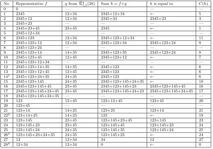
Proof. Like in Section 3, in order to prove the statement it is enough to show that for anyi = 1,2,3,4 and any EA-equivalence class C of F322 of even weight (other thanR1,5) there exists a functionf∈C and a functiong∈Rbi1,5such that f+g /∈Rb1,5. The proof for this can be found in the appendix in Tables 2-5. ut
Theorem 3 The codeR2,6 is metrically regular.
Proof. Since any linear code is a subset of its second metric complement, we only
need to prove that b b
R2,6 ⊆ R2,6. Let (u,˜ u˜+v˜) be a vector from Rbb2,6. We have already proved that˜uis inR2,5, therefore the vector (0,˜v) is also inRbb2,6. Let us prove that˜vis inR1,5.
Assume that ˜v ∈ R/ 1,5. Since (by Lemma 9) for an arbitrary (y,w) ∈Rb2,6 there exists a vector u ∈ R2,5 such that (w+u)∈Rb1,5, for some ithe second statement of Lemma 11 must hold.
By the second statement of Lemma 11, for thisw∗there exists a vector (y,w)∈ b
R2,6 and a vectoru∈ R2,5 such that (d(y,u) = 6∧w+u=w∗). Since (0,˜v)∈
b b
R2,6, (y,w+˜v) is also in Rb2,6, and since d(y,u) = 6, by Lemma 9 the vector
w+v˜+uis in Rb1,5. Butw+v˜+u=v˜+w∗∈/Rb1,5, contradiction. Therefore,
˜
v∈ R1,5 and hence (u,˜ u˜+v˜)∈ R2,6. ut
10 Conclusion
In this paper we have established the metric regularity of the codes RM(1,5),
RM(2,6) and of the codes RM(k, m) for k > m−3. Factoring in the result by Tokareva [16], which proves the metric regularity of RM(1, m) for even m, all infinite families of Reed-Muller codes with known covering radius are covered. The only other Reed-Muller codes with known covering radius, metric regularity of which has not been yet established, areRM(1,7) andRM(2,7). Given these results, we formulate the following
Conjecture. All Reed-Muller codesRM(k, m)are metrically regular.
The availability of the coset weight distributionfor allowed us to consider the code RM(1,5), and the fact that the covering radius of RM(2,6) attains an upper bound given by the (u,u+v) construction [14] allowed us to establish its metric regularity even without describing the metric complement. However, the codesRM(1,7) andRM(2,7) are much harder to consider because of the lack of similar regularities, the larger number of variables, the larger covering radius and the unconstructive nature of the results which describe their covering radius.
I would like to thank Natalia Tokareva, Alexander Kutsenko and the collective of the Selmer Center of the University in Bergen for the inspiration and helpful remarks during the development of this work.
References
1. Berlekamp E., Welch L.: Weight distributions of the cosets of the (32,6) Reed-Muller code. IEEE Transactions on Information Theory.18(1), 203–207 (1972).
2. Cohen G., Honkala I., Litsyn S., Lobstein A.: Covering codes. Elsevier.54, (1997). 3. Hou X. D.: Covering Radius of the Reed-Muller codeR(1,7) – A Simpler Proof. Journal of
Combinatorial Theory, Series A.74(2), 337–341 (1996).
4. Kolomeec N.: The graph of minimal distances of bent functions and its properties. Designs, Codes and Cryptography.85(3), 395–410 (2017).
5. Kutsenko A.: Metrical properties of self-dual bent functions. Designs, Codes and Cryptog-raphy (2019). doi:10.1007/s10623-019-00678-x
6. McLoughlin A. M.: The Covering Radius of the (m−3)-rd Order Reed Muller Codes and a Lower Bound on the (m−4)-th Order Reed Muller Codes. SIAM Journal on Applied Mathematics.37(2), 419–422 (1979).
7. Mesnager S.: Bent Functions: Fundamentals and Results. Springer International Publishing, (2016).
8. Mykkeltveit J.: The covering radius of the (128,8) Reed-Muller code is 56. IEEE Transac-tions on Information Theory.26(3), 359–362 (1980).
9. Neumaier A.: Completely regular codes. Discrete mathematics.106, 353–360 (1992). 10. Oblaukhov A. K.: Metric complements to subspaces in the Boolean cube. Journal of
Ap-plied and Industrial Mathematics.10(3), 397–403 (2016).
12. Oblaukhov A.: A lower bound on the size of the largest metrically regular subset of the Boolean cube. Cryptography and Communications.11(4), 777–791 (2019).
13. Rothaus O. S.: On “bent” functions. Journal of Combinatorial Theory, Series A.20(3), 300–305 (1976).
14. Schatz J.: The second order Reed-Muller code of length 64 has covering radius 18. IEEE Transactions on Information Theory.27(4), 529–530 (1981).
15. Stanica P., Sasao T., Butler J. T.: Distance duality on some classes of Boolean functions. Journal of Combinatorial Mathematics and Combinatorial Computing. 2018.
16. Tokareva N. N.: The group of automorphisms of the set of bent functions. Discrete Math-ematics and Applications.20(5–6), 655–664 (2010).
17. Tokareva N.: Duality between bent functions and affine functions. Discrete Mathematics.
312(3), 666–670 (2012).
18. Tokareva N.: Bent functions: results and applications to cryptography. Academic Press, (2015).
19. Wang Q.: The covering radius of the Reed–Muller codeRM(2,7) is 40. Discrete Mathe-matics.342(12), Article 111625 (2019).
Appendix
Tables 2-5 show that for any EA-equivalence classRbi1,5 ofRb1,5and for each EA-equivalence classC ofF322 there exists a functionf ∈C and a function g∈Rbi1,5 such that f+g does not belong toRb1,5. Note that, if this function f is not in
b
R1,5 andf+gbelongs to a classC0, then we do not have to search for a function with such properties in the classC0since (f+g) +g=f does not belong toRb1,5 — this is why some rows in the following tables are skipped.
Notations in Tables 2-5 are the same as in Table 1 (see Section 3). The second column of Table 5 contains “canonical” representatives for each EA-equivalence class, as they were obtained in the paper [1] by Berlekamp and Welch. In other columns and tables, some representatives are changed by either simple variable swaps or more complex transformations. These more complex transformations are marked with an asterisk and explained below for each table, along with other clarifications. Hereafter “i←i+j” stands for “xi←xi+xj”, while two-way arrows denote variable swapping; all transformations are applied consecutively.
Table 2:Representativesf for classes 7, 9, 10 and 22 (column 2) are obtained from “canonical” using the following transformations:
(7) 3←3+0; (9) 4←4+3+0; (10) 1←1+0; (22) 4↔5; 1↔3;
FunctionsgfromRb11,5(third column) are obtained from “canonical” using
trans-formations:
2345+123+24+35◦(2←2+0) = 2345+345+123+13+24+35; 2345+123+24+35◦(5←5+0) = 2345+234+123+24+35; 2345+123+24+35◦(1←1+0) = 2345+123+24+35+23;
Transformations which produce function in column 5 fromh in column 4: (1) 2←2+0; 4←4+0; 1↔3; (2) 2←2+0; 4←4+0; 1←1+4; 3←3+0; 5←5+2; 1↔3; 2↔4; 3↔5; (3) 1↔3; 4↔5; (5) 3←3+0; 1↔2; (6) 3←3+0; 1↔3; 3↔4; 4↔5; (7) 5←5+0; 1↔5; 3↔4; (8) 1↔3; 2↔5; (9) 4←4+0; 1←1+2; 1↔4; 2↔5;
Table 3:FunctionsgfromRb21,5(third column) are obtained from “canonical”
using variable swaps. Transformations which produce function in column 5 from
hin column 4:
(1) 2↔3; (2) 4←4+2+0; 2↔3; (3) 1←1+0; 2↔3; (4) 3←3+2+0; 1←1+2+3; (7) 4←4+2+0; 2↔4; 3↔5; (8) 2↔4; (10) 2←2+4+0; 2↔4; 3↔5; (11) 2←2+5+0; (13) 2←2+5+0; 5←5+3+0; 3↔5; (15) 2↔4; 3↔5; (16) 1←1+0; 2↔4; 3↔5; (17) 1←1+0; 2↔5; 3↔4; (18) 2↔4; 3↔5; (19) 3←3+0; 1↔5; (21) 1↔5;
(23) 5←5+0; 1↔5; 2↔4; 3↔5; (24) 5←5+0; 3←3+5; 2↔4; 3↔5; (25) 4←4+0; 2↔4; 3↔5; (26) 4←4+0; 2←2+5; 2↔4; 3↔5; (27) 1↔2; 4↔5;
Table 4: Representativesf for classes 4 and 9 (column 2) are obtained from “canonical” using the following transformations: (4) 3←3+0; (9) 1←1+2;
FunctionsgfromRb31,5(third column) are obtained from “canonical” using
trans-formations:
123+145+23+24+35◦(1←1+2) = 123+145+245+24+35; 123+145+245+24+35◦(3←3+0) = 123+145+245+24+35+12; 123+145+245+24+35+12◦(4↔5) = 123+145+245+25+34+12; 123+145+245+24+35+12◦(2↔4; 3↔5) = 123+145+234+24+35+14; 123+145+23+24+35◦(2↔4; 3↔5) = 123+145+45+24+35;
Transformations which produce function in column 5 fromh in column 4: (1) 3←3+0; (2) 3←3+0; (4) 1←1+0; (5) 1←1+2; 1←1+0; (6) 2←2+5+0; 3←3+4+0; 1←1+0; 2↔4; 3↔5; (7) 3←3+4; 1←1+4; 2↔4; 3↔5; (8) 2←2+5+0; 2↔4; 3↔5; (9) 5←5+0; 2←2+5+0; 2↔4; 3↔5; (11) 3←3+2; 2↔4; 3↔5; 2↔3; (14) 2↔4; 3↔5; (15) 5←5+2+0; 3↔4; (16) 3↔4; (17) 4←4+3+0; (19) 1←1+0; 3←3+4; 2←2+5; 2↔4; 3↔5; (21) 3←3+0; 1↔4; 2↔3; 4↔5; (22) 5←5+0; 2←2+4; 2↔4; 3↔5; (23) 5←5+0; 1↔5; 3↔4; (24) 5←5+0; 5←5+2+0; 1↔5; 3↔4;
(27) 5←5+2; 1←1+0; 3←3+4;
Table 5:FunctionsgfromRb41,5(third column) are obtained from “canonical”
using variable swaps. Transformations which produce function in column 5 from
hin column 4:
No Representativef gfromRb11,5(14) Sumh=f+g his equal to C(h)
0 0 — — — —
1 2345 2345+345+123+13+24+35 123+345+13+24+35 123+145+24 25
2 2345+12 2345+345+123+13+24+35 123+345+12+13+24+35 123+145+23 24
3 2345+24 2345+123+24+35 123+35 123+14 21
4 2345+24+35 2345+123+24+35 123 ← 19
5 2345+12+35 2345+123+24+35 123+12+24 123+14 21
6 2345+123 2345+234+123+24+35 234+24+35 123+14 21
7 2345+245+123∗ 2345+123+24+35 245+24+35 123+14 21
8 2345+123+24 2345+123+24+35 35 12 27
9 2345+123+14+13∗ 2345+345+123+13+24+35 345+14+24+35 123+14 21
10 2345+123+45+23∗ 2345+123+24+35 23+24+35+45 12 27
11 2345+123+12+35 2345+123+24+35 12+24 12 27
12 2345+123+14+35 2345+123+24+35 14+24 12 27
13 2345+123+13+45 2345+345+123+13+24+35 345+24+35+45 123+14 21
141 2345+123+24+35 2345+123+24+35 0 ← 0
15 2345+123+145 2345+234+123+24+35 145+234+24+35 123+145+24 25
16 2345+123+145+45 2345+234+123+24+35 145+234+24+35+45 123+145+24 25
17 2345+123+145+24+45 2345+123+24+35 145+45+35 123+14 21
18 2345+123+145+24+35 2345+123+24+35 145 123 19
19 123 — — — —
20 123+45 2345+123+24+35 2345+24+35+45 2345+23+45 4
21 123+14 — — — —
222 123+24+35∗ 2345+123+24+35 2345 ← 1
23 123+145 2345+123+24+35+23 2345+145+24+35+23 2345+123+45 10
24 123+145+23 2345+123+24+35 2345+145+24+35+23 2345+123+45 10
25 123+145+24 — — — —
263 123+145+23+24+35 2345+123+24+35 2345+145+23 2345+123+45 10
27 12 — — — —
284 24+35 2345+123+24+35 2345+123 ← 6
Table 2 Proof of Lemma 12 for the classRb11,5.
No Representativef gfromRb21,5(22) Sumh=f+g his equal to C(h)
0 0 — — — —
1 2345 123+14+25 2345+123+14+25 2345+123+14+35 12 2 2345+12 123+14+25 2345+123+12+14+25 2345+123+14+35 12 3 2345+23 123+14+25 2345+123+23+14+25 2345+123+14+35 12 4 2345+25+34 123+14+25 2345+123+14+34 2345+123+14 9 5 2345+14+25 123+14+25 2345+123 ← 6
6 2345+123 — — — 21
7 2345+123+12 123+14+25 2345+12+14+25 2345+12+34 5 8 2345+123+25 123+14+25 2345+14 2345+12 2
9 2345+123+14 — — — 21
10 2345+123+45 123+14+25 2345+14+25+45 2345+12+34 5 11 2345+123+12+34 123+15+34 2345+12+15 2345+12 2
12 2345+123+14+35 — — — 27
13 2345+123+12+45 123+15+34 2345+12+15+45+34 2345+12+34 5 141 2345+123+24+35 123+24+35 2345 ← 1
15 2345+123+145 123+14+25 2345+145+14+25 2345+12+34 11 16 2345+123+145+45 123+14+25 2345+145+14+25+45 2345+12+34 11 17 2345+123+145+24+45 123+24+35 2345+145+35+45 2345+123+24 8 18 2345+123+145+24+35 123+24+35 2345+145 2345+123 6 19 123+235 123+14+25 235+14+25 123+45 20
20 123+45 — — — —
21 123+14 123+14+25 25 12 27
222 123+14+25 123+14+25 0 ← 0
23 123+145 123+14+25 145+14+25 123+14 21 24 123+145+23 123+14+25 145+14+25+23 123+45 20 25 123+145+24 123+15+24 145+15 123 19 263 123+145+23+24+35 123+15+24 145+15+23+35 123+45 20
27 14 123+14+25 123+25 123+14 21
284 14+25 123+14+25 123 ← 19