Fast, Greedy Model Minimization for Unsupervised Tagging

Fast, Greedy Model Minimization for Unsupervised Tagging

Sujith Ravi and Ashish Vaswani and Kevin Knight and David Chiang

University of Southern California Information Sciences Institute

{sravi,avaswani,knight,chiang_}@isi.edu

Abstract

Model minimization has been shown to work well for the task of unsupervised part-of-speech tagging with a dictionary. In (Ravi and Knight, 2009), the authors in-voke an integer programming (IP) solver to do model minimization. However, solving this problem exactly using an integer programming formulation is in-tractable for practical purposes. We pro-pose a novel two-stage greedy approxima-tion scheme to replace the IP. Our method runs fast, while yielding highly accurate tagging results. We also compare our method against standard EM training, and show that we consistently obtain better tagging accuracies on test data of varying sizes for English and Italian.

1 Introduction

The task of unsupervised part-of-speech (POS) tagging with a dictionary as formulated by Meri-aldo (1994) is: given a raw word sequence and a dictionary of legal POS tags for each word type, tag each word token in the text. A common ap-proach to modeling such sequence labeling prob-lems is to build a bigram Hidden Markov Model (HMM) parameterized by tag-bigram transition probabilities P(ti|ti−1) and word-tag emission probabilitiesP(wi|ti). Given a word sequencew and a tag sequencet, of lengthN, the joint prob-abilityP(w, t)is given by:

P(w, t) =

N

Y

i=1

P(wi|ti)·P(ti|ti−1) (1)

We can train this model using the Expectation Maximization (EM) algorithm (Dempster and Ru-bin, 1977) which learnsP(wi|ti) andP(ti|ti−1) that maximize the likelihood of the observed data. Once the parameters are learnt, we can find the best tagging using the Viterbi algorithm.

ˆ

t= arg max

t

P(w, t) (2)

• We present an efficient two-phase greedy-selection method for solving the minimiza-tion objective from Ravi and Knight (2009), which runs much faster than their IP.

• Our method easily scales to large data sizes (and big tagsets), unlike the previ-ous minimization-based approaches and we show runtime comparisons for different data sizes.

• We achieve very high tagging accuracies

comparable to state-of-the-art results for un-supervised POS tagging for English.

• Unlike previous approaches, we also show results obtained when testing on the entire Penn Treebank data (973k word tokens) in addition to the standard 24k test data used for this task. We also show the effectiveness of this approach for Italian POS tagging.

2 Previous work

There has been much work on the unsupervised part-of-speech tagging problem. Goldwater and Griffiths (2007) also learn small models employ-ing a fully Bayesian approach with sparse pri-ors. They report 86.8% tagging accuracy with manual hyperparameter selection. Smith and Eis-ner (2005) design a contrastive estimation tech-nique which yields a higher accuracy of 88.6%. Goldberg et al. (2008) use linguistic knowledge to initialize the the parameters of the HMM model prior to EM training. They achieve 91.4% ac-curacy. Ravi and Knight (2009) use a Minimum Description Length (MDL) method and achieve the best results on this task thus far (91.6% word token accuracy, 91.8% with random restarts for EM). Our work follows a similar approach using a model minimization component and alternate EM training.

Recently, the integer programming framework has been widely adopted by researchers to solve other NLP tasks besides POS tagging such as se-mantic role labeling (Punyakanok et al., 2004), sentence compression (Clarke and Lapata, 2008), decipherment (Ravi and Knight, 2008) and depen-dency parsing (Martins et al., 2009).

3 Model minimization formulated as a Path Problem

The complexity of the model minimization step in (Ravi and Knight, 2009) and its proposed ap-proximate solution can be best understood if we formulate it as a path problem in a graph.

Letw= w0, w1, . . . , wN, wN+1 be a word se-quence wherew1, . . . , wN are the input word to-kens and{w0, wN+1} are the start/endtokens. LetT ={T1, . . . , TK}S{T0, TK+1}be the fixed set of all possible tags. T0 andTK+1 are special tags that we add for convenience. These would be thestartandendtags that one typically adds to

the HMM lattice. The tag dictionaryDcontains

entries of the form (wi, Tj) for all the possible tagsTj that word tokenwi can have. We add en-tries(w0, T0)and(wK+1, TK+1)toD. Given this input, we now create a directed graph G(V, E). LetC0, C1. . . , CK+1 be columns of nodes inG, where columnCi corresponds to word token wi. For alli= 0, . . . , N+1andj= 0, . . . , K+1, we add nodeCi,jin columnCiif(wi, Tj)∈D. Now,

∀i= 0, . . . , N, we create directed edges from

ev-ery node in Ci to every node in Ci+1. Each of these edgese = (Ci,j, Ci+1,k)is given the label

(Tj, Tk)which corresponds to a tag bigram. This creates our directed graph. Letl(e)be the tag

bi-gram label of edgese∈E. For every pathPfrom C0,0toCN+1,K+1, we say thatP uses an edge la-bel or tag bigram(Tj, Tk)if there exists an edge

ein P such that l(e) = (Tj, Tk). We can now formulate the the optimization problem as: Find the smallest setS of tag bigrams such that there

exists at least one path fromC0,0toCN+1,K+1 us-ing only the tag bigrams inS. Let us call this the

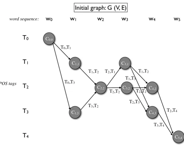
Minimal Tag Bigram Path (MinTagPath) problem. Figure 1 shows an example graph where the input word sequence is w1, . . . , w4 and T = {T1, . . . , T3} is the input tagset. We add the start/end word tokens {w0, w5} and correspond-ing tags{T0, T4}. The edges in the graph are in-stantiated according to the word/tag dictionaryD

T0

T1

T2

T3

T4

w0 w1 w2 w3 w4 w5

T0,T1

T0,T3

T1,T2 T2,T1 T1,T2

T2,T2

T3,T2

T3,T4

T2,T4

T2,T3

T2,T2

T1,T3

C0,0

C1,1

C1,3

C2,2

C3,1

C3,2 C4,2

C4,3

C5,4

word sequence:

POS tags

Initial graph: G (V, E)

Figure 1: Graph instantiation for the MinTagPath problem.

4 Problem complexity

Having defined the problem, we now show that it can be solved in polynomial time even though the number of paths from C0,0 to CN+1,K+1 is exponential inN, the input size. This relies on the

assumption that the tagset T is fixed in advance,

which is the case for most tagging tasks.1 _LetB

be the set of all the tag bigram labels in the graph,

B = {l(e),∀e∈ E}. Now, the size ofB would

be at mostK2+ 2K where every word could be

tagged with every possible tag. Form= 1. . ._|B_|,

let Bm be the set of subsets of B each of which

have size m. Algorithm 1 optimally solves the

MinTagPath problem.

Algorithm 1 basically enumerates all the possi-ble subsets ofB, from the smallest to the largest, and checks if there is a path. It exits the first time a path is found and therefore finds the smallest pos-sible set si of size msuch that a path exists that uses only the tag bigrams insi. This implies the

correctness of the algorithm. To check for path ex-istence, we could either throw away all the edges fromE not having a label insi, and then execute

a Breadth-First-Search (BFS) or we could traverse

1_{IfK, the size of the tagset, is a variable as well, then we}

suspect the problem is NP-hard.

Algorithm 1Brute Force solution to MinTagPath form= 1to|B_|do

forsi∈ Bmdo

Use Breadth First Search (BFS) to check if∃pathP fromC0,0toCN+1,K+1using only the tag bigrams insi.

ifP existsthen return si, m end if

end for end for

only the edges with labels insi during BFS. The running time of Algorithm 1 is easy to calculate. Since, in the worst case we go over all the sub-sets of sizem = 1, . . . ,|B|ofB, the number of

iterations we can perform is at most2|B|, the size

of the powersetP ofB. In each iteration, we do a BFS through the lattice, which hasO(N) time

complexity2 _{since the lattice size is linear in N}

and BFS is linear in the lattice size. Hence the run-ning time is≤2|B|·O(N) =O(N). Even though

this shows that MinTagPath can be solved in poly-nomial time, the time complexity is prohibitively large. For the Penn Treebank, K = 45 and the

worst case running time would be≈ 1013.55·N.

Clearly, for all practical purposes, this approach is intractable.

5 Greedy Model Minimization

We do not know of an efficient, exact algorithm to solve the MinTagPath problem. Therefore, we present a simple and fast two-stage greedy ap-proximation scheme. Notice that an optimal path

P (or any path)coversall the input words i.e.,

ev-ery word tokenwihas one of its possible taggings inP. Exploiting this property, in the first phase,

we set our goal to cover all the word tokens using the least possible number of tag bigrams. This can be cast as a set cover problem (Garey and John-son, 1979) and we use the set cover greedy ap-proximation algorithm in this stage. The output tag bigrams from this phase might still not allow any path fromC0,0toCN+1,K+1. So we carry out a second phase, where we greedily add a few tag bigrams until a path is created.

5.1 Phase 1: Greedy Set Cover

In this phase, our goal is to cover all the word to-kens using the least number of tag bigrams. The covering problem is exactly that of set cover. Let

U ={w0, . . . , wN+1}be the set of elements that needs to be covered (in this case, the word tokens). For each tag bigram (Ti, Tj) ∈ B, we define its corresponding covering setSTi,Tj as follows:

STi,Tj = {wn : ((wn, Ti)∈D

∧(Cn,i, Cn+1,j)∈E

∧l(Cn,i, Cn+1,j) = (Ti, Tj))

_

((wn, Tj)∈D

∧(Cn−1,i, Cn,j)∈E

∧l(Cn−1,i, Cn,j) = (Ti, Tj))}

Let the set of covering sets be X. We assign

a cost of1 to each covering set in X. The goal

is to select a set CHOSEN ⊆ X such that

S

S_Ti,Tj∈CHOSEN =U, minimizing the total cost

ofCHOSEN. This corresponds to covering all

the words with the least possible number of tag bigrams. We now use the greedy approximation algorithm for set cover to solve this problem. The pseudo code is shown in Algorithm 2.

Algorithm 2Set Cover : Phase 1 Definitions

DefineCAN D: Set of candidate covering sets in the current iteration

Define Urem : Number of elements in U re-maining to be covered

DefineES_Ti,Tj : Current effective cost of a set DefineItr: Iteration number

Initializations

LETCAN D=X

LETCHOSEN =_∅

LETUrem =U LETItr= 0

LETES_Ti,Tj = _|S 1

Ti,Tj|,∀STi,Tj ∈CAN D

whileUrem6=∅do

Itr_←Itr+ 1

Define_Sˆ_{Itr = argmin}

S_Ti,Tj∈CAN D

ES_Ti,Tj

CHOSEN = CHOSEN S SˆItr

Remove_Sˆ_{ItrfromCAN D}

Remove all the current elements in_Sˆ_Itrfrom Urem

Remove all the current elements in_Sˆ_Itrfrom

everySTi,Tj ∈CAN D

Update effective costs, ∀STi,Tj ∈ CAN D,

ES_Ti,Tj = _|S 1

Ti,Tj|

end while

return CHOSEN

For the graph shown in Figure 1, here are a few possible covering setsSTi,Tj and their initial

ef-fective costsES_Ti,Tj.

• ST0,T1 ={w0, w1},EST0,T1 = 1/2

• ST1,T2 ={w1, w2, w3, w4},EST₁,T₂ = 1/4

• ST2,T2 ={w2, w3, w4},EST₂,T₂ = 1/3

In every iterationItrof Algorithm 2, we pick a

set_Sˆ_{Itr that is most cost effective. The elements}

that_Sˆ_{Itrcovers are then removed from all the}

re-maining candidate sets and Urem and the effec-tiveness of the candidate sets is recalculated for the next iteration. The algorithm stops when all elements of U i.e., all the word tokens are

CHOSEN}, be the set of tag bigrams that have been chosen by set cover. Now, we check, using BFS, if there exists a path fromC0,0toCN+1,K+1 using only the tag bigrams inBCHOSEN. If not,

then we have to add tag bigrams toBCHOSEN to enable a path. To accomplish this, we carry out the second phase of this scheme with another greedy strategy (described in the next section).

For the example graph in Figure 1, one possible solution BCHOSEN =

{(T0, T1),(T1, T2),(T2, T4)}.

5.2 Phase 2: Greedy Path Completion

We define a graph GCHOSEN(V0, E0) ⊆

G(V, E) that contains the edges e ∈ E such l(e)_∈BCHOSEN.

LetBCAN D = B\BCHOSEN, be the current set of candidate tag bigrams that can be added to the final solution which would create a path. We would like to know how manyholesa particular

tag bigram(Ti, Tj)can fill. We define a hole as an edgeesuch thate ∈ G\GCHOSEN and there exists e0, e00 ∈ GCHOSEN such that tail(e0) =

head(e) _∧ tail(e) =head(e00).

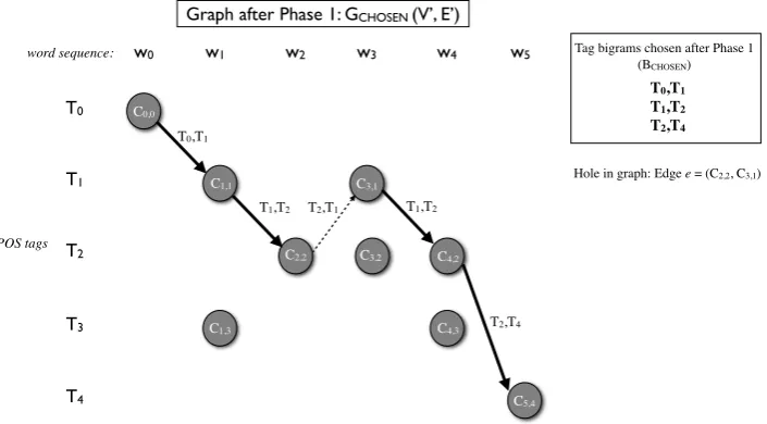
Figure 2 illustrates the graphGCHOSEN using tag bigrams from the example solution to Phase 1 (Section 5.1). The dotted edge (C2,2, C3,1) rep-resents a hole, which has to be filled in the cur-rent phase in order to complete a path from C0,0 toC5,4.

In Algorithm 3, we define the effectiveness of a candidate tag bigramH(Ti, Tj)to be the number of holes it covers. In every iteration, we pick the most effective tag bigram, fill the holes and recal-culate the effectiveness of the remaining candidate tag bigrams.

Algorithm 3 returns BF IN AL, the final set of

chosen tag bigrams. It terminates when a path has been found.

5.3 Fitting the Model

Once the greedy algorithm terminates and returns a minimized grammar of tag bigrams, we follow the approach of Ravi and Knight (2009) and fit the minimized model to the data using the alter-nating EM strategy. The alteralter-nating EM iterations are terminated when the change in the size of the observed grammar (i.e., the number of unique tag

Algorithm 3Greedy Path Complete : Phase 2 DefineBF IN AL : Final set of tag bigrams se-lected by the two-phase greedy approach

LETBF IN AL=BCHOSEN

LET H(Ti, Tj) = |{e}| such that l(e) =

(Ti, Tj)andeis a hole,∀(Ti, Tj)∈BCAN D

while@ pathP fromC0,0 toCN+1,K+1 using only(Ti, Tj)∈BCHOSEN do

Define( ˆTi,Tˆj) = argmax (Ti,Tj)∈BCAN D

H(Ti, Tj)

BF IN AL = BF IN AL S( ˆTi,Tˆj) Remove( ˆTi,Tˆj)fromBCAN D

GCHOSEN = GCHOSENS{e} such that

l(e) = (Ti, Tj)

∀(Ti, Tj)∈BCAN D, RecalculateH(Ti, Tj) end while

return BF IN AL

bigrams in the tagging output) is≤5%. We refer

to our entire approach using greedy minimization followed by EM training as MIN-GREEDY.

6 Experiments and Results 6.1 English POS Tagging

Data: We use a standard test set (consisting of 24,115 word tokens from the Penn Treebank) for the POS tagging task (described in Section 1). The tagset consists of 45 distinct tag labels and the dictionary contains 57,388 word/tag pairs derived from the entire Penn Treebank. Per-token ambi-guity for the test data is about 1.5 tags/token. In addition to the standard 24k dataset, we also train and test on larger data sets of 48k, 96k, 193k, and the entire Penn Treebank (973k).

Methods: We perform comparative evaluations for POS tagging using three different methods:

1. EM: Training a bigram HMM model using EM algorithm.

2. IP: Minimizing grammar size using inte-ger programming, followed by EM training (Ravi and Knight, 2009).

Sec-T0

T1

T2

T3

T4

w0 w1 w2 w3 w4 w5

T0,T1

T1,T2 T2,T1 T1,T2

T2,T4 C0,0

C1,1

C1,3

C2,2 C3,1

C3,2 C4,2

C4,3

C5,4 word sequence:

POS tags

T0,T1 T1,T2 T2,T4 Tag bigrams chosen after Phase 1

(BCHOSEN)

Hole in graph: Edge e = (C2,2, C3,1)

Graph after Phase 1: GCHOSEN (V’, E’)

Figure 2: Graph constructed with tag bigrams chosen in Phase 1 of the MIN-GREEDY method.

tion 5, followed by EM training.

Results: Figure 3 shows the tagging perfor-mance (word token accuracy %) achieved by the three methods on the standard test (24k tokens) as well as Penn Treebank test (PTB = 973k tokens). On the 24k test data, the MIN-GREEDY method achieves a high tagging accuracy comparable to the previous best from the IP method. However, the IP method does not scale well which makes it infeasible to run this method in a much larger data setting (the entire Penn Treebank). MIN-GREEDY on the other hand, faces no such prob-lem and in fact it achieves high tagging accuracies on all four datasets, consistently beating EM by significant margins. When tagging all the 973k word tokens in the Penn Treebank data, it pro-duces an accuracy of 87.1% which is much better than EM (82.3%) run on the same data.

Ravi and Knight (2009) mention that it is pos-sible to interrupt the IP solver and obtain a sub-optimal solution faster. However, the IP solver did not return any solution when provided the same amount of time as taken by MIN-GREEDY for any of the data settings. Also, our algorithms were implemented in Python while the IP method employs the best available commercial software package (CPLEX) for solving integer programs.

Figure 4 compares the running time efficiency for the IP method versus MIN-GREEDY method

Test set Efficiency

(average running time in secs.)

IP MIN-GREEDY

24k test 93.0 34.3

48k test 111.7 64.3

96k test 397.8 93.3

193k test 2347.0 331.0

PTB (973k) test ∗ _1485.0

Figure 4: Comparison of MIN-GREEDY versus MIN-GREEDY approach in terms of efficiency (average running time in seconds) for different data sizes. All the experiments were run on a sin-gle machine with a 64-bit, 2.4 GHz AMD Opteron 850 processor.

Method Tagging accuracy (%) when training & testing on: 24k 48k 96k 193k PTB (973k)

EM 81.7 81.4 82.8 82.0 82.3

IP 91.6 89.3 89.5 91.6 ∗

MIN-GREEDY 91.6 88.9 89.4 89.1 87.1

Figure 3: Comparison of tagging accuracies on test data of varying sizes for the task of unsupervised English POS tagging with a dictionary using a 45-tagset. (∗_{IP method does not scale to large data).}

400 600 800 1000 1200 1400 1600

Observed grammar size (# of tag bigrams)

in final tagging output

Size of test data (# of word tokens)24k 48k 96k 193k PTB (973k)

EM IP Greedy

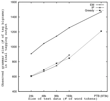
Figure 5: Comparison of observed grammar size (# of tag bigram types) in the final tagging output from EM, IP and MIN-GREEDY.

more than 3 hours without returning a solution. It is interesting to see that for the 24k dataset, the greedy strategy finds a grammar set (contain-ing only 478 tag bigrams). We observe that MIN-GREEDY produces 452 tag bigrams in the first minimization step (phase 1), and phase 2 adds an-other 26 entries, yielding a total of 478 tag bi-grams in the final minimized grammar set. That is almost as good as the optimal solution (459 tag bigrams from IP) for the same problem. But MIN-GREEDY clearly has an advantage since it runs much faster than IP (as shown in Figure 4). Figure 5 shows a plot with the size of the ob-served grammar (i.e., number of tag bigram types in the final tagging output) versus the size of the test data for EM, IP and MIN-GREEDY methods. The figure shows that unlike EM, the other two approaches reduce the grammar size considerably and we observe the same trend even when scaling

Test set Average Speedup Optimality Ratio

24k test 2.7 0.96

48k test 1.7 0.98

96k test 4.3 0.98

193k test 7.1 0.93

Figure 6: Average speedupversusOptimality ra-tio computed for the model minimization step (when using MIN-GREEDY over IP) on different datasets.

to larger data. Minimizing the grammar size helps remove many spurious tag combinations from the grammar set, thereby yielding huge improvements in tagging accuracy over the EM method (Fig-ure 3). We observe that for the 193k dataset, the final observed grammar size is greater for IP than MIN-GREEDY. This is because the alternating EM steps following the model minimization step add more tag bigrams to the grammar.

We compute the optimality ratio of the MIN-GREEDY approach with respect to the grammar size as follows:

Optimality ratio = Size of IP grammar

Size of MIN-GREEDY grammar

Method Tagging accuracy (%) Number of unique tag bigrams in final tagging output

EM 83.4 1195

IP 88.0 875

MIN-GREEDY 88.0 880

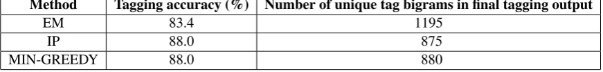
Figure 7: Results for unsupervised Italian POS tagging with a dictionary using a set of 90 tags.

take on all tag labels. In such cases, we can fol-low a similar approach as Ravi and Knight (2009) to assign tag possibilities to every unknown word using information from the known word/tag pairs present in the dictionary. Once the completed dic-tionary is available, we can use the procedure de-scribed in Section 5 to minimize the size of the grammar, followed by EM training.

6.2 Italian POS Tagging

We also compare the three approaches for Italian POS tagging and show results.

Data: We use the Italian CCG-TUT corpus (Bos et al., 2009), which contains 1837 sentences. It has three sections: newspaper texts, civil code texts and European law texts from the JRC-Acquis Multilingual Parallel Corpus. For our experi-ments, we use the POS-tagged data from the CCG-TUT corpus, which uses a set of 90 tags. We created a tag dictionary consisting of 8,733 word/tag pairs derived from the entire corpus (42,100 word tokens). We then created a test set consisting of 926 sentences (21,878 word tokens) from the original corpus. The per-token ambiguity for the test data is about 1.6 tags/token.

Results: Figure 7 shows the results on Italian POS tagging. We observe that MIN-GREEDY achieves significant improvements in tagging ac-curacy over the EM method and comparable to IP method. This also shows that the idea of model minimization is a general-purpose technique for such applications and provides good tagging ac-curacies on other languages as well.

7 Conclusion

We present a fast and efficient two-stage greedy minimization approach that can replace the inte-ger programming step in (Ravi and Knight, 2009). The greedy approach finds close-to-optimal solu-tions for the minimization problem. Our

algo-rithm runs much faster and achieves accuracies close to state-of-the-art. We also evaluate our method on test sets of varying sizes and show that our approach outperforms standard EM by a sig-nificant margin. For future work, we would like to incorporate some linguistic constraints within the greedy method. For example, we can assign higher costs to unlikely tag combinations (such as “SYM SYM”, etc.).

Our greedy method can also be used for solving other unsupervised tasks where model minimiza-tion using integer programming has proven suc-cessful, such as word alignment (Bodrumlu et al., 2009).

Acknowledgments

The authors would like to thank Shang-Hua Teng and Anup Rao for their helpful comments and also the anonymous reviewers. This work was jointly supported by NSF grant IIS-0904684, DARPA contract HR0011-06-C-0022 under sub-contract to BBN Technologies and DARPA con-tract HR0011-09-1-0028.

References

Bodrumlu, T., K. Knight, and S. Ravi. 2009. A new

objective function for word alignment. In

Proceed-ings of the NAACL/HLT Workshop on Integer Pro-gramming for Natural Language Processing.

Bos, J., C. Bosco, and A. Mazzei. 2009. Converting a dependency treebank to a categorial grammar

tree-bank for Italian. InProceedings of the Eighth

In-ternational Workshop on Treebanks and Linguistic Theories (TLT8).

Clarke, J. and M. Lapata. 2008. Global inference for sentence compression: An integer linear

program-ming approach. Journal of Artificial Intelligence

Research (JAIR), 31(4):399–429.

EM algorithm. Journal of the Royal Statistical So-ciety, 39(1):1–38.

Garey, M. R. and D. S. Johnson. 1979. Computers

and Intractability: A Guide to the Theory of NP-Completeness. John Wiley & Sons.

Goldberg, Y., M. Adler, and M. Elhadad. 2008.

EM can find pretty good HMM POS-taggers (when

given a good start). In Proceedings of the 46th

Annual Meeting of the Association for Computa-tional Linguistics: Human Language Technologies (ACL/HLT).

Goldwater, Sharon and Thomas L. Griffiths. 2007. A fully Bayesian approach to unsupervised

part-of-speech tagging. InProceedings of the 45th Annual

Meeting of the Association for Computational Lin-guistics (ACL).

Martins, A., N. A. Smith, and E. P. Xing. 2009. Con-cise integer linear programming formulations for

dependency parsing. In Proceedings of the Joint

Conference of the 47th Annual Meeting of the As-sociation for Computational Linguistics (ACL) and the 4th International Joint Conference on Natural Language Processing of the AFNLP.

Merialdo, B. 1994. Tagging English text with a

probabilistic model. Computational Linguistics,

20(2):155–171.

Punyakanok, V., D. Roth, W. Yih, and D. Zimak. 2004. Semantic role labeling via integer linear

pro-gramming inference. In Proceedings of the

Inter-national Conference on Computational Linguistics (COLING).

Ravi, S. and K. Knight. 2008. Attacking decipher-ment problems optimally with low-order n-gram

models. InProceedings of the Conference on

Em-pirical Methods in Natural Language Processing (EMNLP).

Ravi, S. and K. Knight. 2009. Minimized models

for unsupervised part-of-speech tagging. In

Pro-ceedings of the Joint Conference of the 47th An-nual Meeting of the Association for Computational Linguistics (ACL) and the 4th International Joint Conference on Natural Language Processing of the AFNLP.