Spatial analysis of points on tree structures: the distribution of epiphytes on tropical trees

.e

7he Library of the Department of

Statistics

~Drth

Carolina State University

SPATIAL ANALYSIS OF POINTS ON TREE STRUCTURES: THE DISTRIBUTION OF EPIPHYTES ON TROPICAL TREES

Douglas Nychka1 Nalini Nadkarni2

Institute of Statistics Mimeograph Series No. 1971

.e

Spatial analysis of points on tree structures:

the distribution of epiphytes on tropical trees

Douglas Nychka1

Nalini Nadkarni2 December 18, 1989

A frequent problem in ecology is determining whether the observed spatial distribution of a plant species can be attributed to a completely random spatial process. Usually the analysis of these data is simplified by the fact that the locations of the plants are the two-dimensional coordinates in a rectangular region. This paper considers a more difficult problem of assessing the spatial pattern of points that lie on a tree structure. The application in this work involves the distribution of a type of epiphyte found in the crowns of a group of tropical trees. These methods, however, are not limited to biological trees and could be useful for the spatial analysis of other treelike structures or networks.

A tree structure imposes complicated constraints on the three-dimensional relationships among different points on the network. For this reason it is not possi~leto obtain simple. analytical expressions for testing statistical hypotheses about the spatial distribution of the observed data. The basic idea behind our approach is to use Monte Carlo simulation of point patterns to test for spatial randomness in the observed data. One advantage of this approach is that it can handle spatial statistics that may be very relevant for a particular problem but may be too complicated to work with analytically.

Our spatial analysis of the bromeliads' distributions in tree crowns yields surprising results. The distribution of plants on different trees appear to depart from a completely random (uniform) pattern both in the direction toward clustering and also toward

hyperdispersion (regularity). These results suggest that there may be other factors besides the basic tree architecture that influence the distribution of epiphytes within tree crowns.

The analysis of the spatial distribution of epiphytes in tree crowns requires detailed knowledge of the three-dimensional structure of the tree crown and we believe this is the first instance where the structure of standing trees has been mapped. Because of the novelty of these data some discussion is given on the statistical issues of converting pairs of transit sitings to an xyz coordinate system.

Key Words and Phrases: Spatial statistics, Nearest neighbor distance statistic, Tree maps

IDouglas Nychka is an Associate Professor in the Department of Statistics at North

Carolina State University, Raleigh, NC 27695-8203

2Nalini Nadkarni is Director of Research at the Marie Selby Botanical Gardens,

.e

1 Introduction

Often botanical and ecological questions can be formulated in terms of the presence or

absence of spatial patterns. These data typically involve the positions or quadrat counts over a

two-dimensional rectangular region and many statistical methods have been developed for

interpreting such data (Ripley 1981, Diggle 1983). This article considers the extension of these

methods to analyze spatial point patterns that are constrained to lie on a tree-structure.

Although our application considers structures that are forest trees, there is the potential

application to other branching structures such as stream networks, circulatory systems and

neural pathways.

The canopy of a tropical rain forest is a rich and largely unexplored ecosystem that

plays a vital role in storing and recycling nutrients. Recently the canopy ecosystem has also

become an environmental concern. Given the rapid clearing of rain forest for agriculture and

grazing, it is important to understand how the destruction of the canopy will effect the

amount of nutrients left in the soil. In the past decade, understanding of the organisms and

interactions of tropical forest tree canopies has greatly increased due to the use of

mountain-climbing techniques for canopy access ( Nadkarni 1981, Perry 1984). A sound scientific

understanding of the canopy has been hindered, however, by the lack of quantitative data on

the distribution and abundance of canopy biota and on .the microenvironment of the canopy.

In order to study this ecosystem it is necessary to develop means for mapping tree structure

and locations of constituent organisms and to identify rigorous statistical methods to interpret

these data.

We have developed the capability to efficiently and inexpensively map individual tree

crowns, record associated dimensions and biota, and portray the resulting data graphically. In

this article we discuss the application of spatial statistics to study the distribution of

bromeliads a type of epiphyte that is supported by branches in the tree crown. Epiphytes

comprise a signifi"cant proportion of the tropical canopy biomass. Their ecological function is to

accumulate nutrients derived from atmospheric sources( Nadkarni 1984, 1986, Benzing 1989).

For this reason it important to understand the mechanisms that influence their abundance and

dispersion.

One way to appreciate the problems in analyzing tree structured data is to examine

the data collected for several trees. Figures 1 - 3 are the top and side projections of three of

the trees in this study along with the location of bromeliads. Such plots will be referred to as

tree maps. The basic question, given these data, is whether the locations of these plants depart

significantly from a completely random pattern. By completely random we mean that the

locations of the plants are independent of one another and, with respect to the top view, there

is an equal probability of being located anywhere on the tree network ( see Section 3 for more

discussion of this definition). Because plants are always located on branches, even a random

distribution of epiphytes will not appear uniformly distributed in space. This constraint makes

it difficult to interpret tree maps such as Figures 1-3 and visually assess the degree of

randomness. In fact, these three figures illustrate a range of possibilities for the spatial

distribution. For example, consider the median of the nearest neighbor distances (MNND)

among these plants. One way to interpret this statistic is to compare the observed value to a

reference distribution for this statistic based on the assumption of a completely random

distribution of points. For the tree in Figure 1 the MNND lies in the left tail of the reference

distribution, suggesting that these plants tend to cluster. The MNND for Figure 2 lies in the

right tail of the corresponding reference distribution and thus suggests that the bromeliad

locations tend to be hyperdispersed (or regular). The tree in Figure 3 is one where based on

the MNND statistic there is no evidence to reject the hypothesis of a completely random

distribution. Note that it is difficult visually to distinguish between the distribution of

bromeliads on these three trees even though the departures from pure randomness in the first

two cases are significant ( p-values .05 and .02 respectively). A characterization of the

e

epiphyte distributions from qualitative field observation would be even more difficult.

A statistical analysis of spatial data naturally breaks into two steps: 1) Testing for

departures from a purely random point pattern and 2) if departures are found, modeling the

point process using appropriate parametric distributions (Diggle 1983). The basic

computational tool used in the analysis is to simulate locations on a network of branches given

a specified distribution. Such simulated cases can be used to create a reference distribution for

a particular test statistic and to quantify how likely it is that the observed statistic came from

the specified distribution. This paper concentrates on the first phase of this analysis, because

the small sample sizes and heterogeneity of the data limit the amount of modeling. Fitting

parametric models in the second step, however, would use the same simulation methods

developed for the first part of the analysis. Besides statistical modeling, simulation methods

also have an important application in generating sampling designs for the tree crowns.

.e

In this paper we analyze the spatial distribution of tank bromeliads on a set of tropical

trees. In Section 2 we describe the determination of xyz coordinates for plant and branch

locations from pairs of transit sitings and the specific protocol used to collect the epiphyte

data. Due to the novelty of this measurement technique some discussion of the statistical

.e

properties of this method are also included. In Section 3 we review some principles for

analyzing spatial data and describe the specific methods used for the bromeliad locations.

Section 4 contains the results of testing for random point patterns in the bromeliad

distributions while Section 5 has a discussion of these results.

2 Three-dimensional trianCulation

JrWl.lM

collection

m

~ ~

gm

The basic measurement problem is to determine the 3-dimensional coordinates of a set

of points from a limited number of remote sites. One method is to locate the points of interest

by triangulation using pairs of transit measurements (Figure 4). The two transits are located

directly over two fixed reference points, RI and R2. Without any loss of generality, the

cartesian coordinate system may be oriented to have its origin at RI and for R2 to be located

"at the point (L,O,E). Here Lis the horizontal.distance between the reference points and E is the relative difference in elevation.Ifthere was no elevation difference between RI and R2, the

second reference point would lie on the positive X-axis a distance L from the origin. It is also

necessary to know the elevation of the transit center above each reference point and these will

be denoted by hI and h

2. The horizontal and azimuthal angles measured by the transits are assumed to have the same sense as () and <P in a spherical coordinate system. Sighting at the target from the first reference point yields the pair of angles «(}I,<PI) and in a similar manner

one obtains (02,<P2) from a transit situated over R2.

For each target location fourangular measurements are made even though the goal is

de~ermine only three coordinates. This extra angular measurement makes it possible to

determine the accuracy of the triangularization. Imagine the line of sights of the two transits

as rays that start from the transits and point to target. Ifthere were no error in sighting, then

the location of the target is the point where these two rays intersect. In practice the rays will

not intersect precisely, and under these circumstances it is reasonable to estimate the position

of the target as the location that is "closest" to both rays. Specifically, we find the shortest

line segment connecting these two rays and estimate the target's location by the midpoint of

this line segment. (The estimated location in Figure <1 is marked by an "X" .). A natural

estimate of the error is to report the length of this line segment and we will refer to this length

as the discrepancy. A formula for the estimated location and the discrepancy is derived in the

Appendix.

One might also consider estimating the position using nonlinear least squares or a

maximum likelihood estimate. Although these more sophisticated methods could be generalized

•

.e

measure of the discrepancy will not have such a clear geometric interpretation. One advantage

of our method is that the calculations can be done on a programmable calculator in the field.

Thus sightings that have a large discrepancy can be rechecked immediately while the transit is

still in position.

The sample trees in this study consisted of 12 individuals of Sapium oligoneuron

(Euphorbiaceae) located in a diary pasture near Monteverde, Costa Rica ( lO018'N, 84°48' W

). This study is the first in which the architecture of live tropical trees has been measured in a

precise, quantitative manner. Because we were developing a new field technique we chose trees

of simple structure and relatively small stature. Also these trees' open crowns and sparse

foliage permitted clear visibility from all angles in the surrounding flat grassland. Each tree

was mapped from two reference points a distance of 3 meters apart that were located roughly

10 meters from the trunk. A Topcon digital transit, accurate to 30 seconds of a degree, was

used to measure direction angles.

Any point on the tree of interest will be referred to as a node. In this study nodes are

all intersections, bends of the branches and the centers of the epiphytes. A tree skeleton is

constructed by appropriately connecting the nodes by straight line segments. Branches that

were smaller than 5 cm in diameter (visually estimated) were not mapped. Due to the

proximity of plants and branch forks sometimes a single node was taken as the location of

more than one feature. Each epiphyte was classified according to type ( bromeliad or mistletoe

) and relative size ( small, medium or large).

The largest source of error in mapping node locations was not in making the transit

measurements themselves, but in pairing sightings from the two reference points. To guard

against this problem, before mapping a tree a rough sketch was made of the tree that

highlights the connectivity information among the nodes. The 3 meter separation of the

reference points was a compromise between allowing for an accurate triangulation and making

it easy to identify the same node from two different perspectives. Nodes with a discrepancy of

more than .1 meters were omitted from the analysis.

Since it is possible to make gross errors in estimating node positions simply by

misidentifying them at one of the reference points it is important to consider a measure of

accuracy along with the estimated position. We chose to use the discrepancy although some

care needs to be taken in interpreting this value as an error estimate. This section ends by

quantifying the relationship between the calculated discrepancy and the actual error in the

estimate of a node's coordinates.

..

.e

Let 6 denote the distance between a node's estimated position and its true position

and let D denote the discrepancy. A series of simulations were run to study the distribution of

6/D as a function of different distances of the target from the transit base line. Like the field

work, the reference points in this simulation were separated by 3 meters but to simplify this

analysis we took them to be at the sameelevatio~and also located thetra~sitsat these points.

In practice, translating the coordinate system from the elevation of the transits to the

reference points does not generate any error. Constraining the transits to be at the same

elevation may improve the accuracy of this triangulation method but we believe this will be a

minor effect relative to the overall variability of the estimate. The nodes were located an equal

distance from the two reference points. This optimal placement may reduce the error but we

believe that the decrease in accuracy is not substantial provided the angular separation

between the reference points with respect to the node is comparable to the equidistant

position.

One difficulty of simulating transit measurement errors is that error in the horizontal

angles depend on the azimuthal angle. For example an error in the horizontal angle when the

azimuthal angle is zero is very different from the same error when the azimuthal angle is close

to 90 degrees. This does not reflect the actual measurement process because it is reasonable to

as~uinethat the transit may be pointed with equal accuracy in almost any direction. One way

of modeling this homogeneity is to locate all the node locations at the same elevation as the

transits, that is, the true azimuthal angle is 90 degrees. Equivalently one could assume that

the transit's base has been tilted so that the azimuthal angle for the node is at 90 degrees. For

such locations one way of approximating the measurement error is to add two independent,

N(O,y) random variables to the tru"e horizontal and azimuthal angles.

The distribution of (6/D) was studied at two levels of "'{ (.05,.2 ) and forty different

distances ranging from 5 to 20 meters. The two standard deviations levels are rough estimates

of the error in using a transit for finding the directions and the error from using a staff

compass and inclinometer. (Even though the digital transit has a nominal accuracy of 30

seconds, a more substantial error is incurred by not sighting on exactly the same point from

the two different perspectives.) The range of distances of the node to the reference points is

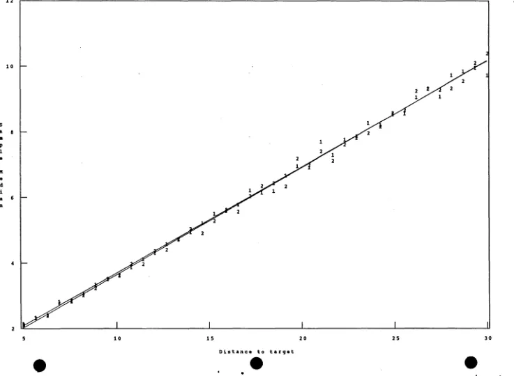
similar to those encountered in our tree mapping applications. Figure 5 is a plot of the

estimated 50 percentile for the distribution of 6/D as a function of the distance from the node

to the reference points. Also plotted are lines fit to these results using least squares. Each

percentile used in this plot was calculated from a random sample of 5000 observations. These

results show that D tends to be significantly smaller than 6 and this bias increases as the

-e

distance increases. Thus one should be cautious about interpreting the discrepancy literally as

the measurement error. One explanation for this bias is that 6 is result of minimizing the

distance between the two line of sights. Since 6 is being made as small as possible is not

surprising that it underestimates the true error. Two striking features of these results are the

linear dependence of the median on distance and -the insensitivity to the amount

of-measurement error. For field of-measurements that are within the range of the parameters of this

simulation one might use this approximate linear dependence to calculate a rough inflation

factor for the discrepancy measurement.

Section.a Spatial statistics for tree structures

This section will discuss methods for interpreting the spatial distribution of points.

These statistical problems have been widely studied for regular two dimensional regions

(Ripley 1981, Diggle 1983, Greg-Smith 1983) and the basic principles carryover for data

restricted to a network. Sterner, et al. (1985) give an example of these methods for

2-dimensional regions applied to the interaction between juvenile and adult tropical trees.

The first step in a spatial analysis is to test for departures of the point patterns from

complete spatial randomness (CSR). For a homogeneous two-dimensional region, such as a

quadrat of the forest floor, CSR is usually taken to be a Poisson process'with constant

intensity. Conditioning on the total number of points in the region, this process will yield

points whose locations are independent from one another and are uniformly distributed over

the region. The corresponding spatial process for a tree structure is one where points are

distributed uniformly along the branch segments. Because we are interested in plants being

supported by these branches, however, this distribution is not a reasonable one. Each branch

presents a certain amount of horizontal or near-horizontal surface area to serve as a platform

for the epiphyte. Even a random distribution of the plants should favor branches that present

a larger amount of surface area. To account for this constraint on the distribution of

epiphytes, we will define CSR to be the result of distributing points uniformly on the XY

projection of the tree structure. Specifically, the probability that a point will be located on a

particular branch will be proportional to the length of the branch when projected onto the XY

plane. Conditional on a point lying on a particular branch, the location will be uniformly

distributed between the two endpoints. In the context of our analysis, we will refer to this

stochastic point process as a completely random spatial process (CRSP). Details for efficiently

simulating this point process and more complicated ones are given at the end of this section.

CSR. These include the empirical distributions of interpoint distances, nearest neighbor

distances and point to nearest event distances. Out of these statistics, the nearest neighbor

distance (NND) seemed the most promising because of the sensitivity to clustering and also

because of its interpretability. From an biological point of view, it was appropriate to consider

the height of the bromeliad above the ground and the horizontal distance of the bromeliad

from the center or core of the tree crown. The approach suggested by Diggle (1983) is to

compare the empirical distribution of a particular statistic with the expected distribution of

the same statistic when point patterns are generated under the assumption of CSR. This

analysis was applied to the tree where the largest number of bromeliads (53) were observed.

Figure 6 is a plot of the empirical distribution of the nearest neighbor distances for the 53

bromeliad locations ( solid broken line) and the expected distribution function when the 53

locations are generated from a CRSP ( solid curved line) . In some very simple cases it is

possible to derive a closed form expression for the expected distribution function of a spatial

statistic under the hypothesis of CSR. In the case of processes restricted to a tree structure

this is usually not possible and one must resort to Monte Carlo simulation methods to

compute this distribution function. Along with computing the distribution function, one may

also find bounds that suggest the amount of variability that one would expect for the empirical

distribution function. These bounds are the dashed lines in Figure 6 and are the first and 99th

percentiles of the marginal distribution. They should be interpreted in the following manner:

For a fixed value the nearest neighbor distance, the probability that the empirical distribution

will be beyond either the upper or lower bound is .01.

Although one could consider hypothesis tests based directly on the empirical

distribution of a particular statistic, our analysis was restricted to either the mean or the

median of the observed distribution. Specifically, we considered the MNND, the average height

and the average crown distance as summary statistics for testing departures from CSR. This

reduction is appropriate given the small numbers of plants observed for each tree (see Table

1). The median was preferred over the average as a summary of the nearest neighbor distances

for two reasons. First, when epiphytes were observed to be close together 'on a branch these

plants were mapped to the same node. Thus some of the nearest neighbor distances are zero. A

median statistic is one simple way of making the hypothesis test insensitive to these artificial

zeroes in interplant distances. Second, since the distribution of statistics such as the nearest

neighbor distances is not known to be symmetric, the median seemed to be a more useful

summary of the distribution. Figure 7 is a histogram of 1000 simulated MNND statistics for

tree #9 under the hypothesis of CSR. Each value was generated by simulating 53 points on

e

the tree skeleton following a eSRP and then computing the MNND for these random locations. The arrow indicates the observed MNND for the data and is located at the 98th

percentile of these values. Thus considering a two sided alternative, the p-value for the test is

approximately .04 where the null hypothesis is rejected in the direction of a larger MNND.

Note that this result agrees with the more detailed analysis of the distribution described above.

Ripley (1979) discusses several other summary statistics that might be used to test for

eSR. Although his discussion is limited to rectangular, two-dimensional regions and it is easy

to extend these statistics to processes restricted to tree structures. His simulations indicate

that a class of V-statistics based on pairwise distances have much better power that the mean

NND for clustered patterns and a statistic of this form was included in our analysis to serve as

a benchmark. Let

~k

=(X_k1,X

k2,Xk3)T denote the estimated coordinates for the location of the kth bromeliad. Adding a third coordinate to the statistic referred to by Ripley as J let

J_{3 =}

Lq)(~k'~J')

k<j

where

q)(~k'~j) =1~1

(c-IXkl-Xjlj)+ and (u)+=u for

u~O

and 0 if u$O. To compute this

statistic we take c=MNND and evaluate the significance level using the same simulation

methods described above.

Besides testing for eSR individually for each. tree it is also important to consider how

to summarize the individual test results to draw conclusions about the pasture trees as a

group. Because tree crown architecture and the number of epiphytes varies among this sample,

many of the statistics summarizing the epiphyte distribution can not be compared across trees.

The p-values for the individual hypothesis tests were used as a way of standardizing the

results. One simple way of testing for an overall departure from eSR is to use the fact that

under the null hypothesis the p-values will have a uniform distribution on the interval [0,1].

Thus, we tested for departure from a uniform distribution using a X2goodness-of-fit statistic

on the intervals: [0, .9), (.9, .95], ·(.95, .99], (.99, 1.0]. For the observed data there were not

enough counts in the all of these intervals to justify using the usual X2 approximation to the

test statistic. Instead, the distribution of the goodness-of-fit statistic was found by simulating

p-values under the null hypothesis (uniform random variables on [0,1)).

We end this section by outlining the numerical algorithm for simulating a complete

random spatial process and some related processes with more structure. The tree structure can

be represented as a set of N line segments: {Sk}l<k<W With this notation, if i!-k and !:?k are

the endpoints of the kth segment, then Sk={ai!-k +(l:"a)!:?k: O$a$l}.

e

The simulation algorithm requires a set of probabilities for selecting one these segments and then a rule for locating a point on the selected segment. Let Pk be the

probability that a point of the spatial process will lie on the kth segment. In the case of

uniformity with respect to the X-Y projection we take Pk= Dk/EDj where Dk is the length of Sk when projected onto the x-y plane ( the distance between ~kand

b

_{k setting the third}

coordinate to zero). Using the notation introduced above, a random point ~ from the spatial

processes is generated in two steps:

1) Generate a random integer 1~J ~N where c:P(J =k)=Pk.

2) Generate a uniform random number, U and let ~=U !!-J

+

(l-U) !?J.

Numerical algorithms for generating both J and U efficiently can be found in (ref.). Note that by changing the probabilities associated with the segments one can vary the spatial process.

For example if D_k above is replaced by just the three dimensional length of Sk then steps 1)

and 2) will simulate a process that is uniformly distributed on the entire tree structure.

Although it is not necessary to simulate a nonhomgenous process to test for a CSR

point pattern, simulating such processes are an important part of a numerical technique for

estimating parameters. For this reason it is natural to discuss how processes that differ from a

CRSP can be simulated on a tree structure. Simulating spatial processes that do not depend

on spatial uniformity will follow the two basic steps outlined above but the probabilities for

selecting a segment and the rules for locating the point on the segment may be more

complicated. As an example, we oultine how to generate a simple cluster process.

Suppose cluster centers are distributed according to a CRSP. For each cluster center,

N points are distributed uniformly in a ball of radius R about the cluster center. The steps

given below could be used to generate the points belonging to a particualr cluster.

1) Generate a cluster center ~c, using the algorithm for a CRSP described above

and let 8 denote a ball of radius R centered at ~c.

2) Identify all branch segments that are contained in B. Let L

k= BnSk, D

k=length of Lk if the intersection is nonempty and Dk=0 otherwise.

Repeat N times:

4) A point of this cluster is now found by choosing a point uniformly distributed on

the line segment L_J.

In order to simulate the entire process one would. repeat these steps according to the total

number of clusters on the tree. For clarity this example has assumed the number (N) and

dispersion (R) of the cluster is fixed. Clearly these quantities can be made random and distinct

values ccould be generated for each cluster.

To simulate a spatial process that is hyperdispersed one could generate a CRSP (or a

clustered process) but thin the points according to some rule. FOl· example, one might omit all

pairs of points from the CRSP that lie within a critical distance of each other. In this way, one

obtains a random point process where points are separated by larger distances than would be

expected with respect to a CSRP.

4 Results of testing for departures from complete spatial randomness

Tree branches and epiphyte locations were determined for the 12 pasture trees

described in Section 2. Table 1 reports some features of the tree structure, the numbers of

bromeliads and mistletOes observed, and some summary statistics for the discrepancies. Using

more traditional mapping techniques a map was made of the pasture including the locations

and elevations of the trees under study (Figure 8). Figure 9 depicts the relationship among the

average height of the bromelaids, the average height of points chosen at random with respect

to a CRSP and the elevation of the tree. The X-axis in this figure is the same as the X map

coordinate from Figure 8 while the Y-axis is the relative elevation.

The hypothesis of CSR for the bromeliad locations was tested using the MNND, mean

height, median horizontal distance from the crown center and the U-statistic, J

3. Table 2 lists the p-values for these tests with respect to a two sided alternative. The plus and minus signs

after the p-values indicate the direction in which the null hypothesis is rejected. Thus for tree

#3 the p-value for the MNND corresponds to the .874 percentile of the reference distribution.

In a similar manner, the p-value of.892- for crown distance is derived from the observed percentile of .054. The X2 statistics for testing uniformity of the p-values are reported in the

last row of this table along with some approximate significance levels for the goodness-of-fit

test for uniformity.

Figure 10 was constructed to investigate possible spatial dependence among the

individual test results. The locations of the trees were coded by the results of the hypothesis

tests based on the MNND and the mean height.

5 Discussion and conclusions

The main scientific result of this analysis is the statistical evidence that the 'spatial

patterns of bromeliads depart significantly from CSR. Considering the MNND test statistic

this hypothesis is rejected both in the direction of clustering and also in the direction of

hyperdispersion. Hypothesis tests based on the average height indicate that the trees host

bromeliad distributions that are both significantly above and below the average height that

would be expected under the hypothesis of CSR. These varying results suggest that there are

other factors besides these simple features of tree architecture that must influence the location

of bromeliads in the tree crown. These may be due to biological processes such as bird

dispersal of propagules, fungal associations with epihyte roots, or organic matter associated

with branch substrates. Further field observations are needed to explain these results.

In any statistical analysis where numerous hypotheses tests are done it is important to

consider the actual significance of the reported results. One reason we have emphasized the

results using the MNND statistic is that this was our method of choice before examining the

data. Note that even stronger results are obtained by considering the average height. Even if

one's attention was restricted to a single test statistic one still needs to be careful about

interpreting the set of p-values across trees. We found however that a reasonable test for

uniformity of the p-values based on the MNND tests provides strong evidence against the null

hypothesis of uniformity.

Applied statistics strikes a balance between formal methods of inference and an

informal, exploratory analysis of the data. Perhaps the most important scientific issue is

whether there is a simple feature of the tree architecture that explains why trees of the same

species exhibit both clustering and hyperdispersion for these bromeliades. We have not been

able to find any revealing patterns. This includes examining the spatial distribution of the

results for individual tree crowns with respect to the crowns' relative locations and elevations.

We also considered the possibility that the bromelaid distribution may be influenced by the

presence or absence of mistletoes but found no significant patterns. The pairwise scatterplots

of the p-values, do not suggest any strong relationship between the test results. Such a

comparison, however must be discounted by the fact that different test statistics for the same

tree are probably not independent even for a CRSP. Also, since the tree architecture varies,

--Having found departures from CSR, the next step in a statistical analysis of spatial

data is to build a model for spatial process that explains the observed point patterns.

Estimating spatial models by maximum likelihood is possible by combining the simulation

algorithms described in Section 3 and the methods suggested by Diggle (1985). This second

step was not pursued in this study, however, because of the mixed results in testing for CSR.

We believe a more appropriate direction is to perform additional experiments to identify the

factors that control diversity. For example, the tree maps from this study can be used to

direct further measurements of these tree crowns. In particular these results can be used to

generate statistically sound sampling designs for investigating the relative availability of

nutrients or the microclimate within a crown. Since epiphyte abundance may be related to

branch surface area, one important variable missing from our analysis is branch size. This

additional measurement was omitted from the current study because it complicated the

mapping process. However, inclusion of this variable in future work may aid in interpreting

epiphyte distributions. Another factor influencing the distribution of bromeliads is the possible

competition with mistletoes. Although there are no obvious patterns among these two types of

epiphytes across the sample of trees, a interaction might be present.

Our statistical analysis is conditional on the assumption that the node positions have

been measured without error. Because our mapping techniques include a measure of accuracy

we have controlled this source of variation and we have assumed that discrepancies accurate to

within 10 cm will not bias the subsequent spatial analysis. This assumption might checked by

simulating reference distributions for the test statistics that include the additional variability

from measuring the node locations.

One thread connecting all parts of this project is the use of computer intensive methods

to handle nonstandard problems. Although the transit angles are easy to measure, the

conversion to xyz coordinates is a tedious hand-calculation and is best done using at least a

programmable calculator. Because the estimate of node coordinates has a complicated form a

Monte Carlo simulation is used to study the reliability of the discrepancy measure. Statistical

hypothesis tests for CSR also relied on simulation methods in order to account for the unique

branching structure in each tree. Finally,computer graphics are used extensively to visualize

the three-dimensional structure of the data.

Our results confirm the value of tree mapping techniques for studying tree crowns. We

have described a field technique that is efficient and accurate and have identified statistical

methods to interpret the resulting spatial data. The simulation techniques used in this work

structures or networks.

page 14

•

~.

•

Acknowledgements The authors are grateful for support from the \Vhitehall Foundation, the

National Geographic Society, the National Science Foundation ( BSR86-14935), the American

Philosophical Society and the Math Sciences Institute at Cornell University.

References

Benzing, N. (1989). Vascular epiphytes: General biology and related biota. Cambridge

University Press.

DiggIe, P. (1983). Statistical Analysis of Spatial Point Patterns. Academic Press, New York.

Diggle, P. and Gratton, R. J. (1984). Monte Carlo methods of inference for implicit statistical

models. Journal Royal Statistical Society B, 46, 193-227.

Grieg-Smith, P. (1983). Quantitative Plant Ecology. 3rd Edition, Studies in Ecology. Vol. 9,

Blackwell Pu blications.

Nadkarni, N. (1981). Canopy roots: Convergent evolution in rain forest nutrient cycles.

Science 214, 1023-1024.

Nadkarni, N. (1984). Epiphyte biomass and nutrient capital of a neotropical elfin forest.

Biotropica 16, 249-256.

Perry, D. (1984). The canopy of the tropical rain forest. Scientific American 251, 138-147.

Ripley, B. (1979). Tests of "Randomness" for spatial point patterns, Journal Royal Statistical

Society Series B46, 193-227.

Ripley, B. (1981). Spatial Statitics. John Wiley and Sons, New York.

Sterner, R. W., Ribic, C. A., and Schatz, G. E. (1986). Testing for life historical changes in

spatial patterns of four tropical tree species. Journal of Ecology, 74, 621-633.

where

-y=~

T!?,

Thus,

Appendix An estimate of location from § pair of transit sightings

A formula for the estimated target location from two transit sightings can be derived

using vector algebra. Let ~ and!? denote unit vectors pointing in the same directions as the

transit sightings. For example,

~=

(cos«(}l)sin(<Pl)' sin«(}l)sin(<Pl)' cos(<Pl»)

and!? is found in a similar manner. The two rays corresponding to the transit line of sights

can be parameterized by

(0,0,h 1) + a~

and

(L,0,E+h2) +

P!?

for

a,p>O.

Let g= (L, 0, E+ h

2-h1)T. The shortest line segment connecting these two rays has end points at

a

and

i3

where these values minimize the squared distance:

(a~-

(g+P!?) )T(

a~-

(g+P!?»)

for all a and

p.

Setting first partial derivatives equal to zero yields the system of equations

a -P-y=ul

-a-y

+

P=

-u₂

ul=~Tg

_{and u2 =!?Tg .}

2 ' 2

a=

(uI--yu2)/(1--y ),

P=

(-yu l-u2)/(1--y )

and in vector notation the estimated target location (without simplifying) is

(0,0,h 1)T +

a~+ (a~-

(g+i3!?)

)/2.

The discrepancy is the length of the vector (

a~

-

(g +

i3!?)).

e

Table 1

Summary of tree and epiphyte measurements

median Tree Id.

#

bromeliads

#

nodes bromelaid density1 discrepancy2

13 21 48 .75 .02

16 35 109 .35 .02

17 5 59 .12 .02

22 19 89 .31 .01

25 56 156 .42 .02

26 40 116 .45 .02

35 36 87 .59 .03

3 6 49 .95 .01

5 13 91 .18 .03

7 9 62 .18 .02

8 27 71 .52 .01

9 53 109 .58 .03

1 Bromeliad density (number of plants per meter of horizontal branch length) is calculated by

dividing the number of plants by the total length of the branch network when projected on to the

x-v

plane.

2Median decrepancy is the median of all the descrepancies for the node positions.

Tree Yd.

13

16

17

22

25

26

35

3

5

7

--

8

9

Table 2

Summary of p-values for testing

the hypothesis of complete spatial randomness 1

Test Statitistics

MNND2 Mean Height3 Mean Crown Dist.4 J35

.480+ .002- .556-

.168-.406+ .498+ .174+

.400-.520 + .437+ .922-

.252-.864+ .338+ .014+ .668+

.412- .000+ .980+ .440+

.056- .012+ .004+ .054+

.056+ .010- .182-

.074-.252+ .962+ .892- .644+

.470- .380- .036+

.104-.014- .262- .216+

.360-.050- .000+ .892- .058+

.024+ .340+ .118+

.098-x

2 statistic 17.95 for uniformity

of p-values6

75.87 7.675 10.5

~.1 ~.05

<.001 Significance <.005

level for uniformity test

1 Complete spatial randomness with respect to the X-Y projection of the branch network.

2 Median of nearest neighbor distances.

3 Mean vertical height.

4 Mean horizontal distance from the trunk.

5 U-statistic sensitive to departures from spatial homogentity ( see Section 3).

page 18

e

Figure Legends

Figures 1-3. Top and side views of reconstructed tree skeletons. The locations of

bromeliads on these trees are indicated by symbols representing the relative size of the epiphtyes ( b=small, c=medium, d=large). Summary statistics on these three trees can be found in Tables 1 and 2 while their relative locations can be inferred from the pasture map in Figure 12.

Figure 4. Geometry of mapping tree positions using a pair of transit sightings.

Figure 5. The relationship between the discrepancy measure and the true error in a mapped position. Plotted are the results of a simulation study to determine the relationship between the discrepancy calculated from pairs of transit sightings (6) and the actual distance from the estimated position to the target location (D). The plotted points are estimates for the median of the distribution of (D / 6) at 40 different target distances and two levels of error in the transit measurements. The lines were fit by least squares.

Figure6. Comparison of observed nearest neighbor distance (NND) distribution with the

distribution assuming spatial homogeneity.The dotted line is the observed distribution function of the NND for the 53 bromeliads on tree #9. The solid line is the expected distribution function for this statistic under the assumption that the locations follow a completely random spatial process (CRSP). The dashed lines are estimates of the 1% and 99% pointwise

percentiles for an empirical distribution of the NND when the positions come from a CRSP.

Figure 7. Histogram of 1000 me'dian nearest neighbor distances (MNND) under the hypothesis of spatial uniformity. These statistics were simulated from 53 points of a completely random spatial process on the tree skeleton of #9. The "X" symbol near the X-axis locates the value of the observed MMND statistic for the bromeliad positions. The observed statistic is at the 98.8 percentile of the simluated values. .

Figure 8. Fogden pasture map with tree locations and contour lines of relative elevation.

Figure 9. Average height of bromeliads in relation to elevation and tree height.

The tree identification numbers are plotted using the horizontal map coordinate of Figure 9 and the relative elevation. The line segment from these numerals ends at a

"+"

and marks the mean height for positions in the tree skeleton under the assumption of spatial uniformity. The X symbol locates the observed mean bromeliads height.

Figure 10. Pasture map incorporating test results for individual trees. Contour lines

are of relative elevation and each pair of symbols is centered at a tree location. The choice of symbols is based on the test results for the MNND statistic and the mean height reported in Table 2.

"0" = p-value ~.9

"e

"H"= p-value of MNND >.9 in favor of hyperdispersion "C"= p-value of MNND >.9 ill favor of clustering.

"A"= p-value of mean height> .9 in favor of being above the mean height of branch positions.

"B"= p-value of mean height> .9 in favor of being below the mean height of branch positions.

I I I

'"

""

_'"

0

I

e

'"

"'T'l

I

...

""

to

_C

.,

CD

~

I

'"

"'T'l

a

to

a.

CD ::J

rT

.,

CD CD

~ tv

0\

I

...

o

_""

..

...

o

...

...

...

""

I

'"

I

""

I

...

I

..

."

I

...

N

co

C

..,

CD

f\V

0

." 0

CO

a.

CD

N _::J

C"1"

..,

CD CD

..

_=tt:

•

_I

'"

I

'"

I

....

I

...

Figure 4: Mapping a remote point using two transit sightings

lin. of siqht

.

..

e

transit

short.st

~~

,"

/ ../ ...~..in. s.q •• nt and location of . s t i . a t •./ .../ )...··

.

.

transit 2

TREE

e

•

of siqht

12

10

S a 8

•

P 1

e

M

e

d

i

a 6

n

4

2

Figure 5 Simulation results for studying the decrepency measure

•

-5

e

10 15

Distance to target

e

•

20 25

e

C) C)

C) "b,.. ...· ...·tr .. trO ..,J1

..

C)

...

...

C)

C)

C)

-i----.

.

--

..-.....

o

:J

en

c-C rt

...

."

en

rt

-,

(Q

c

-,

CD 0'\ ("")

a

3

"'0 Ol

-,

a

:J

a

-t)

a

c-en

CD

-,

<

CD

a.

Ol :J

a.

CD

x

"'0 CD

o

rt CD

a.

a.

"

" " '\ \.

,

,

\

,

" " \

,

" ' \

,

_,

,

I-\ \ I , I , \ 1 ~ \

.

I

.

I ,

I

,

I

, t \

....

....

.

_,, ,

,

' '~

I

" "

...

""

'~-.-.

"1

:\

:

"

.

.

: :-:-:~.

."

. \,

_,-..

....

.<:

I,

_....

,

''':'~''''''

... ...... " : "

:

\ :

'\\

.<~

.

'~, ...~

"

...

"'\

···1

\

.

\

.

\ :'.. '. \ ....I \.. !\ \ \ " "

.

I

\

\ \

,

,

! :

I " :

\!

"

\

_i··.

"

...

"

_i

\

_!

i

!

! ...

_,

III C)

...

l;lI

•

..

..

•

..

,..

'" IS

_•

o o o o o

o ~ ~ N

o ~ 0 ~ 0

o L..I .1..₁ .L1 ..L1 ---J1

-

-o

-...

0 "Tl

-

....

..

(Q C

-,

CD -...J (f) 0

....

-

₃

:s \II :a C :a

...

l:I _Q)

e

III _rT