ORIGINAL PAPER
Spatial association techniques for analysing trip
distribution in an urban area
Gabriella Mazzulla&Carmen Forciniti
Received: 10 June 2011 / Accepted: 11 July 2012 / Published online: 31 July 2012 #The Author(s) 2012. This article is published with open access at SpringerLink.com
Abstract
Purpose Urban processes and transportation issues are in-trinsically spatial and space dependent. For analysing the spatial pattern of urban and transportation features, the spatial statistics techniques can be applied. This paper presents a spatial association statistics for mobility data, and particularly the daily trips made by people from home to work and study places (commuter trips).
Methods In the last few years, urban analysis has been supported by the adoption of Geographic Information Sys-tems (GIS). Using GIS, statistics of global autocorrelation (Getis-Ord General G and Global Moran’s Index I) and statistics of local autocorrelation (Gi* and Local Moran’s I) was elaborated.
ResultsThe application of spatial association statistics led to find clusters and to identify eventual hot spots of the mobility data set. The results showed that the spatial distri-bution of trips among the census parcels displays spatial dependence in the data set.
ConclusionsThis work provided interesting results about the spatial distribution of commuter trips because it showed spatial auto-correlation of the daily trips variable.
Keywords Spatial association . Daily commuter trips . GIS
1 Introduction
Urban processes and transportation issues are intrinsically spatial and space dependent. An urban spatial structure is a spatial arrangement of a city in which it is a result of the interaction between land markets, topography, infrastruc-ture, taxation, regulations and urban policy over time [1]. Railways, road networks, civil and industrial building, and other constructions built on territory fit for people’s needs. In particular, transport demand is influenced by the location of dwellings and economic activities; therefore, it is strongly dependent on the spatial distribution of these [2].
To find the processes of spatial distributions, it is neces-sary to manipulate a large amount spatial data about urban areas using spatial analysis techniques. The notion of spatial analysis can include any operation performed on geograph-ical data. Spatial analysis techniques allow to study the shape of spatial aggregation of the variables and their spatial relationships. It is possible to make some objective consid-erations about spatial patterns; understanding if spatial pattern is random or represent a definite aggregation; establishing the causes of a spatial distribution; discov-ering if the observed values are enough for analysing a spatial phenomenon; exploring the heterogeneity of the areas in the region of study [3].
Over the last few years, the adoption of Geographic Information Systems (GIS) has supported urban analysis. A GIS allows the spatial relationships among the variables to be studied, because it integrates common tasks performed on the database, such as statistical analysis, with the advantages of graphical representation of data and geo-graphic analysis offered by maps. Using GIS, research-ers can manipulate a large amount of data and visualize urban affairs [4].
G. Mazzulla (*)
:
C. ForcinitiDepartment of Land Use Planning, University of Calabria, Ponte P. Bucci, cubo 46/B–87036
Rende, CS, Italy
This paper presents the application of the spatial as-sociation techniques using mobility data of the Cosenza-Rende urban area. The aim is to understand the spatial distribution of mobility data and identifying eventual spatial patterns.
The paper is organized as follows: in the next section some spatial association techniques are described; Section3 presents a brief literature review about spatial association; in Section4the case study is described; Section5presents the outcomes of the application of global and local techniques of spatial association and concluding remarks are contained in Section6.
2 Spatial association techniques
Spatial statistics comprises a set of techniques for describing and modelling spatial data. Unlike traditional (non-spatial) statistical techniques, spatial statistical techniques actually use space–area, length, proximity, orientation, or spatial relationships–directly in their mathematics [5].
There are some technical issues in spatial statistics. Among these, spatial association or spatial autocorrelation is the tendency of variables to display some degree of systematic spatial variation. In urban studies, this fact often means that data from locations near to each other are usually more similar than data from locations far away from each other. Spatial association may be caused by a variety of spatial processes, including interaction, exchange and trans-fer, and diffusion and dispersion. It can also result from missing variables and unobservable measurement errors in multivariate analysis [6]. The advantages of the study of spatial autocorrelation are manifold [7]: to provide tests on model misspecification; to determine the strength of the spatial effects on the variables in the model; to allow for tests on assumptions of spatial stationarity and heterogene-ity; to find the possible dependent relationship that a reali-zation of a variable may have on other realireali-zations; to identify the role that distance decay or spatial interaction might have on any spatial autoregressive model; to help to recognize the influence that the geometry of spatial units under study might have on the realizations of a variable; to allow for identifying the strength of associations among realizations of a variable between spatial units; to give the means to test hypotheses about spatial relationships; to give the opportunity to weigh the importance of temporal effects; to provide a focus on a spatial unit to better understand the effect that it might have on other units and vice versa (“local spatial autocorrelation”); to help in the study of outliers.
Spatial association can be modelled by a specific kind of regression models, known as spatially autoregressive mod-els. These models have been developed in geography, a field often concerned with the analysis of areal units (e.g., census
parcels) or network data (e.g., nodes in a network), and have recently found substantial application in urban analysis. In these models, the spatial dependence is taken into account by the addiction to the regression model of a new term in the form of a spatial relation for the dependent variable. Formally, this is expressed as [8]:
Y ¼ρWYþXbþ"; "¼lW"þμ ð1Þ
The elements of the model are: a vector Y (n×1) of objective variable observations; a matrix X(n×K) of inde-pendent observations including the usual constant; a vector β (1×K) of parameters corresponding to K independent variables. Scalarsρandλare parameters of spatial associ-ation corresponding to the objective variable and the error
termε, respectively, while μare independent and possibly
homogeneous error terms [6].Wis the spatial lag operator and is a matrix (n×n) containing weightswijdescribing the degree of spatial relationship (contiguity, proximity and connectivity) between units of analysisiandj. Considering physical contiguity, in the matrixWa weight of1is assigned to pairs of zones sharing a border and0otherwise. Connec-tivity can be given in terms of travel between pairs of origins and destinations. Alternatively, proximity can be defined in terms of distance or various accessibility measures, such as travel time or generalized costs.
In general, the modelling process is preceded by the explanatory data spatial analysis (ESDA), which is a phase associated to the visual presentation of the data in the form of graphs and maps and leads to the identification of spatial dependency patterns in the phe-nomenon under study. ESDA is a collection of techni-ques to visualize spatial distributions, identify atypical locations or spatial outliers, discover patterns of spatial association, clusters or hot spots, and suggest spatial regimes or other forms of spatial heterogeneity.
In ESDA, the predominant approach to assess the degree of spatial association is based on global statistics. Among the most familiar tests for global spatial autocorrelation there is Moran’sI. This statistic is essentially a cross product correlation measure that incorporates“space”by means of a spatial weights matrixW[9]. Moran’s global indexIcan be expressed as follow:
I ¼ Pn
i¼1
Pn
j¼1wijðxixÞ xjx
Pn
i¼1ðxixÞ
ð2Þ
−1 and 0) indicate an inverse correlation. To estimate the significance of the index, it will be necessary to associate it to a statistical distribution, which is usually the normal distribution.
In the study of local pattern association, several statistics of spatial association allow to detect places with unusual concentrations of high or low values to be analysed (‘hot’or
‘cold’spots). In the last few years, two statistics have been used in many applications: Gi(d) statistics [10–12] and
Local Indicators of Spatial Association (LISA) as Local Moran’sI[13].
TheGi(d)statistics is a distance-based statistic and meas-ures the proportion of a variable found within a given radius of a point, respective to the total sum of the variable in the study region. The statistic for a locationiis defined as:
GiðdÞ ¼ Pn
j¼P1wijðdÞxj n i¼1xi
ð3Þ
wherexjis the value of the observation atj,wij(d)is theij element of a binary W matrix (wij01 if the site is within distance d, wij00 elsewhere) and n is the number of the observations. The mean and the variance of this statistic can be obtained from a randomization process and used to derive a standard statistic. When the value of the standardized statis-tic is greater than the cut-off value at a prespecified level of significance, positive or negative spatial association exists. Positive values represent a spatial agglomeration of relatively high values, while negative values represent relatively low values clustered together [6].
The LISA allows for the decomposition of global indica-tors, such as Moran’sI, into the contribution of each individual observation. LISAs statistics must satisfy two requirements: the LISA for each observation gives an indication of the extent of significant spatial clustering of similar values around that observation; the sum of LISAs for all observation is propor-tional to a global indicator of spatial association [13]. In general terms, a LISA for a variablexi, observed at location i, can be expressed as a statisticLi:
Li¼f xi;xj
ð4Þ
wherefis a function and xj are the values observed in the neighbourhoodJiofI.
The local version of Moran’sIis given by the following expression [13]:
Ii¼xi X
jwijxj ð5Þ
where the terms are analogous to that of the global Moran’s I. It is possible to derive the mean and the variance of Ii based on a randomization procedure, and inference can be carried out by obtaining a normalized statistic.
Interpretation of the Local Moran’sIis less intuitive than interpretation of theGi(d)statistic. In general, there are four patterns of local spatial association:
1. High-high association: the value ofxiis above the mean and the values ofxjat‘neighboring’zones are generally above the mean, the statistic is positive;
2. Low-low association: both values are below the mean, the statistic is positive;
3. High-low association: the value atiis above the mean and the values at neighboring zones are, in general, below the mean, this gives a negative statistics;
4. Low-high association: the value atiis below the mean and the weighted average is above the mean, Ii is negative.
These can be reached from a Moran’s scatterplot tool. The combination of LISA and a Moran’s scatterplot tool provides information on different types of spatial association at the local level.
3 Literature review
In the literature, many studies deal with the application of spatial analysis but in different fields. For example, Anselin [13] applied measures of spatial association to
Table 1 Population and housing
data Cosenza Rende Urban area
Total population (inh.) 72,998 34,421 107,419
Male population (inh.) 34,689 16,948 51,637
Female population (inh.) 38,309 17,473 55,782
Population younger than 15 years (inh.) 9,432 5,351 14,783 Population between 15 and 65 years (inh.) 48,387 24,989 73,376 Population older than 65 years (inh.) 15,179 4,081 19,260
Families (nr.) 27,476 12,090 39,566
Families with 1 member (nr.) 7,561 2,636 10,197
Families with 2 members (nr.) 6,635 2,560 9,195
Families with 3 members (nr.) 5,186 2,502 7,688
Families with 4 members (nr.) 5,516 3,185 8,701
Families with 5 members (nr.) 1,984 971 2,955
Families with 6 or more members (nr.) 594 236 830
Surface area (kmq) 36.82 44.72 81.54
Total housing (nr.) 31,129 15,727 46,856
Empty housing (nr.) 3,224 1,706 4,930
Building (nr.) 6,432 5,303 11,735
Population density (inh./kmq) 1,982 770 1,317
investigate the spatial patterns of conflict in Africa, whereas a study by Anselin et al. [9] established the utility of exploratory spatial data analysis in uncovering interesting patterns of child risk, considering rates for infant mortality, low birth weight and prenatal care as social indicators. In both cases, the exploration of spatial patterns clearly demonstrated the presence of significant spatial clusters of high and low values, as well as some interesting spatial outliers.
Spatial association has been studied also to analyse land-use data, which have the tendency to be spatially autocorrelated, as land-use changes in one area tend to propagate to neighboring regions. Aguiar et al. [14] built spatial regression models to assess the determining factors of deforestation, pasture, temporary and perma-nent agriculture in Amazon. The goal of this paper is to explore intra-regional differences in land-use determining factors.
Over the last decades, there has been considerable inter-est in the analysis of urban spatial structures using spatial analysis techniques to describe and explain the distribution of population, land values, employment and other structural variables in a city. Some studies are about the exploratory spatial data analysis. Among these, Páez et al. [15] applied ESDA techniques to analyse the land price data in Sendai City, a middle- sized Japanese city with population rounding up to 1 million. The application of global statistics as Moran Index I showed that all variables present a high degree of positive, meaning that observations with similar values tend to form clusters. To complement the global analysis, the authors resorted to the use of local spatial association sta-tistics. Localised exploratory data analysis shows that the distribution of land prices in Sendai City follows an essen-tially monocentric pattern, with only two spatial regimes: the CBD area and the periphery. In Baumont et al. [16] ESDA was studied to analyse the intraurban spatial distri-butions of population and employment in the agglomeration of Dijon (regional capital of Burgundy, France). The aim was to study whether this agglomeration has followed the general tendency of job decentralization observed in most urban areas or whether it is still characterized by a monocentric pattern.
In others studies the spatial association techniques were applied to analyse housing prices. Tse [17] suggested a stochastic approach which is able to correct autocorrelation bias in the hedonic house price function due to spatial dependence. The model, using data from Hong Kong, incor-porates adjustments reflecting net floor area ratio, age, floor level, views, transport accessibility and amenities such as availability of recreational facilities.
Spatial autoregressive models (SAR) were used to esti-mate the impact of locational elements (as propinquity to a shopping facility or a recreational amenity) on the price of residential properties sold during 1995 in the Greater Toronto Area [18]. The first step was to estimate Moran’s I to determine the effects of spatial autocorrelation that existed in housing values. This research discovered that SAR models offered a better fit than non-spatial models, because in the presence of other explanatory variables, locational and trans-portation factors were not strong determinants of housing values.
The analysis of spatial association is beginning to be applied to model transportation processes and land use and transportation interaction. Bolduc et al. [19] analysed travel flows and modal split using a regression model of spatial association. In this model an error components specification with spatial error autocorrelation was introduced. Applica-tion of the model to a case study shows that the spatial model gives a better fit to the data compared to non-spatial models.
Berglung and Karlstroem [20] used Gi statistics (local spatial association) for applications with flow-data, and demonstrated its usefulness in two applications. They ex-plored non-stationarities and identified underlying geo-graphical patterns. The authors concluded that localised statistics allow to address how relationships between variables vary over space.
A study proposed by Shaw and Xin [21] implements a temporal GIS, coupled with an exploratory analysis ap-proach, to allow a systematic and interactive way of analy-sing land use and transportation interaction among various data sets and at user-selected spatial and temporal scales.
Table 3 Number of persons employed in the private and public enterprises
Cosenza Rende Urban area
Employed persons 32,751 12,664 45,415
Persons employed in agriculture 2,852 25 2,877
Persons employed in industry 3,261 2,701 5,962
Persons employed in services 26,638 9,938 36,576
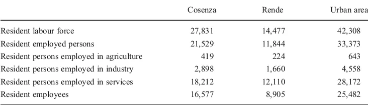
Persons employed in business activities 7,262 3,794 11,056 Persons employed in other private services 6,074 2,844 8,918 Persons employed in public services 13,302 3,300 16,602 Table 2 Resident employment
data Cosenza Rende Urban area
Resident labour force 27,831 14,477 42,308
Resident employed persons 21,529 11,844 33,373
Resident persons employed in agriculture 419 224 643 Resident persons employed in industry 2,898 1,660 4,558 Resident persons employed in services 18,212 12,110 28,172
Although the identified interaction patterns do not necessar-ily lead to rules that can be applied to different geographic
areas, the results of explanatory analysis provide useful information for transportation modelers to re-evaluate the
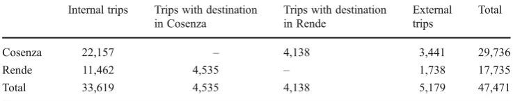
Fig. 3 Daily trips for works and study purposes with the urban area destination Table 4 Daily trips for work
and study purposes Internal trips Trips with destination in Cosenza
Trips with destination in Rende
External trips
Total
Cosenza 22,157 – 4,138 3,441 29,736
Rende 11,462 4,535 – 1,738 17,735
current model structure and to validate the existing model parameters.
Another application of spatial association is in traffic safety [22]. This paper aims at identifying accident hot spots by means of a local indicator of spatial association (LISA), more in particular Moran’s I. For applications in traffic safety, Moran’s I was adapted because road accidents occur on a network. The authors indicated that an incorrect use of the underlying distribution would lead to false results.
Analysis of the literature showed that the spatial analysis techniques were initially applied to the study of socio-economic and demographic variables. Only more recently, these techniques have been applied in the analysis of urban areas and they are still few appli-cations in the field of transport and mobility. Research-ers in the field of transportation, however, have shown a growing interest in applying these techniques to the analysis of mobility. This is because there is a strong
spatial component in the processes of generation and distribution of trips.
This work arises, therefore, to investigate the presence of spatial autocorrelation in the data on the trips distribution in an urban area.
4 The case study
The case study focuses on the urban area of Cosenza, placed in Calabria Region (South Italy). Cosenza, which is the provincial capital in North Calabria Region, forms a single urban area together with Rende in the northerly direction.
This urban area is the most important centre of attraction for all the towns of the province because it performs some administrative functions and offers different services and job opportunities. Furthermore, Rende is home to the University of Calabria (UniCal). The campus affected mobility charac-teristics of all the urban centre of the province. Nowadays the University represents one of the major centres of attrac-tion of the urban area; over 33,000 students and about 2,800 members of staff attend the campus. Thanks to the univer-sity, Rende has changed considerably in recent decades, such as the construction of new residential areas and new infrastructures.
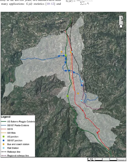
Concerning mobility and transport facilities, the analysed area represents one of the main junctions of the Calabria railways and road system. The motorway A3 Salerno-Reggio Calabria, the SS107 Paola-Crotone state road, and the state road n.19 and n.19bis cross the urban area. Fur-thermore, the urban area is crossing by the railways lines Sibari-Cosenza and Paola-Cosenza, which assure the rail
link between the Tyrrhenian and Ionian rail director. Finally, in the urban area of Cosenza merged the regional railway lines to Catanzaro and Sila, which have a narrow gauge, and are managed by“Ferrovie della Calabria”(Fig.1).
For providing a preliminary characterization of the cities analysed in this work, it is necessary to report some infor-mation about population and economic activities [23].
Concerning population and housing (Table1), more than 70,000 people are resident in the city of Cosenza; on the other hand, the city of Rende has a resident population of about half of Cosenza population. It is necessary to specify that Cosenza and Rende feel the effects of the presence of the University of Calabria; so, in addition to resident people there are other many people (university students) living in the urban area, and especially in the city of Rende.
The population of the urban area is equally spread be-tween males (48 %) and females (52 %). About 68 % of the urban area population belongs to the intermediate class of age (between 15 and 65 years old), which represents the class of persons of working age; about 18 % of people are older than 65 years and about 14 % younger than 15 years. The city of Rende is characterized by a younger population than Cosenza; in fact, only 12 % of people living in Rende is older than 65 years, against a percentage of 20 % for the city of Cosenza; in addition, 15 % of people living in Rende is younger than 15 years, against a percentage of 13 % for the city of Cosenza. This results can be confirmed by calculat-ing the old-age dependency ratio, which is the ratio of the number of elderly persons of an age when they are generally economically inactive (age over 65 in this case) to the number of persons of working age (conventionally 15–65 years old). Specifically, the ratio has a value of 0.26 for the urban area and a value of 0.31 for the city of Cosenza; on the other hand, the value of the old-age dependency ratio for the city of Rende is half of the ratio for Cosenza (0.16).
In the urban area there are about 40,000 families; 70 % of these families lives in Cosenza. A large part of families living in the urban area (about 26 %) have one member; about 23 % of families have two members; more than 40 % are families with three or four components; finally, only 10 % of families have five or more members.
Fig. 5 High/Low clustering output for daily internal trips
Table 5 General G Summary for daily internal trips
General G Summary
Observed General G 0.000348 Expected General G 0.000449
Variance 0.000000
Z Score −3.584739
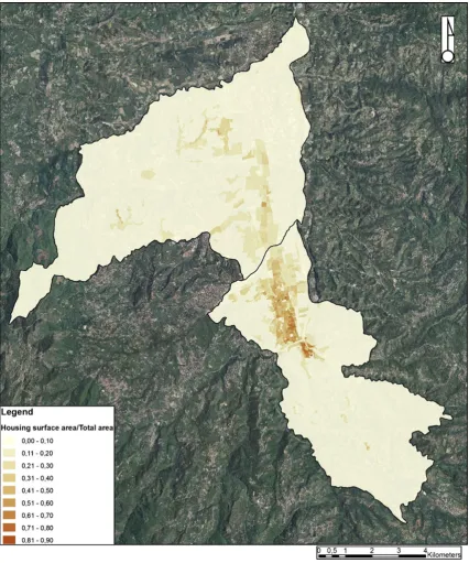
The urban area fills up a surface area of about 82 kmq, and about 55 % of surface area is filled up by the city of Rende. By comparing population and surface area values of the two cities, Rende is larger than Cosenza, but it is less populated. This fact can be confirmed by observing the values of population density, which is the ratio of the pop-ulation of a territory to the total size of the territory; specif-ically, one square kilometre of Cosenza is populated by about 2,000 inhabitants, while about 800 people are on one square kilometre of the area of Rende. The urban area offers about 47,000 housings, of which about 66 % are in the city of Cosenza. By comparing the number of housings and surface area values of the two cities, Rende offers less housing than Cosenza. This fact is confirmed by observing the values of housing density (Fig.2), which is the ratio of the housing of a territory to the total size of the territory. Specifically, 1 km2of Cosenza offers more than 800 hous-ings, while about 350 housings are on 1 km2of the area of Rende.
By observing Fig.2, the old town and the city centre of Cosenza are characterized by the highest values of the ratio of housing surface area to the total surface (between 40 % and 80 %); in the suburb of Cosenza and the town centre of Rende there is a surface area occupied by housing between 10 % and 40 %; finally, in the most marginal areas of Cosenza and Rende the housing density is 10 % at the most. In the urban area there are about 12,000 buildings, of which about 55 % are in the city of Cosenza. Table2shows some data regarding the levels of resident employment and resi-dent employment by sector in the analysed area. Urban area labour force amounts to about 42,000 persons, of which about 66 % of the city of Cosenza, and the remaining
34 % the city of Rende. In the urban area there are about 33,000 resident employed persons, and specifically about 22,000 in Cosenza (65 %).
Obviously, these percentages are correlated to the popu-lation size. In fact, in order to compare the employment data of the two analysed cities and to give more specific infor-mation about the levels of employment, some rates can be calculated.
As an example, the regional employment rate gives an idea about the levels of employment by considering employed persons as a percentage of the population. In this study case, the employment rate is equal to 31 % for the urban area, 29 % for the city of Cosenza, and 34 % for Rende; therefore, Rende has a major number of people employed compared to the total population than Cosenza. Analogously, the regional unemployment rate can be calcu-lated, by considering unemployed persons as a percentage of the economically active population (labour force). The urban area presents an unemployment rate of about 21 %, Cosenza of about 23 %, while Rende has the lowest value, equal to 18 %. By analysing the data about the employment by sector of the studied area, persons employed in the services represent 84 % of the total employed persons, about 14 % of resident persons work in the industry, and only 2 % in the agriculture. Finally, 76 % of employed persons are employees.
Table 3 shows some data regarding the employment in the analysed area. ISTAT provides the data regarding economic activities, through the decennial census of the industrial and service activities [24]. These data show that in the urban area there are predominantly enter-prises operating in the service sector; specifically, there are 9,789 private and public enterprises, with 45,415 persons employed (72 % in Cosenza and 28 % in Rende). The enterprises are generally small, with a staff of 4.4 employed in average. While in Cosenza most of people are employed in the sector of the public services, the enterprises located in Rende refer prevalently to the business activities. About 6 % of the 45,000 persons employed works in the agriculture sector, about 13 % in the industries, and about 81 % in the services.
Fig. 6 High/Low clustering output for daily external trips
Table 6 General G Summary for daily external trips
General G Summary
Observed General G 0.000413 Expected General G 0.000449
Variance 0.000000
Z Score −1.180129
4.1 Daily trips characteristics
Census data of the population [23] also provides the data referred to the daily trips made by people from home to work and study places (commuter trips). The trips are dis-tinguished into trips with destination in the place of resi-dence (internal trips), and trips with destination outside the place of residence (external trips).
However, it is necessary to observe that among the trips from Cosenza some trips have destination in Rende and vice versa. Therefore, these trips are internal trips for the urban area. In order to quantify these, some informa-tion collected by previous surveys are taken into account, and specifically a survey realized on the occasion of the urban traffic plan drafting of Cosenza [25]. The survey, effected in May 2000, was addressed to 649 households (2,014 members) out of 28,499 resident households [26]. From the survey data it follows that there are 32,852 trips per day made (for all purposes) by persons resident in the city with destination in other places, but a relevant part of these (17,924 trips) had their destination in Rende (54.6 %). This percentage can be used for estimating the number of commuter trips with origin in Cosenza and destination in the urban area.
Analogously, from the survey realized in the occasion of the urban traffic plan drafting of Rende [27], a number of 7,293 trips per day made (for all purposes) by persons resident in Rende with destination in other places was esti-mated. Also in this case, a relevant part of the trips (5,272) had their destination in Cosenza (72.3 %). This percentage can be used for estimating the number of commuter trips with origin in Rende and destination in the urban area.
Table4 shows that the percentage of the trips produced by the residents with destination into the urban area is relevant for both for Cosenza and Rende (about 90 % of the total trips).
The trips with destination in Cosenza and those in Rende are been considered as internal trips. As shown in the Fig.3, the internal trips vary between 0 to about 450 for each census parcel. The highest values are concentrated in the urbanized parcels. In Rende these are along the state roads n.19 and n.19bis and in the western region; whereas in Cosenza these are in the northern area. Furthermore, some parcels have numerous daily trips but also a great area. The others census parcels have less internal trips and are localized in the subur-ban areas which have low values of population and housing.
The Fig.4, about the external trips, has a similar config-uration of the Fig. 3 but the values for census parcels are lower. They vary between 0 to about 80 daily trips.
However, it is necessary to point out that census data refer to the trips made for work and study purposes only, but a relevant part of the daily trips is made for other purposes. As an example, by the same survey realized in the occasion of the urban traffic plan drafting of Cosenza it emerges that out of 5,075 home-based trips realized by a sample of residents in Cosenza, 1,924 (38 %) are trips made for work and study purposes, but 3,151 (62 %) area trips realized for other purposes. Therefore, we can retain that 47,471 com-muter trips registered by the census represent only 38 % of the total trips made in a day. By taking into account the complementary percentage (62 %), a realistic value of the daily home-based trips amount to 124,924. This value could be further increased in order to take into account the non home-based amount of trips.
5 Spatial techniques application
Clustering techniques have emerged as a potential approach for analysing complex spatial data in order to determine whether or not inherent geographically based relationships exist. The measures of global and local spatial autocorrela-tion, defined in the Section2, were applied and implemented
Fig. 7 Spatial autocorrelation output for daily internal trips
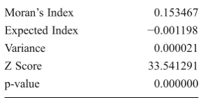
Table 7 Global Moran’s I Summary for daily internal trips
Global Moran’s I Summary
Moran’s Index 0.153467 Expected Index −0.001198
Variance 0.000021
Z Score 33.541291
in a GIS environment for analysing the spatial association of the internal and external daily trips made in the urban area of interest. The computer program ArcGIS contains methods that are most appropriate for understanding broad spatial patterns and trends.
5.1 Global statistics of spatial association
The purpose of the application of global techniques is to understand the spatial distribution of trips among the census parcels in the entire urban area. The tools used for calculat-ing global statistics in ArcGIS areHigh/low Clusteringand Spatial Autocorrelation.
High/Low Clusteringmeasures the degree of clustering for either high values or low values. It calculates the Getis-Ord General G statistics and associated Z score which is a measure of statistical significance. The null hypothesis to reject is“there is no spatial clustering”. When the absolute value of the Z score is large, the null hypothesis can be rejected. The higher (or lower) values of the Z score involve the strong intensity of the clustering. A Z score near zero indicates no apparent clustering within the study area, whereas a positive and a negative Z score indicates cluster-ing of high and low values, respectively. This statistics is very useful to understand the pattern of daily trips in the urban area of Cosenza and Rende.
Regarding the internal trips, the outcomes (Table 5) indicate that the Z score value is negative and high in absolute value; therefore, the null hypothesis can be rejected and there is less than 1 % likelihood that the clustering of low values could be the result of random chance (Fig. 5).
In the case of the application to the external trips, the outcomes (Table6) indicate that the Z score value is nega-tive but his absolute value is lower; therefore, the null hypothesis cannot be rejected.
In the Fig. 6, it is reported the graphic output which shows that even if there is some clustering, the pattern may be due to random chance. Probably, this result is caused by the data set, which for external trips contains low values respect to the internal trips.
Spatial Autocorrelation measures the Global Moran’s I which evaluates whether the analysed pattern is clustered, dispersed, or random. A Moran’s I value near +1.0 indicates clustering whereas a value near −1.0 indicates dispersion. The Global Moran’s I function also calculates a Z score value that indicates whether or not to reject the null hypoth-esis: “there is no spatial clustering”. To determine if the Z score is statistically significant, it is compared to the range of values for a particular confidence level. When the p value is small and the absolute value of the Z score is large enough to fall outside of the desired confidence level, the null hypothesis can be rejected.
Analysing the spatial distribution of the internal trips, it is evident that the Z score value is high and the null hypothesis can be rejected (Table7).
As represented in the Fig. 7, the data are clustered and there is less than 1 % likelihood that the clustered pattern could be the results of random chance.
The results of the spatial autocorrelation applied on the external trips follow the same trend as the previous one, as showed in the Table8.
Therefore, the null hypothesis can be rejected and there is a clustered pattern of the data (Fig.8).
The application of Getis-Ord General G and of Mor-an’s Index I gives similar results from the analysis of internal trips but dissimilar ones for external trips. In fact, for internal trips, the first statistics establishes that there is clustering of low values, and the second one confirms the presence of spatial patterns. Instead, for external trips, the General G statistics says that the distribution of data is random, whereas Moran’s I shows that there is a clustered pattern.
Table 8 Global Moran’s I summary for daily external trips
Global Moran’s I Summary
Moran’s Index 0.163209 Expected Index −0.001198
Variance 0.000021
Z Score 35.724162
p-value 0.000000
5.2 Local statistics of spatial association
The global measures of spatial association refer to the entire area and do not give indications about the clusters are localized. The local statistics of spatial association are useful in detecting places with unusual concentrations of hot spots. The tools of ArcGIS, which are used in this work for applying the local statistics, are Hot Spot Analysis and Cluster and Outlier Analysis.
Hot Spot Analysis calculates the Getis-Ord Gi* sta-tistics for hot spot analysis. The output of the Gi function is a Z score which represents the statistical significance of clustering for a specified distance and must be compared to the range of values for a partic-ular confidence level. A high Z score for a feature indicates its neighbours have high attribute values, and vice versa. A Z score near zero indicates no apparent concentration.
The Getis-OrdGi* statistics applied to internal trips can be displayed graphically by the Z score (Fig.9). The con-centration of“hot”spots (in this case, the concentration of census parcels with high number of daily trips with the destination in the urban area) is represented in red, whereas the concentration of “cold” spots (census parcels with low number of daily internal trips) is in blue. The parcels with high values are localized on the boundary between Cosenza and Rende. In fact, this zone is a
unique urban structure, which has similar characteristics, as said in the Section 4. Instead, the parcels with low values are localized in the old town of Cosenza and in areas with low population.
Similarly, the Getis-OrdGi*statistics applied to external trips (Fig.10) presents concentrations of high or low values in the same zones of the urban areas.
Cluster and Outlier Analysismeasures the Anselin Local Moran’s I and identifies clusters of points with values
similar in magnitude and clusters of points with very het-erogeneous values.
A positive value for I indicates that the feature is sur-rounded by features with similar values. A negative value for I indicates that the feature is surrounded by features with dissimilar values. The tool also provides a Z score value for each observation. A group of adjacent features having high Z scores indicates a cluster of similarly high or low values. A low negative Z score for a feature indicates the feature is surrounded by dissimilar values. Finally, the tool provides a
distinction between a statistically significant (0.05 level) cluster of high values (HH), cluster of low values (LL), outlier in which a high value is surround primarily by low values (HL), and outlier in which a low value is surrounded primarily by high values (LH). The Anselin Local Moran’s I output can be displayed by the visualization of these four patterns of spatial association.
In the Figs. 11 and 12, the patterns are represented for internal and external trips respectively. There is an evident agreement between the two representations. The areas of the
corresponding patterns are localized in the same place, even if their extensions and shapes are different.
Comparing the output ofHot Spot Analysisand Cluster and Outlier Analysis, a certain similarity emerges. In fact, both the statistics give an indication about the localization of the hot and cold spot, which is approximately the same.
The application of the spatial association statistic to com-muting trip data introduced new aspects which merit further consideration, as said in [20]. Moreover, the used measures can improve understanding of the strengths and weaknesses
of the estimated models in terms of a spatial analysis. This understanding can be incorporated into improved and more comprehensive models.
6 Conclusions
have been distinguished into trips with destination in the place of residence (internal trips), and trips with destination outside the place of residence (external trips). Exploratory spatial data analysis was conducted applying both global and local tech-niques of spatial association. The main contribution of the ESDA is to highlight potentially interesting features in the data, and to address the modelling process.
The statistics were elaborated by using GIS, which allows the outcomes to be estimated with automatic proceedings and this aspect facilitates the application of techniques to large data sets. In fact, the application of spatial analysis has obvi-ously become easier with the recent advancements in comput-ing and GIS, which have revolutionized the development of planning support systems to study and simulate the future of travel demand in urban areas.
The results showed that the spatial distribution of trips among the census parcels displays clusters of similar values and there is spatial dependence in the data set. This means that to model the phenomenon is necessary to use spatial regression models because the application of non-spatial regression models can lead to wrong results.
The work presented in this paper is a step towards a wider work regarding the case study of Cosenza-Rende. Future developments will regard the analysis of interaction between land-use and transportation systems, the development of spatial regression models, and it will also comprise the supply transportation system, the localization of dwellings and economic activities, and the territorial features. More-over, further developments will concern the check if the results can be generalized to urban contexts with similar characteristics to that studied.
Open Access This article is distributed under the terms of the Crea-tive Commons Attribution License which permits any use, distribution and reproduction in any medium, provided the original author(s) and source are credited.
References
1. Bertaud A, Stephen M (2003) The spatial distribution of popula-tion in 48 world cities: implicapopula-tions for economies in transipopula-tion, the centre for urban land economic research.http://alainbertaud.com/ AB_Files/Spatia_Distribution_of_Pop_50_Cities.pdf
2. Eboli L, Forciniti C (2010) Spatial analysis and statistics as a tool for analyzing land-use and transportation systems. In: Las Casas G, Pontrandolfi P, Murgante B (eds) Informatica e Pianificazione Urbana e Territoriale. Atti della Sesta Conferenza Nazionale IN-PUT 2010, vol 1. Libria, Melfi, pp 25–36
3. Câmara G, Carvalho MS (2005) A tutorial on spatial analysis of areas.http://edugi.uji.es/Camara/spatial_analysis_areas.pdf
4. Okunuki K (2001) Urban analysis with GIS. GeoJ 52:181–188 5. Scott LM, Janikas MV (2010) Spatial statistics in ArcGIS. In:
Fischer M, Getis A (eds) Handbook of applied spatial analysis: software tools, methods and applications. Springer, Berlin Heidelberg
6. Pàez A, Scott DM (2004) Spatial statistic for urban analysis: a review of techniques with examples. GeoJ 61:53–67
7. Getis A (2007) Reflections on spatial autocorrelation. Reg Sci Urban Econ 37:491–496
8. Anselin L (1988) Spatial econometrics: methods and models. Kluwer, Dordrecht
9. Anselin L, Sridharan S, Gholston S (2007) Using exploratory spatial data analysis to leverage social indicators databases: the discovery of interesting patterns. Soc Indic Res 82:287–309 10. Getis A, Ord JK (1993) The analysis of spatial association by use
of distance statistics. Geogr Anal 25:276–276
11. Ord JK, Getis A (1995) Local spatial autocorrelation statistics: distributional issues and an application. Geogr Anal 27:286–306 12. Ord JK, Getis A (2001) Testing for local spatial autocorrelation in
the presence of global autocorrelation. J Reg Sci 41(3):411–432 13. Anselin L (1995) Local Indicators of Spatial Association-LISA.
Research paper 9331, Regional Research Institute West Virginia University Morgantown
14. Aguiar APD, Câmara G, Escada MIS (2007) Spatial statistical analysis of land-use determinats in the Brazilian Amazonia: ex-ploring intra-regional heterogeneity. Ecol Model 209:169–188 15. Pàez A, Uchida T, Miyamoto K (2001) Spatial association and
heterogeneity issues in land price models. Urb Stud 38(9):1493– 1508
16. Baumont C, Ertur C, Le Gallo J (2004) Spatial analysis of em-ployment and popolation density: the case of the aglomeration of Dijon 1999. Geogr Anal 36:146–176
17. Tse RYC (2002) Estimating neighbourhood effects in house prices: towards a new hedonic model approach. Urb Stud 39:1165–1180 18. Haider M, Miller EJ (2000) Effects of transportation infrastructure
and location on residential real estate values: application of spatial autoregressive techniques. Transp Res Rec 1722:1–8
19. Bolduc D, Laferriere R, Santarossa G (1995) Spatial autoregres-sive error components in travel flow models: an application to aggregate mode choice. In: Anselin L, Florax RJGM (eds) New directions in spatial econometrics. Springer, Berlin, pp 96–108 20. Berglund S, Karlstroëm A (1999) Identifying local spatial
associ-ation in flow data. J Geograph Syst 1:219–236
21. Shaw S, Xin X (2003) Integrated land use and transportation interaction: a temporal GIS exploratory data analysis approach. J Transp Geogr 11:103–115
22. Moons E, Brijs T, Wets G (2009) Improving Moran’s index to identify hot spots in traffic safety. In: Murgante B, Borruso G, Lapucci A (eds) Geocomputation and urban planning. Studies in computational intelligence (SCI) 176. Springer, Berlin Heidelberg, pp 117–132
23. Istituto Nazionale di Statistica (2001) 14° Censimento generale della popolazione e delle abitazioni. Roma
24. Istituto Nazionale di Statistica (2001) 8° Censimento generale dell’industria e dei servizi. Roma
25. Festa DC (2002) Studio per la redazione del Piano Generale del Traffico Urbano del Comune di Cosenza. Dipartimento di Pianifi-cazione Territoriale, Università della Calabria, Rende
26. Istituto Nazionale di Statistica (1991) 13° Censimento generale della popolazione e delle abitazioni. Roma