ABSTRACT
PILGRIM, RYAN ZACHARY. Source Coding Optimization for Distributed Average Consensus. (Under the direction of Dror Baron.)
© Copyright 2017 by Ryan Zachary Pilgrim
Source Coding Optimization for Distributed Average Consensus
by
Ryan Zachary Pilgrim
A thesis submitted to the Graduate Faculty of North Carolina State University
in partial fulfillment of the requirements for the Degree of
Master of Science
Electrical Engineering
Raleigh, North Carolina 2017
APPROVED BY:
David Lalush Michael Daniele
Dror Baron
DEDICATION
BIOGRAPHY
The author was born in Boulder, Colorado in 1991. His childhood was spent in Colorado, Virginia, Mississippi, and North Carolina. After graduating from Hickory High school, he attended the University of North Carolina at Asheville. He then transferred to North Carolina State University to study Biomedical Engineering, graduatingmagna cum laudewith a Bachelor of Science in 2014.
His research interests span statistical signal processing, compressive sensing, and machine learning. He also enjoys programming and embedded systems development. In his spare time, he plays disc golf and the guitar.
ACKNOWLEDGEMENTS
I would like to thank my advisor, Dror Baron, for his patient mentorship and excellent advice. Thanks also to my collaborators Waheed Bajwa and Junan Zhu for their many helpful inputs regarding consensus and the research process. I would furthermore like to acknowledge Yanting Ma for helping to expand the main theorem of the thesis to the more general, variable distortion setting.
TABLE OF CONTENTS
LIST OF TABLES . . . vii
LIST OF FIGURES . . . viii
Chapter 1 INTRODUCTION . . . 1
1.1 Summary of prior art . . . 2
1.1.1 Overview . . . 2
1.1.2 Static, dynamic, and dithered quantization schemes . . . 3
1.1.3 Topology and weight tuning . . . 5
1.1.4 Sequence filtering . . . 6
1.1.5 Wireless considerations . . . 6
1.1.6 Information theoretic approaches . . . 7
1.2 Motivation and contributions . . . 8
1.3 Organization . . . 9
1.4 Notation and acronyms . . . 10
1.4.1 Notation . . . 10
1.4.2 Acronyms . . . 12
Chapter 2 QUANTIZED DISTRIBUTED AVERAGE CONSENSUS . . . 14
2.1 Overview . . . 14
2.2 Mathematical preliminaries . . . 15
2.2.1 Matrix and graph theory concepts . . . 15
2.3 The consensus problem . . . 16
2.3.1 Lossy consensus . . . 18
2.4 Source coding, quantization, and rate-distortion theory . . . 21
2.4.1 Coding and information theory . . . 21
2.4.2 Rate-distortion theory . . . 22
2.4.3 Uniform and nonuniform quantization . . . 26
2.4.4 The quantization noise model and dithering . . . 27
Chapter 3 CODING RATE OPTIMIZATION IN CONSENSUS . . . 30
3.1 Problem formulation . . . 31
3.2 Abstractions for vector-valued data . . . 33
3.3 Assumptions and analytical results . . . 36
3.3.1 Additive noise model . . . 37
3.3.2 Preservation of Gaussian distribution . . . 37
3.3.3 State evolution for vector consensus . . . 39
3.4 Optimization via generalized geometric programming . . . 45
3.4.1 Cost function formulation . . . 47
3.4.2 Basics of generalized geometric programming . . . 50
3.4.3 Proof that the optimization is a GGP . . . 51
3.5.1 Equal-distortion simplification and implementation . . . 54
3.5.2 Efficient search heuristic for fixed-rate quantizers . . . 56
Chapter 4 NUMERICAL RESULTS . . . 58
4.1 Structure of solutions . . . 60
4.1.1 Nonmonotone behavior . . . 62
4.2 Comparison to prior art . . . 70
4.2.1 Implementation details . . . 71
4.2.2 Discussion of comparison results . . . 72
4.2.3 Comparison to predictive coding scheme . . . 75
4.2.4 Comparison to the ProgQ scheme . . . 78
Chapter 5 CONCLUSION . . . 79
LIST OF FIGURES
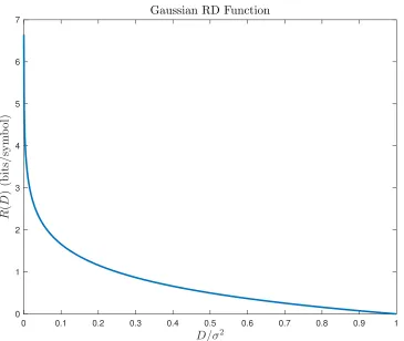
Figure 2.1 The RD functionRpDqof a Gaussian memoryless source. The function is a nonincreasing, convex function of the normalized distortion σD2, where σ2 is the variance of the Gaussian source. The RD pairs above the curve
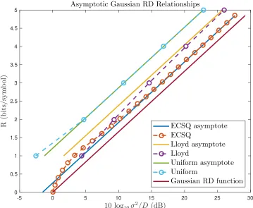
are achievable, while those below the curve are not. . . 23 Figure 2.2 Operational RD relationships of practical quantizers: ECSQ, Lloyd-Max,
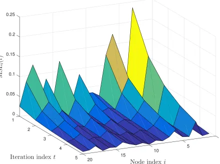
and fixed-rate uniform quantization. Note that all of these approach an asymptote that is a constant offset from the Gaussian RD function as R Ñ 8. The ECSQ performance corresponds to the uniform scalar quantizer with a level at zero. The representation level placement may be suboptimal, but it allows for coding rates below one bit per symbol. This figure was inspired by a similar plot in lecture notes from a TU Berlin source coding course [56]. . . 25 Figure 3.1 Surface showing the evolution of MSEiptqfor the case of lossless
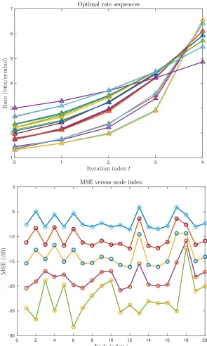
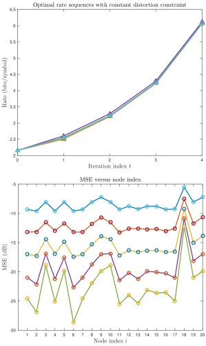
consen-sus. Note that the value of MSEiptq is not equal across all nodes for a particular iteration, and the evolution of MSEiptqis heavily dependent on network topology. Also observe that the MSE decreases monotonically at each node ast Ñ 8. The varianceνiptqevolves in a similar fashion. . 46 Figure 4.1 Optimal rates and MSE sequences from the solution of (3.38) (T “ 5,
ρc “0.35,σx2“1,σn2 “0.5,m“20).Top:Optimal rate sequences for the
variable-distortion optimization problem. The rates are plotted against iteration indices, and each line represents the rates used by a different sensor.Bottom:MSE sequence corresponding to the above rate sequence. The MSE values are plotted against node indices, and each line represents a different iteration. In this case, the MSE values decrease monotonically for all nodes. The lines represent values predicted by the state evolution equations (3.23)–(3.26), and the overlaid circles represent the simulated values. . . 59 Figure 4.2 Optimal rates and MSE sequences from the solution of (3.39) (T “ 5,
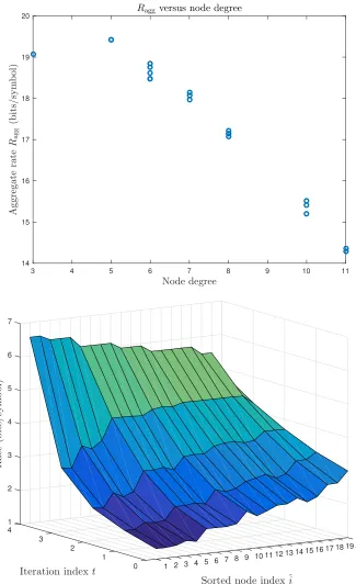
Figure 4.3 Influence of connectivity on the optimal rates from the solution of (3.39) (T“5,ρc “0.35,σx2 “1,σn2“0.5,m“20).Top:Scatter plot of aggregate rate used at each node versus node degree.Bottom: Surface of optimal rate sequences at each node, where the node indices are sorted by node degree in decreasing order. . . 63 Figure 4.4 Nonmonotone optimal rate sequences for the low-SNR, low-MSE setting
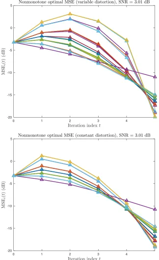
(T “ 5, ρc “ 0.35, σx2 “ 1, σn2 “ 20, m “ 20). Each line corresponds to the rate sequence used by a different node.Top: Variable-distortion optimization (3.38) result.Bottom:Constant-distortion optimization (3.39) result. . . 64 Figure 4.5 Nonmonotone MSE sequences. Each line corresponds to the MSE
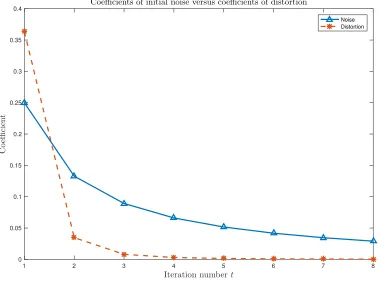
se-quence of a different node (T “ 5, ρc “ 0.35, σx2 “ 1, σn2 “ 0.5). Top: MSE evolution for the variable-distortion problem (3.38).Bottom: MSE evolution for the constant-distortion problem (3.39). . . 66 Figure 4.6 Coefficients of the noise variance σn2 (solid blue curve) and distortion
Dp0q (dashed red curve) in the equation for the MSE (3.31) when the states are initialized as a Gaussian random vector corrupted by AWGN (ρc“0.35,m“20). . . 69 Figure 4.7 RD trade-off curves for the proposed schemes versus order-one predictive
coding [21]. All schemes were simulated for random geometric graphs on a unit torus with connectivity radiusρc“0.35.Top: number of iterations
T“5.Bottom: number of iterations T“7. . . 73 Figure 4.8 RD trade-off curves for the proposed schemes versus order-one predictive
coding [21]. All schemes were simulated for random geometric graphs on a unit torus with connectivity radiusρc“0.45.Top: number of iterations
T“5.Bottom: number of iterations T“7. . . 74 Figure 4.9 RD trade-off curves for the proposed schemes versus ProgQ [20]. All
schemes were simulated for random geometric graphs on a unit torus with connectivity radius ρc “ 0.35. Top: number of iterations T “ 5.
Bottom: number of iterationsT“7. . . 76 Figure 4.10 RD trade-off curves for the proposed schemes versus ProgQ [20]. All
schemes were simulated for random geometric graphs on a unit torus with connectivity radius ρc “ 0.45. Top: number of iterations T “ 5.
CHAPTER
1
INTRODUCTION
The wide availability of wireless sensors and large data sets in recent years has provided significant motivation for the development of distributed computing methods. Large sensor networks and big, distributed data sets pose a number of unique optimization opportuni-ties, including energy management in battery-powered sensor networks [1, 2] and run time reduction in cloud computing applications [3].
optimization, filtering, and environmental monitoring [7]. Consensus algorithms have also found applications in computer vision [8], where they can be used for null-space and least-squares estimation, distributed singular value decomposition, principal components and generalized principal components analyses, point triangulation, and linear pose estimation. Furthermore, consensus algorithms have recently found application in distributed eigenvector estimation and dictionary learning [9].
Although it has a wide variety of engineering applications, consensus originated as a model of social interaction in the management science and statistics communities [10] during the 1960s, according to Olfati-Saber et al. [6]. Its application to the problem of distributed networked computation was first studied by Borkar and Varaiya [11] and Tsitsiklis [12, 13], where it was applied to distributed estimation, optimization, and decision making. Much of the early work on consensus assumed that the nodes could communicate real-valued data to one another [14]. In realistic scenarios, the nodes must communicate within bandwidth and energy constraints, which can have a significant impact on the convergence of distributed averaging algorithms. Although many papers have been published on quantized consensus in recent years [4, 7, 14–28], a large portion consider trade-offs among run time, communication load, and final accuracy in ways that do not take advantage of the tools of constrained optimization. This work attempts to take a more structured approach to the reduction of communication in consensus than past efforts by considering rate-distortion (RD) theory [29, 30] and convex optimization techniques [31].
1.1
Summary of prior art
1.1.1 Overview
quan-tization strategies using both static and dynamic quanquan-tization schemes. Because the classic linear-update consensus algorithms suffer from divergence in the presence of quantized or noisy exchanges [32], many of these works focus on proposing new algorithms and proving their asymptotic convergence properties. A variety of methods has been employed to sidestep the many issues quantization poses, including adapting the quantization range, tuning the weight link sequence, using dithering or randomized quantization, and filtering the past and present state values. This section provides a survey of these works before introducing and distinguishing our approach.
1.1.2 Static, dynamic, and dithered quantization schemes
Early publications on the topic, such as the work of Xiao et al.[32], show that introducing perturbations of constant variance (such as quantization error) into the traditional consensus state update prevents convergence due to the limited precision of the quantizer. Similar convergence issues preclude convergence when the quantization range is held constant [14]. Chamieet al.[16], like Frascaet al.[14], considered the case of nonadaptive, deterministically quantized consensus, and they showed that in finite time, consensus is achieved in the sense that the network state converges to one of the quantization levels.
for a wide class of distributed averaging algorithms.
Due to the difficulties associated with quantization error, many works address the incorpo-ration of dynamic encoding/decoding strategies into consensus protocols. However, many of these schemes do not explicitly consider the RD trade-off and offer certain heuristics to optimize communication performance within their proposed frameworks.
Carliet al.[15, 17] assessed the performance of a “zoom-in, zoom-out” strategy originally studied in the context of quantized feedback control system stabilization. In this scheme, the quantization range grows in the case of saturation and shrinks otherwise. The authors demon-strated convergence for certain topologies, numbers of quantizer levels, and initial quantizer range values. Interestingly, they showed that under certain circumstances, convergence speed can be faster than in the case of ideal, unquantized transmission.
Similarly to Carliet al.[15, 17], Regoet al.[33] proposed an algorithm with progressively shrinking quantization range and derived conditions on the design parameters to guarantee bounded steady-state error. To demonstrate the efficacy of their approach, they simulated a vehicle formation control problem.
algorithm in the limit of many iterations. Both of these works assume a constant coding rate throughout all iterations and rely on differential encoding/decoding to achieve convergence. Yildiz and Scaglione [21, 22, 36], unlike other authors, explicitly considered the RD trade-off to achieve an asymptotic MSE value in consensus with Gaussian states. They proposed schemes based on differential [22], predictive, and Wyner-Ziv coding [21, 36]. In Yildiz and Scaglione [21], the authors exploited the correlation of the current network state with that of previous iterations, and showed that bounded steady-state error is possible under their schemes using shrinking coding rates. Modeling the quantization error as an additive noise, they also provided a necessary and sufficient condition on the variance of the quantization error to ensure convergence. The main focus of the work [21] is to show that convergence can be achieved using asymptotically decreasing coding rates under predictive and Wyner-Ziv coding schemes. In [22], Yildiz and Scaglione considered a simpler case of differential coding and showed similar results for this approach. Yildiz and Scaglione [22] also imposed a parametric form on the distortion sequence and examined the effect of varying the convergence rate on the aggregate coding rate required to achieve a target asymptotic MSE.
1.1.3 Topology and weight tuning
smallest steady-state error can be found via convex optimization.
Mosquera et al.[23] considered a greedy approach to updating the weight sequence by minimizing the minimum MSE (MMSE) of the estimates at each node during each iteration and proposed a modified scheme that only requires statistical knowledge about the topology. The modified scheme approximates a random geometric network by a regular graph, for which each node has the same number of neighbors.
1.1.4 Sequence filtering
To suppress the perturbations resulting from quantization, some authors have considered the possibility of using the history of past state values. Zhu et al. [26, 38] considered the problem of distributed parameter estimation with quantization error, proposed a scheme to reduce randomness using a moving average, and bounded its almost sure performance. Similarly, Thanouet al.[39] considered the problem of quantized distributed averaging and demonstrated a technique to find the optimal polynomial filter coefficients to minimize the effect of quantization error. Fang and Li [40] developed a sequence averaging approach with convergence properties that improved over Frasca et al. [14]. In contrast to Zhu et al. and Thanouet al., Fang and Li only computed the average in the final iteration. These approaches both reduce the randomness introduced by quantization and accelerate the convergence of consensus algorithms.
1.1.5 Wireless considerations
Huang and Hua [28] designed an energy planning algorithm for progressive estimation and consensus in multihop wireless sensor networks (WSNs). They formulated energy models based on assumptions on the wireless channels, and proposed energy optimization approaches for both types of estimation in the presence of quantization. However, Huang and Hua [28] only considered the simple fixed-rate uniform quantizer and did not allow the coding rate to vary over the iterations or nodes in their analysis of consensus.
1.1.6 Information theoretic approaches
Although much of the literature considers the design of specific protocols for consensus averaging, a handful of works have explored the fundamental RD limits in the distributed computation problem. Two of these derive bounds on computation time using information theoretic inequalities [41, 42], but they do not consider RD theory [29, 30] in their analyses. Recently, Su and El Gamal [43] considered the problem of computing the RD function for distributed average consensus using peer-to-peer communication protocols. The authors derived a closed form for the RD function for a two-node network, and derived upper and lower bounds on the RD function for weighted-sum and gossip-based protocols in arbitrary networks. However, the authors restricted their attention to a class of protocols that uses communication between node pairs and assumes time-invariant normalized distortion. The analysis of this thesis, by contrast, assumes communication among more than one agent at each time step (corresponding to broadcast, rather than peer-to-peer, protocols), greater flexibility in the selection of edge weights, and time-varying distortions. Furthermore, Su and El Gamal did not present results on the tightness of their weighted-sum or gossip bounds, nor did they demonstrate the achievability of these bounds except in the case of a large star network with a centralized protocol.
communicating its result to the next node in the path. The second scenario is that of consensus, in which each node forms an estimate of the desired quantity. Although Yang et al. [44] provided bounds on the RD relationship for consensus in tree networks and proved the achievability of the derived bounds, their analysis is limited to the setting where the network is tree-structured. Often it is beneficial to consider more flexible topologies, such as random geometric graphs [45], which have been used to model WSNs [46]. In general, random geometric graphs and their real-world WSN counterparts have loops.
1.2
Motivation and contributions
numerical experiments.
The advantages of our approach are (i) ignorance about the parametric form of the distortions, which allows greater flexibility in the selection of the optimal rates, (ii) support for different rates at each node and iteration of the algorithm, and (iii) optimization with respect to exact MSE quantities for finite iteration count.
Point (i) distinguishes our approach from Yildiz and Scaglione [22], who restricted their study to optimal distortion sequences that formed convergent series. Point (ii) contrasts this thesis with the work of Huang and Hua [28] and Thanouet al.[20], who required the use of a fixed-rate uniform quantizer with a rate that was constant over both nodes of the network and iterations of the algorithm. Point (iii) differentiates this thesis from both Huang and Hua [28] and Yildiz and Scaglione [21, 22]; Huang and Hua [28] optimized with respect to a bound on the MSE, and Yildiz and Scaglione [21, 22] considered theasymptoticMSE as the number of iterations goes to infinity.
1.3
Organization
1.4
Notation and acronyms
1.4.1 Notation
In this thesis, uppercase bold letters (e.g.,A) will be used to denote matrices, and lowercase bold letters (e.g.,x) will be used to denote vectors. Vectors that vary with time are assigned a time index, so that a time-varyingx becomesxptq. Scalars that vary with time are denoted
similarly (e.g.,xptq). A superscript on a square matrix (e.g.,Ak, APRnˆn,ka positive integer) denotes raising that matrix to thekth power (i.e, multiplying that matrix by itselfk´1 times). Random variables (RVs) are not distinguished by notation to avoid confusing vectors and matrices.
The following list enumerates frequently used notation and variables and their associated meanings. The meaning of the following notation may not be clear until later, and it is provided here for the reader’s reference.
• t¨uJ: transpose
• Qp¨q: quantization function
• I: identity matrix
• 0: the matrix or vector of all zeros • 1: vector of all ones
• R: real numbers • Z: integers
• Zě0: nonnegative integers
• Zą0: positive integers
• N pµ,Σq: multivariate Gaussian distribution with meanµ and covarianceΣ • k¨kp:`p norm
• G: undirected graph
• V: vertex (node) set of a graph • E: edge set of a graph
• Ni: neighborhood of nodei • X,Y: finite subsets ofR
• Hpxq: entropy of the random variablex
• Ipx;yq: mutual information between the random variables xandy • ppxq: probability mass function (PMF) of the discrete random variablex
• fpxq: probability distribution function (pdf) of the continuous random variablex • Φxpωq: characteristic function of the random variable x
• Upa,bq: uniform distribution with minimuma and maximumb
• r¨si:ithcomponent of a vector • r¨sij:pi,jqthcomponent of a matrix
• µxptq: mean of the random vectorxptq
• Σxptq: covariance matrix of the random vectorxptq
1.4.2 Acronyms
Here we define a number of acronyms that will be used throughout the work. • AWGN: additive white Gaussian noise
• CLT: central limit theorem
• ECSQ: entropy-coded scalar (uniform) quantization/quantizer • GP: geometric program/programming
• GGP: generalized geometric program/programming • i.i.d.: independent and identically distributed
• LMMSE: linear minimum mean square error • LSE: log-sum-exponential or log-sum-exp • MMSE: minimum mean square error • MSE: mean square error
• PMF: probability mass function • pdf: probability density function • RD: rate-distortion
• RV: random variable • RVec: random vector
CHAPTER
2
QUANTIZED DISTRIBUTED AVERAGE CONSENSUS
This chapter presents much of the background required to understand consensus and source coding. The results presented here are not original, and they are presented to make the thesis self-contained. Our original results appear in Chapters 3 and 4.
2.1
Overview
One of the many attractive features of the variety of distributed average consensus algorithms explored in this thesis is its linearity. At each iteration, every node takes a weighted average of incoming messages from its neighbors, and in the absence of quantization errors, the performance is elegantly described using concepts from spectral graph theory [6, 37].
Although dithering and high-resolution assumptions greatly simplify the analysis of distributed average consensus, close attention must be paid to the design of the state update. If quantization errors are introduced into the lossless algorithm, then the network state will not converge to the true sample average [21, 32]. However, by making a simple modification to the state update, Frascaet al.[14] guaranteed convergence to within one quantization bin. In contrast, prior efforts [21, 22, 32] could only guarantee bounded asymptotic mean square error (MSE) due to the drift from the sample average in the presence of quantization error.
In this chapter, we explore the fundamentals of distributed average consensus, algorithmic modifications to account for quantization effects, rate-distortion (RD) theory, and the basics of the additive noise model for quantization error.
2.2
Mathematical preliminaries
Before introducing the consensus problem, it is first necessary to introduce a number of mathematical concepts related to linear algebra and graph theory.
2.2.1 Matrix and graph theory concepts
To represent the network of interest, it is necessary to model the nodes, which represent the computing elements or agents. These can be wireless sensors [7, 28], servers [9], cameras [8], or robots [6]. We assume that each node can only communicate with a subset of the other nodes of the network, so it is also necessary to model the presence or absence of communication links between them, which can be wireless channels or wired connections. These relationships are modeled by a graph [37].
the simplest representations of the graph is a pair of sets,
G “ tV,Eu, (2.1)
where the graphG is comprised of a set of vertices (nodes)V and a set of edgesE between pairs of vertices [54, Sec. 1.2]. Because the communication links are bidirectional, each edge
ti,ju PE is represented as an unordered pair of verticesiandj[37].
2.3
The consensus problem
In the simplest case of the consensus problem, each nodeiP t1, . . . ,mu has an initial scalar quantity
zip0q PR, (2.2)
and the goal is to have all nodes of the network agree upon the sample mean of these quantities by iteratively exchanging messages with their neighbors [37]. The quantitiesziptq will be referred to as “states,” which in this thesis are assumed to be real-valued scalar random variables (RVs) with known distribution. More formally, let the (discrete) iteration index be a nonnegative integer,1t PZě0. Att“0, the statestziptqumi“1are the initial values to be averaged
by the consensus algorithm. Fort ě1, the stateziptqrepresents the estimate of the sample average
s
z :“ 1 m
m
ÿ
i“1
zip0q
at nodei. The objective of consensus is for the stateziptqto eventually equal the sample mean of the initial states [37]. Mathematically, this is expressed as limtÑ8ziptq “zs,@iP t1, . . . ,mu[37].
1We denote the positive subset of a setSbyS
ą0. The nonnegative subset is similarly denotedSě0. The integers
We leave the discussion of vector-valued states for the following chapter. In this thesis, we restrict our attention to deterministic, synchronous-update consensus algorithms. We assume the following: (i) the communication link topology of the network is fixed and does not change with time, (ii) at each iteration, every node of the network exchanges messages with only its neighbors, and (iii) the communication channels between nodes are noiseless.
Given the above assumptions on communication, one of the most popular algorithms for consensus relies on linear updates [6, 37]. Each node is assigned an indexiP t1, . . . ,mu. Let ziptq denote the state of the ith node at iterationt. Each node updates its state by taking a weighted sum of its own state with those of its neighbors [37],
zipt`1q “wiiziptq `
ÿ
jPNi
wijzjptq, (2.3)
where wiją0@i,j,
řm
k“1wik“1, andNi denotes the neighborhood of nodei,
Ni :“ tj| ti,ju PEu.
The degree of node iis defined as
degi:“ |Ni|,
where | ¨ | represents set cardinality. By this definition, degiis the number of neighbors of nodei. The weightswij are designed such that [37]
lim
tÑ8ziptq “sz.
If the state of each node of the network is collected in a vector
and the averaging weightswij are collected in a matrix,
rWsij :“wij, (2.5)
then the above update equation (2.3) can be written in matrix-vector form as [37]
zpt`1q “Wzptq. (2.6)
The design of the weight matrix W that yields the fastest convergence is a well studied problem; the interested reader is referred to Xiao and Boyd [37]. To converge asymptotically, that is,
lim tÑ8zptq “
1 m11
Jz
p0q “sz1,
the weight matrix must be doubly stochastic, ř
iwij “
ř
jwij “ 1, and the modulus of its largest eigenvalue must be less than unity [37].
2.3.1 Lossy consensus
By introducing quantization error into the internode messages, the simple linear iteration above (2.6) is not guaranteed to converge. Instead, we use the modified iteration proposed by Frasca et al. [14], which allows the sample average to be preserved in the presence of quantization error.
we use the update proposed by Frascaet al.[14], which is
zipt`1q “ziptq ` m
ÿ
j“1
wij
`
Qjpzjptqq ´Qipziptqq
˘
, (2.7)
or in matrix-vector form,
zpt`1q “zptq ` pW´IqQpzptqq. (2.8)
The key advantage of this update is that the average m1 řm
i“1ziptqof the statesziptqis preserved at each stept, despite the presence of quantization error [14]. Defining the quantization error
eptq:“Qpzptqq ´zptq, (2.9)
the preservation of the sample mean can be seen by rewriting (2.8) as
zpt`1q “zptq ` pW´Iq pzptq `eptqq
“Wzptq ` pW´Iqeptq, (2.10)
and then taking the sample mean [14],
1 m1
Jz
pt`1q “ 1 m1
JWz ptq ` 1
m1 J
pW´Iqeptq.
Because W is doubly stochastic,1JW
“1J, and the mean at iterationt
mean at iterationt [14]:
1 m
m
ÿ
i“1
zipt`1q “ 1 m1
Jz pt`1q
“ 1 m1
J
Wzptq ` 1 m1
J
pW´Iqeptq “ 1
m1 Jz
ptq ` 1 m
´
1J ´1J¯
looooomooooon
“0
eptq
“ 1 m1
Jz
ptq “ 1 m
m
ÿ
i“1
ziptq. (2.11)
In this thesis, we model the quantization erroreptqas additive noise.
Note that the target state of consensus, termed theaverage consensus state, can be written,
z˚ : “sz1,
which means thatziptq “sz,@iP t1, . . . ,mu. We also define theaverage consensus operator 1
m11J, so that [37]
1 m11
Jz
p0q “z˚.
Defining the error from the true sample mean,
eptq:“zptq ´z˚ “zptq ´ 1
m11 Jz
p0q, (2.12)
and noting that the average is preserved over the iterations, (i.e., m11Jz
ptq “ m11Jz
pt`1q), the erroreptqcan be expressed as [14]
eptq “
ˆ
I´ 1 m11
J
˙
2.4
Source coding, quantization, and rate-distortion theory
Digital systems rely on the ability to transmit and store information. To perform these tasks reliably, the information takes the form of strings of symbols belonging to some finite alphabet [30]. As a cornerstone of digital communication and storage, coding has been studied quite extensively. In this section, we present some of the fundamental coding and quantization concepts required to understand this thesis.
2.4.1 Coding and information theory
Understanding data compression requires a few concepts from information theory [30], initially developed by Shannon in the 1940s [55]. This theory offers insight into the fundamental limiting performance of communication and compression systems [30]. In this subsection, we focus on the case where the source to be encoded,xPRn, is mapped to a point ˆxin some finite setXn by the quantization operatorQp¨q.
Theentropyof a scalar RVxPX with probability mass function (PMF)ppxqis given by [30]
Hpxq:“ ´
ÿ
xPX
ppxqlog2ppxq.
Intuitively, the entropy of an RV is a measure of its uncertainty or information content [30]. LetxPRnrepresent a long sequencex, the entries of which are independent and identically distributed (i.i.d.) according to the probability mass function (PMF) ppxq. ThennHpxqis the minimum expected binary sequence length required to describex without error [30]. That is, if we wish to describe the sequencexby a string of binary digits ˜xP t0, 1uM, then a code exists such that the original sequencexcan be noiselessly reconstructed from ˜xprovided that
RVs. Letxandybe RVs with joint PMFppx,yqand marginal PMFsppxqand ppyq, respectively.2 Then the mutual informationbetween xPX andyPY is given by [30]
Ipx;yq:“ ÿ
xPX
ÿ
yPY
ppx,yqlog2 ppx,yq ppxqppyq.
The utility of these information-theoretic quantities will become apparent during the discussion of RD theory.
2.4.2 Rate-distortion theory
The previous discussion of coding considered only RVs that take on a finite set of values. If we wish to digitally communicate or store a continuous source, it must first be quantized [35, Ch. 1]. The two most basic elements of a quantizer are a set ofrepresentation levels, which are used to approximate the unquantized signal, and a set ofdecision thresholds, which determine the mapping from the input set to the output set [35, pp. 133–135]. If we imagine the source data as an RV x P Rn, then the quantizer Q : Rn Ñ Xn maps x to one of finitely many representations ˆxPXn[35]. For real-valued sources, quantizers necessarily introduce a certain expected distortion D into their representation of the input signal [35, pp. 144–145]. This distortion can be quantified using a number of metrics, but for the purpose of this thesis, we use the square error metric [35]
dpx, ˆxq “kx´xˆk22,
so that the expected distortion per entry orper letteris given byD“ 1nE“kx´xˆk22‰. In general,
using a higher coding rate R results in a lower distortion D, with the drawback of greater communication load. RD theory [29, 30] quantifies the best possible trade-off between coding rate and distortion using the tools of information theory.
0 0.1 0.2 0.3 0.4 0.5 0.6 0.7 0.8 0.9 1
D/σ2 0
1 2 3 4 5 6 7
R
(
D
)
(b
it
s/s
y
m
b
ol
)
Gaussian RD Function
Assume that we wish to encode a memoryless source, which is represented by the random vector (RVec) x P Rn, xi i.i.d. „ fpxiq,@i P t1, . . . ,nu. For the remainder of this subsection, we drop the indices on xi due to the assumption that all entries of xare i.i.d. The minimum coding rate Rrequired to produce an expected distortion less than or equal to a particular valueDis given by the so-called RD functionRpDq[29, 30],
RpDq:“ min
ppxˆ|xq:Erdpx, ˆxqsďDIpx; ˆxq.
In words, the RD function is the minimum of the mutual information over all possible “test channels” ppxˆ|xq, subject to the constraint that the expected distortion per entryErdpx, ˆxqsis less than a specified valueD [30]. Operationally, the RD function is the minimum number of bits per symbol required to describe a long i.i.d. source within the prescribed distortion D[30]. The computation of a closed form forRpDqis difficult in general; however,RpDqcan be computed numerically [57–59]. When a particular quantizer is used, it will often have an RD trade-off curve that differs fromRpDq, which is a bound on the best possible performance [35]. In this thesis, we term such a trade-off curve for a particular practical quantizer anoperational RD relationshipto avoid ambiguity. An example RD function for the Gaussian case is given in Figure 2.1. Figure 2.2 shows the performance of practical quantizers compared to both the Gaussian RD function and their respective operational RD relationships. Note that the signal-to-distortion ratio (SDR),
SDR :“ varpxq
D ,
-5 0 5 10 15 20 25 30 10 log10σ2/D(dB)
0 0.5 1 1.5 2 2.5 3 3.5 4 4.5 5
R
(b
it
s/s
y
m
b
ol
)
Asymptotic Gaussian RD Relationships
ECSQ asymptote ECSQ
Lloyd asymptote Lloyd
Uniform asymptote Uniform
Gaussian RD function
2.4.3 Uniform and nonuniform quantization
From a conceptual standpoint, one of the simplest quantizers is the familiar uniform scalar quantizer, for which both the representation levels and the decision thresholds are uniformly spaced [35]. For a given input x, a uniform scalar quantizer simply rounds each xi to the representation level ˆxi nearest to xi [35]. This type of quantizer is frequently encountered in analog-to-digital conversion and various digital signal processing systems. Despite its simplicity, this quantizer performs surprisingly well in certain scenarios.
Consider a source xPRn that is not uniformly distributed. For a uniform scalar quantizer, each representation level ˆxi will occur with different probability. In this case, we can choose the representation levels based on the input statistics to obtain a low-distortion quantizer [35]. This idea was explored by Lloyd [60] and Max [61], who developed necessary and sufficient conditions for quantizer optimality, given a fixed number of representation levels and a certain source distribution. Lloyd and Max also developed algorithms for achieving an efficient quantizer by iteratively updating the thresholds and representation levels [35]. Because the quantizer is optimized for a particular number of representation levels, Lloyd-Max quantizers are useful for fixed-length codes, where the encoded sequence ˜xP t0, 1unR. However, more sophisticated coding techniques, such as Huffman coding [62], can be used to approach the previously discussed entropy lower bound on code length if the lengthMof the binary code sequence ˜xP t0, 1uM is allowed to vary with the input [35].
approach asymptotes that are a constant offset from theRpDqfunction in the limitRÑ 8[35]. The asymptotic offset is illustrated in Figure 2.2.
The curious reader might wonder how the optimal quantizer can differ from the bound if the bound is, in fact, achievable. Better performance can be achieved by quantizing long sequences of the source jointly. Interestingly, this is advantageous even if the source symbols are independent [30]. This technique is termedvector quantization (VQ)[35].
Because of the performance improvement associated with VQ, we also consider the multidimensional extension of the scalar quantizer, which is the lattice quantizer [35]. These quantizers approach the RD lower bound for memoryless Gaussian sources [66] as the block dimension approaches infinity, while also permitting the application of dithering, which we will discuss in the following sections.
2.4.4 The quantization noise model and dithering
One of the nicest properties of distributed averaging algorithms is their linearity [14]. At each iteration, a weighted sum of the incoming messages is computed at each node [6, 37]. This allows us to exploit the properties of linear operators, and, for Gaussian-distributed initial states, we can describe the entire network state statistics using linear algebra [21]. However, quantization is inherently nonlinear, which complicates the analysis [14]. Luckily, under certain conditions, the quantization error can be modeled as an additive noise that is uncorrelated with the source [52, 53, 67].
In undithered quantization systems, the conditions for i.i.d. uniform quantization error are rather restrictive [53]. In most cases, these conditions are not met exactly, and the additive quantization noise model is used as an approximation to the true behavior that simplifies system design [52]. In general, the approximation resulting from assuming the additive quantization noise model improves with higher coding rates [52, Sec. 9.5].
More precisely, letxPRn represent a vector to be quantized. The quantizerQp¨q:RÑXn
error,
e:“xˆ´x,
the quantization noise model can, for our purposes, be summarized by the following three relationships: (i) the quantization error is zero-mean,
Eres “0,
(ii) the quantization error is uncorrelated with the source,
E”exJı “0,
and (iii) the quantization error entriesresi andresj,i‰j, are uncorrelated,
E”eeJ
ı
“ b
2
12I,
where bis the quantizer bin size andI is the identity matrix [52].
In situations that discourage or forbid the use of high rates, a technique calleddithering can be used to cause the quantization error to be uncorrelated with the source [53]. Dithering is the process of intentionally adding noise to the source signal x P Rn to randomize the quantization error, which is otherwise a deterministic function of the quantizer input [53]. If the i.i.d. noisewP Rn satisfies certain technical conditions, and the receiver subtracts w from the reconstructed signalQpxq, then the previously discussed additive quantization noise model becomes exact in the sense that [53]
and
E”pQpx`wq ´ px`wqqpQpx`wq ´ px`wqqJ
ı
“ b
2
12I.
Therefore, the quantization error can be modeled as an additive white noise with variance b2
12, which is uncorrelated with the input signalx[53]. The subtraction of the dither can be
achieved in practice using a particular pseudorandom number generator with a seed that is known to both the transmitter and receiver.
CHAPTER
3
CODING RATE OPTIMIZATION IN CONSENSUS
Depending on the system of interest, communication may be more or less expensive relative to run time [47]. For instance, consider two extremes of distributed computing: wireless sensor networks (WSNs) [1, 2] and multiserver networks [3]. WSNs have limited battery life and must communicate over wireless channels, which consumes a large amount of power. In many WSN applications, communication is expensive due to the low-power constraints at each node [47]. By contrast, multiserver networks, such as those used in cloud services [3] have less stringent communication requirements, and the run time is more significant to the user [47]. In these networks, the nodes communicate over wired connections and do not have battery power constraints. To produce an optimization that is useful in diverse distributed settings, then, we pursue a general and simple approach that models the relative costs of communication and computation.
generalized geometric program (GGP).
The first contribution is minor, since similar approaches to computing the network state statistics were derived in Yildiz and Scaglione [21] and Huang and Hua [28]; however, our derivation allows for the explicit computation of MSE expressions in closed form using the iteration (2.7) introduced in Frascaet al.[14]. Yildiz and Scaglione [21] only derived a closed form for the asymptotic MSE as the iteration indext Ñ 8, and Huang and Hua optimized with respect to an MSE bound. Our analysis allows an exact optimization to be performed in the finite-iteration (total iterationsTă 8) case.
The second contribution allows the problem to be formulated in a well-understood frame-work. The GGP model can be converted into convex form and efficiently solved using common numerical techniques [31]. Furthermore, due to the convexity of the equivalent transformed optimization problem, the solver is guaranteed to find the globally optimal solution [31]. In addition to the GGP model, we present a heuristic approach for optimization of fixed-rate source coding schemes. This model reduces the size of the optimization problem, which still provides the same solutions as exhaustive search.
3.1
Problem formulation
At every iterationtP t0, . . . ,T´1uof the consensus process, each nodeiP t1, . . . ,muuses a
coding rate Riptq to encode its state for transmission to the neighboring nodes.1 In general,
Riptqcan vary across both nodes and iterations. In practice, we want to terminate the consensus process after a finite number of iterationsT. We simplify notation by defining thecoding rate vector
We denote the expected distortions per entry incurred by transmitting states using the coding ratesRby thedistortion vector
D:“ rD1p0q, . . . ,Dmp0q, . . . ,D1pT´1q, . . .DmpT´1qsJ. (3.2)
One key quantity we use to determine the cost of running the consensus process is the aggregate coding rate[47, 51]:
Ragg :“
T´1 ÿ
t“0
m
ÿ
i“1
Riptq, (3.3)
which represents the total coding rate used over theTiterations of the consensus algorithm by allmnodes of the network. To address the trade-off between communication and computation, we borrow the following composite cost function from Zhu and coauthors [47–51] that models both communication and run-time costs:
CtotalpR,Tq:“K1Ragg`K2T, (3.4)
whereK1andK2 represent the costs of communication and computation, respectively. Since
the iteration (2.8) consists only of a quantization and a weighted sum at each node, the total run-time cost is modeled as linear in the number of iterations. This cost function can be used to model both battery-powered sensor networks and server networks by varying the relative values ofK1 andK2 [47, 51].
In this chapter, we present minimization strategies of the subcost
CcommpR,Tq:“K1Ragg (3.5)
be found by fixing T and minimizing the communication cost CcommpR,Tq, subject to the
constraint thatRachieves a target mean square error (MSE) value. Repeating this procedure forTP tTmin, . . . ,Tmaxuis equivalent to minimizing overTandRjointly.
To efficiently encode the data stored across the network, it is necessary to understand the evolution of its distribution over time. In general, this is not tractable due to the need to track dependences among source elements and transformations of source densities. Instead, we propose an efficient optimization scheme for entropy-coded uniform scalar quantization (ECSQ) [35] of stationary Gaussian states and rate-distortion-optimal (RD-optimal) vector quantization (VQ) [29, 30] of memoryless Gaussian-distributed initial states.2We also use the resulting strategies to design a coding rate optimization heuristic for a particular dithered fixed-rate uniform quantizer [52, 53], for which the expected distortion is the same regardless of source distribution [53].
In this thesis, we assume that the node-to-node communication is taking place in abroadcast manner [36], which means that the total rate expended by a transmitting node is independent of the size of its neighborhood. This also simplifies the analysis of the introduced distortion, because each neighbor of a particular node will receive the same quantized message.
3.2
Abstractions for vector-valued data
The concepts presented in this section are included for clarity. We will later present simplifica-tions for the case that each node has a stationary Gaussian source. Although not used directly in our optimization model, the mathematics presented in this section is useful for computing the source statistics across the network in a general setting.
jthelement of the stateζiptqas
ζjiptq:“ rζiptqsj. (3.6)
These states are Gaussian random vectors (RVecs) that may be correlated, so thatE
”
ζkiptqζljptq
ı
‰
0 in general.
To model the state of the entire network, we define thenetwork state supervectorζptq PRmL
as follows:
ζptq:“
”
ζ11ptq ¨ ¨ ¨ζ1mptq
ˇ ˇ ˇ ζ
2
1ptq ¨ ¨ ¨ζ2mptq
ˇ ˇ ˇ ¨ ¨ ¨ ˇ ˇ ˇ ζ L
1ptq ¨ ¨ ¨ζmLptq
ıJ
. (3.7)
During consensus, each partition of ζptq in (3.7) is averaged independently (i.e., the vector states are averaged over the network nodes elementwise). To represent this elementwise action, we use thedirect sumoperator for matrices [68]:
n
à
i“1
Ai :“
» — — — — — — — –
A1 0 ¨ ¨ ¨ 0
0 A2 ¨ ¨ ¨ 0
..
. ... . .. ... 0 0 ¨ ¨ ¨ An
fi ffi ffi ffi ffi ffi ffi ffi fl .
Therefore, the operatorÀ
creates a block-diagonal matrix from the matricestAiuni“1. Note that Àn
i“1Ai is shorthand for A1‘A2‘ ¨ ¨ ¨ ‘An. This is an alternative to the Kronecker product notation and the matrix structure introduced by Huang and Hua [28].
Defining the weighted averaging matrix ΩPRmLˆmL:
Ω :“
L
à
l“1
W (3.8)
equivalent to (2.8) for vector consensus is
ζpt`1q “ζptq ` pΩ´IqQpζptqq, (3.9)
where
Qpζptqq:“
”
Q1pζ11ptqq ¨ ¨ ¨Qmpζ1mptqq
ˇ ˇ ˇ Q1pζ
2
1ptqq ¨ ¨ ¨Qmpζ2mptqq
ˇ ˇ ˇ ¨ ¨ ¨
ˇ ˇ ˇ Q1pζ
L
1ptqq ¨ ¨ ¨QmpζmLptqq
ıJ
.
As in the scalar consensus case, we define the quantization error,
δptq:“Qpζptqq ´ζptq. (3.10)
This is the vector consensus analog to eptq (2.9). Using the preceding definitions, the state update (3.9) can be rewritten as
ζpt`1q “Ωζptq ` pΩ´Iqδptq. (3.11)
The goal of vector consensus is to iteratively drive eachζiptqto the sample mean of the initial
statesζip0q. Definesζ PRL as the sample mean (over nodes) of the initial states,
sζ :“ 1
m
m
ÿ
i“1
ζip0q.
The goal of consensus is thus
lim
tÑ8ζiptq “
sζ, @iP t1, . . . ,mu.
consensus state.This state has the following form:
ζ˚“
« “
s
ζ‰1¨ ¨ ¨“sζ ‰ 1 ˇ ˇ ˇ “ sζ ‰ 2¨ ¨ ¨
“ s
ζ‰2
ˇ ˇ ˇ ¨ ¨ ¨ ˇ ˇ ˇ “ sζ ‰
L¨ ¨ ¨
“ s
ζ‰L
ffJ
.
The vector average consensus operatoris defined as
M:“
L
à
l“1
1 m11
J, (3.12)
so that
Mζp0q “ζ˚.
The state estimation error, which is the error in the current estimate of the true average, is defined as
ηptq:“ζptq ´Mζp0q. (3.13)
Because Mζpt`1q “ Mζptq “ Mζp0q [this follows from (2.11)], the error (3.13) can also be expressed as
ηptq “ pI´Mqζptq.
3.3
Assumptions and analytical results
3.3.1 Additive noise model
Following Frascaet al.[14] and Yildiz and Scaglione [21, 22], we adopt the additive model for quantization noise [52]. This model assumes that the errors introduced by the quantization process are uncorrelated with the quantizer input. A formal statement of the corresponding assumptions is provided.
We assume that the quantization errorδptqis spectrally white:
Assumption 1 The quantization error elementδkiptqcorresponding to ζkiptq(3.6) (i.e., quantization error at the kth element of the ith node at iteration t) is uncorrelated with all other quantization error
elements: if j‰i, l ‰k, orτ‰t,E
”
δikptqδljpτq
ı
“E“δikptq‰E
”
δjlpτq
ı
“0.
We further assume that the quantization error is independent of the source to be quantized: Assumption 2 The quantization errorδptqis orthogonal to the state supervectorζptqwith respect to node index (i.e.,E
”
ζptqδJptq
ı
“0).
These assumptions are well motivated for uniform quantizers with high coding rate [52], or for uniform quantizers using dither at arbitrary rates [53]. In general, probability-density-optimized (pdf-probability-density-optimized) quantizers will have quantization error that is linearly correlated with the input signal (i.e., ErxpQpxq ´xqs “ ´D, where x is a scalar RV to be quantized, Qpxqis the result of quantization, andDis the expected distortion) [35, p. 182, 69]. Although dither for nonuniform quantization is not as well studied as for uniform quantization, the problem of correlated quantization noise may be alleviated by dithering using a compander as shown in a recent paper by Aykol and Rose [70]. For quantizers with nonuniform level spacing, Assumptions 1 and 2 are not rigorously justified, but numerical results are included to assess performance.
3.3.2 Preservation of Gaussian distribution
distribution of the state supervectorζptqwill be Gaussian for alltP t0, . . . ,T´1u.
Lemma 9 Assume the technical conditions of Assumption 1 hold. Further assume that the degree of each node is bounded from below by a monotone increasing function gpmqof the network size m. Then
the state supervectorζptq,tP t0, . . . ,T´1u, will be Gaussian distributed.
Proof:The proof follows from a simple application of the central limit theorem (CLT). At the beginning of iteration zero, the random vectorζp0qis jointly Gaussian by assumption. The state supervector is updated as (3.11),
ζpt`1q “Ωζptq ` pΩ´Iqδptq.
If the elements of ζptq are jointly Gaussian, then the term Ωζptq will also be Gaussian distributed, because it is a linear transformation of jointly Gaussian RVs. As m Ñ 8,
|Ni|ěgpmq Ñ 8,@i. Define the “aggregate quantization error” as
δaggptq:“ pΩ´Iqδptq.
Because the degree of each node degiÑ 8,@iP t1, . . . ,mu, each element“δaggptq ‰
k ofδaggptq is a sum of many independent RVs. By the CLT and our assumption of zero-mean inde-pendent quantization error, δaggptq converges in distribution to Np0,pΩ´IqΣδptqpΩ´Iqq,
whereΣδptq:“E
”
δptqδJptq
ı
is the covariance matrix of the quantization errorδptq. Because both terms of (3.11) are Gaussian distributed, ifζptqis Gaussian, thenζpt`1q will be Gaus-sian. Therefore, by our assumption of initial Gaussian state, the state ζptq will be Gaussian
distributed for allt P t0, . . . ,T´1u.
˝
3.3.3 State evolution for vector consensus
Because the network state supervectorζptq(3.7) is Gaussian for allt, the sufficient statistics of
ζptqare a mean vector and covariance matrix. Likewise, because the errorηptq(3.13) is a linear
transformation ofζptq, it has a multidimensional Gaussian distribution. By deriving formulas for the evolution of these statistics, we can minimize the cost function (3.5) to find the optimal source coding ratesRopt.
We define the mean ofζptq(3.7) as
µζptq:“Erζptqs, (3.14)
and the mean ofηptq(3.13) as
µηptq:“Erηptqs. (3.15)
The covariance matrices ofζptqandηptq are defined as
Σζptq:“E
”
ζptqζJptq
ı
´µζptqµJζptq, (3.16)
and
Σηptq :“E
”
ηptqηJptq
ı
´µηptqµJηptq, (3.17)
respectively.
Lemma 10 The quantities (3.14)–(3.17) can be computed as follows,
µηptq “ pI´Mqµζp0q, (3.19)
Σζptq “Ω
tΣ
ζp0qΩ
t
`
t´1 ÿ
s“0
Ωt´s´1
pΩ´IqΣδpsqpΩ´IqΩ
t´s´1, (3.20)
and
Σηptq “ pI´MqΣζptq pI´Mq, (3.21)
whereΣδptq:“E
”
δptqδJptq
ı
is the quantization error(3.10)covariance matrix. Proof:The state update used in vector consensus is (3.9)
ζpt`1q “ζptq ` pΩ´IqQpζptqq,
whereζptq is the state supervector (3.7). The meanµζptq can be written in terms of the weight matrixΩ(3.8) and the quantization errorδptq(3.10) as
µζptq “ErΩζpt´1qs `ErpΩ´Iqδpt´1qs.
BecauseΩandpΩ´Iqare constants, this expression is equivalent to
µζptq “ΩErζpt´1qs ` pΩ´IqErδpt´1qs.
Recalling that the mean of the quantization error is assumed to be zero,
By recursion on the above equation,
µζptq “Ωtµζp0q,
which is (3.18).
The covarianceΣζptqcan be written
Σζptq “E
”
pΩζpt´1q ` pΩ´Iqδpt´1qq pΩζpt´1q ` pΩ´Iqδpt´1qqJ
ı
´ErΩζpt´1qsE
”
pΩζpt´1qqJ
ı
.
Noting thatΩ is a constant, and thatΩ“ΩJ, expanding the above expression gives3
Σζptq “E
”
Ωζpt´1qζJpt´1qΩ
ı
`E
”
pΩ´Iqδpt´1qζJpt´1qΩ
ı
`E
”
Ωζpt´1qδJpt´1qpΩ´Iq
ı
`E
”
pΩ´Iqδpt´1qδJpt´1qpΩ´Iq
ı
´ΩErζpt´1qsE
”
ζJpt´1q
ı
Ω.
By Assumption 2, the second and third terms above are zero, so that
Σζptq “ΩE
”
ζpt´1qζJpt´1q
ı
Ω` pΩ´IqΣδpt´1qpΩ´Iq ´Ωµζpt´1qµ
J
ζpt´1qΩ.
Grouping terms,
Σζptq “Ω
´
E”ζpt´1qζJpt´1q
ı
´µζpt´1qµJζpt´1q
¯
Ω` pΩ´IqΣδpt´1qpΩ´Iq.
Therefore,
Σζptq “ΩΣζpt´1qΩ` pΩ´IqΣδpt´1qpΩ´Iq.
Performing recursion on the above equation gives
Σζptq “Ω
tΣ
ζp0qΩ
t
`
t´1 ÿ
s“0
Ωt´s´1
pΩ´IqΣδpsqpΩ´IqΩ
t´s´1,
which is (3.20).
Because the error from the true sample mean is ηptq “ pI´Mqζptq(from (3.12) and (3.13))
andpI´Mq “ pI´MqJ, it follows that
µηptq “ pI´Mqµζptq,
which is (3.19), and
Σηptq “ pI´MqΣζptq pI´Mq,
which is (3.21). Similar steps are taken to obtain the simplified forms of these expressions for
scalar consensus.
˝
The equations (3.18)–(3.21) can be simplified for optimization modeling in the case that the states ζip0q are stationary Gaussian processes. In this scenario, the distortion incurred by uniform scalar quantization at node iand iteration t can be modeled as the distortion from quantization of an independent and identically distributed (i.i.d.) source under certain conditions [52, Sec. 9.5]. In particular, the RD performance can be described well by the marginal variance of the stateζiptq,
νipD,tq “E
„ ´
ζ1iptq
¯2
´E
”
ζi1ptq
ı2
“ ¨ ¨ ¨ “E
„ ´
ζiLptq
¯2
´E
”
ζLiptq
ı2
,
provided that the correlationsE“ζkiptqζilptq‰,k‰l, are not extreme and the quantizer bin sizeb
is not too coarse [52, Sec. 9.5]. For this scenario, we can consider the scalar statesziptq PR(2.2),
@iP t1, . . . ,mu.
We define the means ofzptq(2.4) andeptq(2.12),
µzptq:“Erzptqs
and
µeptq:“Ereptqs,
and the covariances ofzptqandeptq,
Σzptq:“E
”
zptqzJ ptq
ı
´µzptqµJzptq (3.22)
and
Σeptq:“E
”
eptqeJ ptq
ı
´µeptqµJeptq.
The equations (3.18)–(3.21) reduce to
µzptq “Wtµzp0q, (3.23)
µeptq “
ˆ
I´ 1 m11
J
˙
Wtµep0q, (3.24)
Σzptq “WtΣzp0qWt`
t´1 ÿ
s“0
Wt´s´1
pW´IqΣepsqpW´IqW
and
Σeptq “
ˆ
I´ 1 m11
J
˙
Σzptq
ˆ
I´ 1 m11
J
˙
. (3.26)
Given the above state-evolution equations (3.23)–(3.26), we can determine the varianceνipD,tq and MSE, MSEipD,tq, at each nodeiP t1, . . . ,mu. The source variance at nodeiand iterationt is defined as
νipD,tq:“E
“
z2iptq‰´Erziptqs2. (3.27)
Let us discuss our state estimation error (2.12) metrics. We define the node MSE, which represents the MSE at nodeiand iterationt, as
MSEipD,tq:“E
“
e2iptq‰, (3.28)
where eiptqis theithelement of eptq(2.12). We now turn to quantifying the estimation error over the entire network. For this purpose, we define thenetwork MSE, which is the arithmetic mean of the node MSEs,tMSEipD,tqumi“1,
MSEpD,tq:“ 1 m
m
ÿ
i“1
MSEipD,tq. (3.29)
Using these definitions, we present the following mathematical relationships, which we term thestate evolution equations. These equations allow us to perform the optimization of the coding rate vectorRusing the cost function (3.5).
Lemma 11 Given the above equations(3.25)and(3.26)for the state and error covariances, the vari-ance at node i at iteration t(3.27)is given by
the node MSE(3.28)is given by
MSEipD,tq “
”
Σeptq `µeptqµJeptq
ı
ii, (3.31)
and the network MSE(3.29)is given by
MSEpD,tq “ 1 mtr
´
Σeptq `µeptqµJeptq
¯
, (3.32)
wheretrp¨qdenotes the trace of a matrix.
The derivations of equations (3.23)–(3.26) take almost identical steps to those in the proof of Lemma 10. An example of the MSEiptqpredicted by (3.31) is given in Figure 3.1.
3.4
Optimization via generalized geometric programming
The key insight of this work is the ability to pose the optimization of the coding rate vectorRas a generalized geometric program (GGP), whose global optimum can be found efficiently [71]. Using variable-length codes [62], the coding rates
Riptq PRą0, @iP t1, . . . ,mu, @tP t0, . . . ,T´1u,
in contrast to the fixed-length coding case whereRiptq PZą0,@iP t1, . . . ,mu,@tP t0, . . . ,T´1u.
For the case of variable-length codes, we propose a high-rate approximation to the opera-tional RD relationship to find an efficient rate vector Rcapable of achieving a target value of MSEpD,Tq (3.32).4 This modeling strategy will later be used to design an optimization procedure for fixed-length coding, whereRPZmTą0.
4Note that the final network MSE corresponds to iteration indexT, and notT´1. This is because MSEpD,tqis the network MSEafter the end of titerations. The quantity MSEpD,t´1qwould thus correspond to the end of the
0
1 0.05 0.1 0.15
M
S
E
i(
t
)
2 0.2 0.25
Iteration index
t
3
0 5
Node index
i
4
10 15
5 20
Figure 3.1Surface showing the evolution of MSEiptqfor the case of lossless consensus. Note that the
value of MSEiptqis not equal across all nodes for a particular iteration, and the evolution of MSEiptqis
3.4.1 Cost function formulation
For the quantizers of interest operating on Gaussian sources, the operational RD relationship (the reader is reminded that the this term was defined in Section 2.4.2) in the high-rate regime has the form
RpDq «
$ ’ ’ & ’ ’ % 1 2log2
ˆ
σ2
D
˙
`Rc, DP p0,σ2Dmaxs
0, otherwise
, (3.33)
whereσ2 represents the variance of the data to be encoded andDmaxis some constant [63]. In
some cases, such as infinite-dimensional VQ with Gaussian memoryless sources and dithered scalar uniform quantization [66], the relationship (3.33) holds for all rates. Note that (3.33) is equal to the Gaussian RD function
RGpDq “
$ ’ ’ & ’ ’ % 1 2log2
ˆ
σ2
D
˙
, DP p0,σ2s
0, otherwise
,
with a modified domain and offset. In the following discussion, it is easier to consider the inverse to the operational RD relationship, denotedDpRq.
For uniform scalar quantization of a memoryless Gaussian source followed by block entropy coding, the true operational RD relationship is approximated well in the high-rate regime by the Gaussian RD function plus 0.255 bits [35, p. 302, 64]. More generally, the operational distortion-rate relationship for ECSQ at high rates is determined by
DpRq « 1
122
2hpxq2´2R, (3.34)

![Figure 4.7 RD trade-off curves for the proposed schemes versus order-one predictive coding [21].All schemes were simulated for random geometric graphs on a unit torus with connectivity radiusρc “ 0.35](https://thumb-us.123doks.com/thumbv2/123dok_us/1713287.1217926/84.612.156.472.68.607/figure-proposed-predictive-schemes-simulated-geometric-connectivity-radiusrc.webp)
