Mapping quantitative trait loci in crosses between outbred lines using least squares.

Copyright 0 1994 by the Genetics Society of America

Mapping

Quantitative Trait Loci

in

Crosses Between Outbred Lines

Using

Least

Squares

Chris

S. Haley,’

Sara

A. Knott’ and Jean-Michel Elsen

INRA Station d’Amilioration Ginitique des Animaux, Castanet-Tolosan, France

Manuscript received April 14, 1993 Accepted for publication November 15, 1993

ABSTRACT

The use of genetic maps based upon molecular markers has allowed the dissection of some of the factors underlying quantitative variation in crosses between inbred lines. For many species crossing inbred lines is not a practical proposition, although crosses between genetically very different outbred lines are pos- sible. Here we develop a least squares method for the analysis of crosses between outbred lines which simultaneously uses information from multiple linked markers. The method is suitable for crosses where the lines may be segregating at marker loci but can be assumed to be fixed for alternative alleles at the major quantitative trait loci (QTLs) affecting the traits under analysis ( e . g . , crosses between divergent selection lines or breeds with different selection histories). The simultaneous use of multiple markers from a linkage group increases the sensitivity of the test statistic, and thus the power for the detection of QTLs, compared to the use of single markers or markers flanking an interval. The gain is greater for more closely spaced markers and for markers of lower information content. Use of multiple markers can also remove the bias in the estimated position and effect of a QTL which may result when different markers in a linkage group’vary in their heterozygosity in the F, (and thus in their information content) and are considered only singly or a pair at a time. The method is relatively simple to apply so that more complex models can be fitted than is currently possible by maximum likelihood. Thus fixed effects and effects of background genotype can be fitted simultaneously with the exploration of a single linkage group which will increase the power to detect QTLs by reducing the residual variance. More complex models with several QTLs in the same linkage group and two-locus interactions between QTLs can similarly be examined. Thus least squares provides a powerful tool to extend the range of crosses from which QTLs can be dissected whilst at the same time allowing flexible and realistic models to be explored.

0

UR ability to study gene action underlying quan- titative variation has been greatly enhanced by the rapid development of genetic maps based on DNA mark- ers combined with the development of statistical meth- ods which allow the mapping of some of the loci re- sponsible for quantitative variation (quantitative trait loci or QTLs). Among the statistical methodologies, in- terval mapping (LANDER and BOTSTEIN 1989) has been shown to be a powerful tool for the analysis of popula- tions derived from crosses between inbred lines [e.g., PATERSON et al. (1988, 1991), JACOB et al. (1991), and

STUBER et al. (1992)l. In the method of interval mapping the intervals between pairs of flanking markers are ex- plored in turn for evidence of the presence of a QTL at various positions between the markers. The methods were originally implemented using maximum likeli- hood (LANDER and BOTSTEIN 1989), in which informa- tion on the presence of a QTL is derived from both the mean differences between the flanking marker geno- type classes and from the distribution of the trait within each marker genotype class. Compared to methods

Food Research Council, Roslin Institute (Edinburgh), Roslin, Midlothian, ’Permanent address and address for correspondence: Agricultural and Scotland.

Permanent address: Institute of Cell, Animal and Population Biology, Uni- versity of Edinburgh, Edinburgh, Scotland,

which consider only a single marker at a time, interval mapping methods have been shown to provide some additional power and much more accurate estimates of

QTL effect and position and to be relatively robust to failure of normality assumptions (LANDER and BOTSTEIN 1989; KNon and H A L E Y 1992a).

The disadvantage of maximum likelihood based methods for interval mapping is their computational complexity, which makes them relatively difficult to ex- tend to allow the simultaneous analysis of several linked QTLs, interactions between QTLs, effects of unlinked QTLs and fixed effects ( e . g . , treatment and sex). The advantage of such simultaneous analyses is their poten- tial to remove bias and to increase the power (by re- ducing the residual “noise”variance) of the analyses per- formed. We have recently demonstrated that ordinary least squares can be used for interval mapping and pro- vides very similar estimates and test statistics to those obtained from maximum likelihood ( H A L E Y and &om 1992). This allows relatively complex (and potentially more realistic) models to be used without placing severe demands on computational resources (and incidentally demonstrates that the great majority of information ex- tracted using maximum likelihood derives from mean differences between marker genotype classes, rather

1196 C. S. Haley, S. A. Knott and J.-M. Elsen

than from the distribution within the marker genotype class).

In a cross between two inbred lines the markers se- lected for mapping have heterozygosities of unity in the F,, as do any QTLs segregating in the cross. This greatly simplifies the analysis and means that, for co-dominant markers under the assumption of no interference, it is only the pair of markers flanking an interval that provide information on the transmission of a QTL within that interval. Thus markers can be considered a pair at a time without loss of information. In many cases, however, it is desirable to map QTLs in crosses between lines which are genetically divergent but are outbred. Often it may be reasonable to assume that the lines are fixed, or nearly so, for QTLs of moderate or large effect ( i e . , those that it is feasible to consider mapping) even though some or all of the markers which are informative in the cross are segregating within each outbred line. Examples of such a situation would include experimen- tal lines which have undergone divergent selection or long established breeds of plants or animals which have very different selection histories. Crosses in the latter category would include that between the Chinese Mei- shan pig and European commercial breeds, which differ for many traits (HALEY and ARCHIBALD 1992) or between Ndama and Boran cattle, which differ in their resistance to tick-borne disease (SOLLER 1990). In such cases it is impractical to produce inbred lines from the original outbred populations. Even for lines of experimental or- ganisms which can have several generations per year, developing inbred lines may be time consuming and

BECKMANN and SOLLER (1988) presented a method for the analysis of crosses between outbred lines based on tracing marker alleles through the three generations

( e . g . , parents, F, and F,) of the cross. A potential prob- lem in the analysis is that the markers are not all com- pletely informative and will vary in their heterozygosity in the F, cross. To overcome this problem BECKMANN and

SOLLER (1988) suggested screening a number of markers in each chromosomal region and for each individual F, cross selecting a marker that would be informative in the F, in the region. This would be potentially wasteful of information, for to obtain at least one informative marker, several would need to be scored and rejected if not required. An alternative to this approach would be to develop interval mapping so that it could be applied to this data structure. However, using only flanking markers would lead to the same situation observed in analyses within outbred populations, that is that infor- mation, and thus power to detect a QTL, varies from interval to interval depending upon the markers flank- ing that interval. This can lead to biases in the estimated position and effect of a QTL (KNOTT and HALEY 1992b). To make most efficient use of marker data and thus to maximize experimental power and to minimize the risk costly.

of biased estimates it is necessary to take into account information from all of the informative markers in a linkage group. In this paper we develop a simple method which allows least squares to be applied to the mapping of QTLs in a cross between outbred lines using data from all markers in a linkage group simultaneously. The rela- tive efficacy of using all markers in a linkage group com- pared to using only those flanking an interval is dem- onstrated by the analysis of simulated data.

METHOD

In the least squares method of mapping QTLs phe- notypic values are regressed onto genetic coefficients calculated for a putative QTL at a fixed position. In the analysis of the generations derived from a cross between inbred lines the probability of an F, individual, for ex- ample, being each of the three possible genotypes at a QTL in a given position in an interval can be calculated conditional solely upon the genotypes at the markers flanking that interval and the estimated recombination fraction between the markers and the QTL. The additive coefficient for the QTL in that individual is then the difference between the conditional probabilities of the two homozygous QTL genotypes and the dominance co- effkient is equal to the conditional probability of the individual being the QTL heterozygote. (In this param- eterization the additive and dominance coefficients, a and d, respectively, are defined as deviations from the mean of the two homozygotes for the QTL, i. e . , the dif- ference between the homozygotes is 2a.) For each pu- tative QTL position, ordinary linear least squares can be used to regress the trait value for each individual onto their calculated additive and dominance coefficients. This provides estimates of a and d for that position. The procedure is repeated for chosen fixed positions ( e . g . ,

at 1 c M intervals) through a linkage group and the best estimate of the QTL effects and position are obtained at the position at which the residual sum of squares is mini- mized. Multiple QTL effects can be fitted by regression onto the coefficients for several QTLs in different po- sitions (in the same or different linkage groups) simul- taneously. We have previously described the method for inbred line crosses in more detail and shown that it gives very similar results to those produced by maximum like- lihood (HAL.EY and KNon 1992). The method we de- velop here for analysing outbred line crosses is very simi- lar in conception. The key to applying this method is developing a simple means of calculating the coeffl- cients of a and d for each individual for a QTL in each putative position conditional upon multiple markers in

a linkage group.

QTL Mapping in Outbred Line Crosses 1197

TABLE 1

Example F2 pedigree from a cross between outbred lines with four markers (A, B, C and D ) and possible line origin combinations of marker alleles

Line 1: Line 2 Line 1: Line 2:

sire of the sire (SS) dam of the sire ( D S ) sire of the dam ( S D ) dam of the dam ( D D )

~ l ~ l B 2 B 2 C l ~ P l D l A2AZB,BZC,C3DPZ AlA1B2B2C2C4DlD2 A&2B2B2ClC4DlD2

AIAPBIB2ClCSDlD2 A,A*B*BZCI C P P ,

~2A2BIB2

c,

C @ P 2

Sire (S) Dam ( D l

F, offspring (0)

Line 1: Line 2: Line 1: Line 2: Marker

sire of dam of sire of dam of Line origin Putative the sire the sire the dam the dam combination QTL A B C D

X X ₁₁

_QQ

X _{X 12 Q9}

X X 21 _{9Q *}

X X 22 _9q

_*

_*

*

*

*

Possible line origins of alleles are indicated by X . For each line origin combination the putative QTL genotype at a locus fixed for allele Q in line 1 and allele a in line 2 is shown. The Dossible line oriein combinations for the F2 individual in the pedigree shown above are shown by asterisks in the right-hani side of the table.

able on the F, individuals. For any locus (marker or QTL) an F, individual must receive one allele from ei- ther the sire or dam of its sire and one allele from either the sire or dam of its dam. There are thus four possible combinations of alleles in terms of the outbred line from which they came. These line origin combinations of al- leles are shown in Table

l.

As

an example, consider the three generation pedigree from a cross between two out- bred populations and marker genotypes for an indi- vidual and its parents and grandparents which is shown in Table 1. For the first marker ( A ) it is clear that the F, individual has inherited two alleles from line 2, one from the dam of the sire and one from the dam of the dam (line origin combination 22 in Table 1 ) . For the second marker ( B ) , one allele in the F, individual has been inherited from line 2 (from the dam of the sire) but the inheritance of the second allele is equivocal be- cause the dam is homozygous. Thus for marker B both of line origin combinations 21 and 22 are possible. For the third marker ( C ) only line origin combination 21 is possible (one allele from the dam of the sire and one from the sire of the dam). For a QTL fixed for alternative alleles in the two grandparental lines each line origin combination will correspond to one QTL genotype as shown in Table 1.

For each marker the potential line origin combina- tions can be derived for each individual in turn. For some markers in some individuals all four line origin combinations may be possible (e.g., if all grandparents are homozygous for the same marker allele or if marker data is missing for that individual) and thus these markers are uninformative. For dominant markers for which the two lines are fixed for alternative alleles, F, individuals either have a single line origin combina- tion possible (if they are homozygous for the recessive

"

allele) or three are possible (if they are homozygous for the dominant allele or heterozygous). Note that for both codominant and dominant loci, in any case where two or more line origin combinations are pos- sible in an F, individual, those that are possible are equally likely.

1198 C. S. Haley, S. A. Knott and J.-M. Elsen

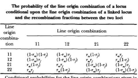
TABLE 2

The probability of the line origin combination of a locus conditional upon the line origin combination of a linked locus

and the recombination fractions between the two loci

Line -

origin Line origin combination

combina-

tion 11 12 21 22

(1-rmb/ ( 1 4 &/) rmr/

z-rf)

U-rm)(l-rf) (I-rJr rmr/ 8 1 -r,) (l-rm)rf ( 1 - 7 ~ h-7~

11 12

21 rm(l-r,) 22

(l-rm)(l-?)) (1-r ) r rm(l-?))

Conditional probabilities for the line origin combinations given in Table 1. The recombination frequencies between the pair of loci in the male and female parent are r,,, and rp respectively.

Once the possible line origin combinations of the markers have been derived, the probabilities of each of the four line origin combinations for a QTL at a given position in an F2 individual can be calculated condi- tional upon the possible line origin combinations of the markers, the previously estimated recombination frac- tions between the markers and the recombination frac- tion between the assumed position of the QTL and the markers. Table 2 gives the probability of the line origin combination of a locus conditional upon the line origin combination of a linked locus and the recombination fraction between the two loci. The probabilities in Table

2

have been written allowing for different recombina- tion rates in the two sexes; when these are the same Table 2 can be simplified. For each individual, each sec- tion of chromosome between pairs of markers which both have only a single possible line origin combination can be considered separately (as, in the absence of in- terference, markers outside this section provide no in- formation about the line origin of positions within the section). The probability of each of the four line origin combinations for any point between these markers (2. e.,

the position of a putative QTL) conditional upon the ob- served marker genotypes can be calculated as a product of the probabilities shown in Table 2 for any possible com- bination of line origins of the markers scaled so that the total over all possible combinations sums to one. The for- mal derivation of this method is shown in the APPENDIX.

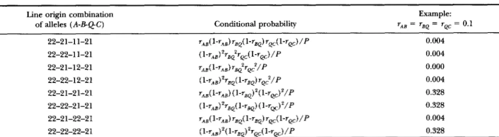
To clarify the calculation of these conditional prob- abilities, consider the example in Table 3. Marker loci

A, B and C are used (these correspond to markers A, B

and C for the pedigree of the F, individual shown in Table 1). Note that as markers A and C are fully infor- mative, with only a single line origin combination each, markers outside this region add no further information for positions within the region for this individual. Con- sider there to be a QTL ( @ at the midpoint between markers B and C. The first possible combination of line origins shown in Table 3 for the three markers and the QTL is 22,21,11 and 21 for A, B, Qand C, respectively.

As shown in Table 2, the conditional probability of a 21 line origin combination at marker B given a 22 line ori-

gin combination at marker A is (1 - rABm) rABr where r,,,

and rABf are the recombination fractions between loci A

and B in males and females, respectively. (This combi- nation of line origins at markers A and B requires there to have been no recombination between markers A and B in the first (male) F, parent and a single recombina- tion between the markers in the second (female) F, par- ent). Similarly, the conditional probability of a 11 line origin combination at the QTL given a 21 line origin combination at marker B is rBQm(l

-

rBw) and the con- ditional probability of a 21 line origin combination at marker C given a 11 line origin combination at the QTL is rQcT"( 1 - rQcr). The probability of the line origin com- binaoons 2 1 , l l and 21 at B, Q and C conditional on a 22 line origin combination at A is thus the product of these probabilities:

(1

-

rAB&AB/ra,(l - rBcu)rQcm(l

-

rQc/)

or:

(1 - rdrAB rBQ(1 - r,Q)rQc(l

-

rQJ

on the assumption of equal recombination frequencies in males and females. Division by the sum of these prob- abilities for the possible line origin combinations (eight are possible in the example in Table 3) gives the prob- ability conditional on the possible line origin combina- tions (and thus on the observed marker genotypes).

Once the conditional probabilities for the line origin combinations have been calculated the coeffkients for

a and d for a putative QTL in this position can be de- termined as:

a : probability of line origin 11 conditional on the marker genotypes minus probability of line origin 22 conditional on the marker genotypes

d : probability of line origin 12 conditional on the marker genotypes plus probability of line origin 21 conditional on the marker genotypes

or in the notation used in the APPENDIX:

a : prob(o,, I

P)

-

prob(o,, I

P)

and

d : prob(o,, I

P)

+

prob(w,, I

P)

where prob(w, I

P)

is the probability of line origin com- bination i for a QTL at a given position conditional on the observed marker genotypes in the individual and its parents and grandparents.

After calculation of the predicted coefficients for a putative QTL in a given position for all individuals, a and d can be estimated for that position by ordinary least squares, regressing the phenotypic values on to these coefficients. Several (or many) putative QTLs in a number of positions (linked or unlinked) can be fit- ted simultaneously and covariates or fixed effects can also be included in the model. For a fixed position of

QTL Mapping in Outbred Line Crosses

TABLE 3

1199

Example calculation of the probabilities of line origin combinations of a putative QTL conditional upon the possible line origin

combinations of flanking markers

Line origin combination Example:

of alleles ( A - B Q C ) Conditional probability rAB = rBQ = rQc = 0.1

22-21-11-21 ~ A B ( 1 - ~ A B ) ~ B ~ ( 1 ~ ~ B ~ ) ~ ~ c ( l - r ~ c ) / P 0.004

22-21-12-21 rBQ2rQc2/P rAB(1-rAB) 0.000

22-22-12-21 ( 1 - ~ A B ) 2 ~ B ~ ( 1 - ~ g ~ ) ~ ~ c 2 / P 0.004

22-21-21-21 ‘AB(l%B) (l-rBQ)z(l-rQC)z/P 0.328

22-22-21-21 (l-rAB)zrBQ(l-rBQ) (1-rQc)2/P 0.328

22-21-22-21 rAB(l-rAB)~BQ(l-rBq)rQc(l-rQc)/P 0.004

22-22-22-21 (1-rAB)2(1-rB,)2rQc(l~rQc)/P 0.328

22-22-11-21 0.004

For this individual the line origin combination (as defined in Table 1) of the first marker ( A ) is 22, that of the second marker ( B ) may be either 21 or 22 and that of the third marker ( C) is 21. The putative QTL (4) is placed between B and C. The recombination frequencies are assumed to be the same in both sexes and that between A and B is rAB, that between B and the putative position of the QTL is rBe and that between the QTL and C is rQc. Pis the sum of the numerators of the conditional probabilities. An example is given for rAB = rBQ = rQC = 0.1, For this individual the predicted coefficient for a would be -0.324 ( = 0.004

+

0.004 - 0.004 - 0.328) and for d would be 0.660 (= 0.000

+

0.004

+

0.328

+

0.328).

residual mean square provides the usual variance ( F )

ratio test statistic.

An alternative approximate log-likelihood ratio test statistic is provided by:

residual sum of squares reduced model

n log.( residual sum of squares full model

)

where n is the number of observations. This test statistic is distributed approximately as a chi-square with degrees of freedom equal to the number of parameters included in the full model (2. e . , estimating the QTL effects) but omitted from the reduced model ( i . e . , omitting QTL) (AITKEN et al. 1989). Dividing this test statistic by (210gJO) would approximately give the LOD score. The use of LOD is of little relevance, however, for tests such as this which have more than a single degree of freedom. When fitting a single QTL any of these test statistics can be plotted against position to give a curve or when fitting two QTLs this can be visualized as a surface (HALEY and KNOTT 1992). The maximum point of the curve or surface indicates the most likely position of the QTL and this point will be at the same position for any of the test statistics. We use the approximate log- likelihood ratio test statistic throughout this paper for consistency and to facilitate comparison with our pre- vious work ( e . g . , HALEY and KNOTT 1992; KNOTT and

HALEY 1992a, b)

.

SIMULATIONS

General: The analysis of simulated data was used to explore the characteristics of the method. Each set of data included 500 F2 individuals in 50 full-sib families of size 10 with their parents and grandparents. The geno- type of each individual comprised a pair of chromo- somes 100 cM in length. Depending upon the simula- tion there were either three markers at 50 cM spacing,

six markers at 20 cM spacing or eleven markers at 10 cM spacing. Markers of three types were generated, either fixed for alternative alleles in the two grandparental lines ( i . e., as in a cross between inbred lines), or seg- regating with the same two alleles at equal frequency in both grandparental lines or segregating with the same four alleles at equal frequency in both grandparental lines. QTLs ofvarious effect and position were simulated

(see below). In the analyses the additive and dominance effects ( a and d, respectively) of a single QTL were es- timated sequentially at each 1 c M point along the chro- mosome, with the distance between the markers set at that used to generate the data. The point along the chro- mosome at which the test statistic was highest was used to provide the estimates of the QTL position and effect for that analysis. Unless otherwise stated, 100 replicates were simulated and analyzed for each combination of parameters. The data were generated and analyzed us- ing programs written in FORTRAN 77, supplemented with routines from the NAG library (Numerical Algo- rithms Group 1990) for random number generation and for ordinary least squares analysis (routine G02DAF).

AU

markers us. flanking markers and size of QTL: To explore the general properties of the method and the advantage of using all markers on a chromosome, its behavior was compared to ordinary least squares in which only the pair of markers flanking an interval was used to predict the probabilities of each QTL genotype at a given point within the interval. For each replicate in these analyses a single set of phenotypic data (including effect of QTL and residual variance) was generated with a QTL of additive effect ( i e . , half the difference be- tween the homozygotes) of either 0.25, 0.5 or 1.0 re- sidual ( L e . , within QTL genotype) standard deviations

1200 C. S. Haley, S. A. Knott and J.-M. Elsen

-

0

m - Fixed for different alleles

r . . . 2 alleles segregating

-

all markers

-.-. 4 alleles segregating

-

all markers

" 2 alleles segregating

-

flanking markers

-...-

4 alleles segregating -flanking markers

0

z -

0 ln

ln 0

ln

.-

c c

c

.-

c

F

s -

"""_

I I I I I I

0 20 40 60 80 100

Position on chromosome (cM)

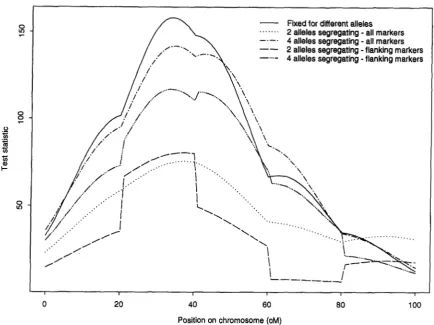
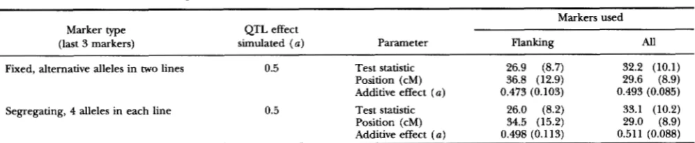
FIGURE 1.-Examples of test statistic curves using either only flanking markers or all markers. For each analysis markers were all of one of three levels of information content (fixed for alternative alleles in the two lines, or segregating with either two or four alleles at equal frequency in both lines) and were spaced at 2 k M intervals starting at 0 cM. The simulated QTL was additive in effect with two residual standard deviations between homozygotes and was located at the 3 k M position on the chromosome. The phenotypic data were the same for all analyses.

sizes would account for 3.396, 11.1% or 33.3%, respec- tively, of the variance in the F, population. Each set of phenotypic data was analyzed with markers at 20cM spacing which were all of one of the three levels of in- formation content (i.e., k e d for alternative alleles in the two grandparental lines or segregating with either the same two alleles at equal frequency or with the same four alleles at equal frequency in the two grandparental lines).

Marker density: Data were generated with a

QTL

with an additive effect of 0.5 residual standard deviation at 25 cM from one end of the chromosome. Each set of data had markers of the three levels of information content at either

l k M spacing or at 5 k M spacing and were analyzed using information from all markers simultaneously.

Position of QTL: Data generated with a

QTL

with an additive effect of 0.5 residual standard deviations at ei- ther 10 or 50 cM from one end of the chromosome. Each set of data had markers of the three levels of information content at 20cM spacing and were analyzed using in- formation from all markers simultaneously.

Markers of varying information content: In these analyses markers varied in their information content along the chromosome. Data were generated with a

QTL

with an additive effect of 0.5 residual standard de-

viations at 30 cM from one end of the chromosome and markers at 2 k M spacing. For each set of data the first three markers (at positions 0,20 and 40 cM) were of low information content ( i. e., the same two alleles at equal frequency segregating in each grandparental line) and the last three markers (at 60, 80 and 100 cM) were of higher information content (all three either having four alleles at equal frequency segregating in the grandpa- rental lines or being fixed for alternative alleles in the grandparental lines). The data were analysed using ei- ther information only from flanking markers or using information from all markers simultaneously.

Null hypothesis: Data were generated with no

QTL

but with markers at either

lo-,

20- or 50cM spacing. For each marker density, markers of the three levels of in- formation content were used to analyze the data. The data were analyzed using information from all markers simultaneously. For each combination of parameters 1000 replicates were generated and analyzed.

RESULTS

QTL Mapping in Outbred Line Crosses 1201

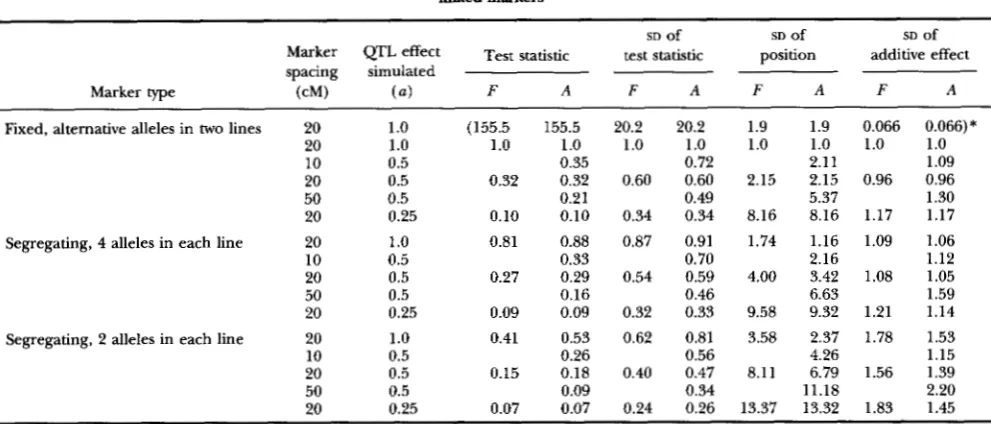
TABLE 4

Relative mean test statistics and empirical standard deviations of parameter estimates using either only flanking markers or all

linked markers

SD Of

Marker QTL effect T~~~ statistic test statistic

spacing simulated

position additive effect

SD Of SD Of

Marker type (cM) (a) F A F A F A F A

Fixed, alternative alleles in two lines 20 1.0 (155.5 155.5 20.2 20.2 1.9 1.9 0.066 0.066)*

20 10

1.0 1

.o

1.0 1.0 1.0 1.0 1.0 1.0 1.0

0.5 0.35 0.72 2.11 1.09

20 50

0.5 0.32 0.32 0.60 0.60 2.15 2.15 0.96 0.96

0.5 0.21 0.49 5.37 1.30

20 0.25 0.10 0.10 0.34 0.34 8.16 8.16 1.17 1.17

Segregating, 4 alleles in each line 20 1

.o

0.81 0.88 0.87 0.91 1.74 1.16 1.09 1.06

10 0.5 0.33 0.70 2.16 1.12

20 0.5 0.27 0.29 0.54 0.59 4.00 3.42 1.08 1.05

50 0.5 0.16 0.46 6.63

20

1.59

0.25 0.09 0.09 0.32 0.33 9.58 9.32 1.21 1.14

Segregating, 2 alleles in each line 20 1

.o

0.41 0.53 0.62 0.81 3.58 2.37 1.78 1.53

10 0.5 0.26 0.56 4.26 1.15

20 50

0.5 0.15 0.18 0.40 0.47 8.11 6.79 1.56 1.39

0.5 0.09 0.34 11.18 2.20

20 0.25 0.07 0.07 0.24 0.26 13.37 13.32 1.83 1.45

~ ~ ~ _ _ _ _ _ _ _ _ _ _ _ _ _ _ _ _ _ _

F, A, analyses using flanking or all markers, respectively. Each value is based upon 100 replicate simulations. Simulated QTLs were located 30

cM from one end of the 100-cM chromosome with 20-cM spaced markers or 25 cM from one end of the 100-cM chromosome with 10- and 50-cM

spaced markers. Simulated QTLs were additive in effect. The sue of the additive effect ( a ) of the QTL is given as half the difference between the homozygotes in terms of the residual (ie., within QTL genotype) standard deviation.

*

Absolute values this line only, all other values are given relative to these.

against the chromosomal position are shown in Figure

1. These curves were produced from a single set of phe- notypic data analysed using markers of one of the three levels of information content at 20-cM spacing and ei- ther predicting the QTL genotype using just flanking markers or using all markers on the chromosome. The two curves (usingjust flanking markers or using all mark- ers) produced when the markers were fixed for alter- native alleles in the two lines are exactly the same, con- firming that the flanking markers contain all the information on the interval between them for this type of marker under the assumption of no interference. For the less informative markers the use of just flanking markers produces steps in the curve between intervals and the maximum value of the test statistic reduces with the information content of the markers. The steps result because the different markers, and hence intervals, vary by chance in the information they contain. The use of

multiple markers to predict the QTL genotype removes these steps and also increases the test statistic, although the maximum test statistic still increases with increasing marker information content.

For data in which the markers in a linkage group were all of the same type, estimates of position and effect of the QTL for the analyses using either all markers or just flanking markers were very close to those simulated and are not shown. The relative values of the mean (over replicate simulations) of the maximum test statistic on the chromosome and the empirical (over replicate simu- lations) standard deviations of estimates of position and additive effect for the analyses using either all markers or just flanking markers are shown in Table 4 for these

analyses. Trends for the dominance effect were similar to those for the additive effect and are not shown. When the markers were fixed for alternative alleles in the two grandparental breeds, the results from analyses using all or flanking markers were, as expected, identical. For the less informative markers using all markers in the analysis generally increased the maximum test statistic. The larg- est increase (approximately 30%) was found for the least informative markers and for the QTL of largest effect, whereas for the QTL of smallest effect, no increase in the maximum test statistic was observed when using all markers rather than just flanking markers. The empiri- cal standard deviation of the estimates of position and effect was decreased for markers which were not com- pletely informative by using all markers in the analysis. For position, the magnitude of the decrease in the em- pirical standard deviation was greatest for the QTL of largest effect, but for the additive effect the magnitude of the decrease in the empirical standard deviation was greatest for the QTL of smallest effect.

1202

0 m

0

"

m

m

e o " N

.-

.- c _c

c

I-"

z

C. S. Haley, S. A. Knott and J.-M. Elsen

Markers at positions 60,80 and 100 cM

-

Fixed for alternative alleles

-

all markers

4 alleles segregating

-

all markers

4 alleles segregating

-

flanking markers

. . . Fixed for alternative alleles -flanking markers

"I-"

0 20 40 60

1

80 100

Position on chromosome (cM)

FIGURE 2.-Examples of test statistic curves using either flanking markers only or all markers and markers which vary in infor-

mation content along the chromosome. In both cases markers at positions 0,20 and 40 cM were of relatively low information content (two alleles at equal frequency in the two lines) and those at positions 60,80 and 100 cM were of relatively high information content (case 1: with four alleles at equal frequency segregating in the two lines or case 2: fixed for alternative alleles in the two lines). The simulated QTL was additive in effect with one residual standard deviation between homozygotes and was located at the 30 cM position on the chromosome. The phenotypic data were the same for all analyses.

two lines). This difference can be explained by the fact that an increase in marker density when markers are not com- pletely informative increases the probability that a QTL is flanked by informative markers, whereas this is not the case if the markers are already completely informative.

Position of Qm The mean of the maximum test sta- tistic on a chromosome and estimates of position and effect for the analyses using all markers at 20cM spacing were little affected by the position of the QTL no matter what the information content of the markers. For a QTL at 10 and 50 cM, respectively, the mean maximum test statistics over 100 replicates were 50.3 and 48.2 for mark- ers fixed for alternative alleles in the two lines, 27.9 and

29.2 for markers with the same two alleles at equal fre-

quency in the two lines and 44.2 and 43.4 for markers with the same four alleles at equal frequency in the

two lines. Thus for this marker spacing, position of the QTL has little effect on the power of its detection, despite a QTL at the centre of the chromosome hav- ing a greater chance of being flanked by two infor- mative markers.

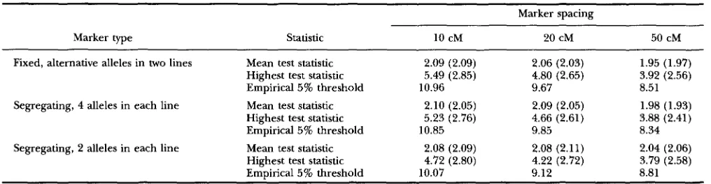
Markers of varying information content: Examples of the curves produced by plotting the values of the test

statistic against the chromosomal position when mark- ers vary in information content along the chromosome are shown in Figure 2. These curves were produced from the analysis of data in which there was a QTL at 30 cM and the first three markers had the same two alleles segregating at equal frequency in the two grandparental breeds and the last three markers were of higher information content (either four alleles segregating in both breeds or fixed for alternative alleles in the two breeds). In these analyses the use of just flanking markers results in the highest test sta- tistic being in the third interval, which is the first interval to be flanked by a marker of relatively high information content. Analyzing the same data using all markers results in the highest test statistic being in the second interval, which contained the simulated QTL.

The mean maximum test statistics and estimates of

QTL Mapping in Outbred Line Crosses 1203

TABLE 5

Mean test statistics and parameter estimates with markers varying in information content along the chromosome

Markers used Marker type QTL effect

(last 3 markers) simulated ( a ) Parameter Flanking All

Fixed, alternative alleles in two lines 0.5 Test statistic 26.9 (8.7) 32.2 (10.1)

Position (cM) 36.8 (12.9) 29.6 (8.9)

Additive effect ( a ) 0.473 (0.103) 0.493 (0.085)

Segregating, 4 alleles in each line 0.5 Test statistic 26.0 (8.2) 33.1 (10.2)

Position (cM) 34.5 (15.2) 29.0 (8.9)

Additive effect (a) 0.498 (0.113) 0.511 (0.088)

Each mean is based upon 100 replicate simulations and analyses and is shown with its empirical standard deviation over the replicates in

parentheses. All simulated QTLs were located 30 cM from one end of a 100-cM chromosome with 20-cM spaced markers and were additive in

effect. In each case the first three markers on the chromosome (at 0, 20 and 40 cM) were relatively low in information content, with the same

two alleles at equal frequency segregating in both grandparental lines, and the last three markers (at 60,80 and 100 cM) were more informative.

The size of the additive effect ( a ) of the QTL is given as half the difference between the homozygotes in t e r m s of the residual ( i . e . , within QTL genotype) standard deviation.

position of the QTL and increases the mean maximum test statistic.

Null hypothesis: Results of the analyses of data gen- erated with no QTL but with markers at either lo-, 20- or 50-cM spacing are shown in Table 6. For all marker densities and markers of different information content a test performed at a fixed position on the chromosome has a mean and a standard deviation of close to 2, as expected for a test statistic distributed as a chi-square with 2 d.f. (2 d.f. as both an additive and a dominance effect have been estimated). The mean over replicates of the highest test statistic on the chromosome increases both with increasing marker density and with marker information content. The approximate empirical 5% threshold calculated from these simulations as the mean of the 50th and 51st highest test statistics over replicates is also shown in Table 6; this value increases with marker density but shows no consistent trend with marker in- formation content.

DISCUSSION

The explosion in the availability of molecular genetic markers and the rapid development of linkage maps based on these markers is providing the geneticist with new tools to explore the genome (SOLLER and BECKMANN 1988; TANKSLEY et al. 1989). Interval mapping (LANDER and BOTSTEIN 1989) has proven to be a powerful tool for the dissection of some of the genetic factors underlying quantitative genetic variation in crosses between inbred lines ( e . g . , PATERSON et al. 1988,1991; JACOB et al. 1991; STUBER et al. 1992). As more species become amenable to this form of probing, however, statistical tools are needed to analyze a wider range of types of population. We have shown here that, as is the case for crosses be- tween inbred lines (HALEY and h o r n 1992), a simple ordinary least squares method can be applied to the analysis of populations resulting from crosses between outbred populations which are fixed for alternative QTL alleles.

The least squares method is relatively simple to apply and can extract most of the information contained in multiple linked markers. The use of all the markers in a linkage group simultaneously increases the test statis- tic, and thus the power for the detection of QTLs. It also removes bias in the estimated position and effect of a QTL which can result when markers vary in information content and are only considered a pair at a time [Table 5 and &om and H A L E Y (1992b)l.

The prediction of the QTL genotype using all markers in a linkage group is more diffkult than the use ofjust the flanking markers, which is all that is required for crosses between inbred lines. Thus programming the entire analysis in the language of a single statistical pack- age, as is possible for inbred lines (HALEY and horn

1992), becomes intractable. Once the predicted QTL genotypes have been calculated using a custom written computer program, however, these can be stored and the remainder of the analysis performed using a general statistical package.

The least squares analysis is very rapid and the time taken for computation does not increase greatlywith the number of parameters estimated, as it does in many maximum likelihood analyses. Thus the great advantage of least squares methods, other than their simplicity, is that many parameters can be fitted simultaneously. This first allows the inclusion of fixed effects such as treat- ment or sex in the model. Second, when exploring one chromosome, background genetic noise attributable to the other chromosomes can be reduced by the inclusion of QTLs at reasonable (say 30-50 cM) intervals down the remaining chromosomes in the model [e.g., JANSEN

1204 C. S. Haley, S. A. Knott and J.-M. Elsen

TABLE 6

Test statistic distribution under the null hypothesis

Marker spacing

Marker type statistic 10 cM 20 cM 50 cM

Fixed, alternative alleles in two lines Mean test statistic 2.09 (2.09) 2.06 (2.03) 1.95 (1.97) Highest test statistic 5.49 (2.85) 4.80 (2.65) 3.92 (2.56) Empirical 5% threshold 10.96 9.67 8.51

Segregating, 4 alleles in each line Mean test statistic 2.10 (2.05) 2.09 (2.05) 1.98 (1.93) Highest test statistic 5.23 (2.76) 4.66 (2.61) 3.88 (2.41) Empirical 5% threshold 10.85 9.85 8.34

Segregating, 2 alleles in each line Mean test statistic 2.08 (2.09) 2.08 (2.11) 2.04 (2.06) Highest test statistic 4.72 (2.80) 4.22 (2.72) 3.79 (2.58) Empirical 5 % threshold 10.07 9.12 8.81 The mean test statistic is based upon the mean of 101 positions (l-cM intervals on a 100-cM chromosome) over 1000 replicate simulations and analyses. The empirical standard deviation of the test statistic over the 1000 replicates averaged over the 101 positions is shown in parentheses. The highest test statistic represents the mean over 1000 replicates and its empirical standard deviation over the replicates is given in parentheses. The empirical 5% threshold is calculated as the mean of the 50th and 51st highest test statistics over the 1000 replicates.

or three linked QTLs.) This can remove bias introduced when linked QTLs are present but only a single QTL is fitted in the analysis (HALEY and KNOTT 1992; KNOTT and HALEY 1992a; MARTINEZ and CURNOW 1992). Fourth, more complex models of QTL gene action can be ex- plored relatively easily, for example two locus epistasis (HALEY and KNOTT 1992). Finally, using the same pre- dicted probabilities of QTL genotype the data could be analyzed using a generalized linear model, which is again possible in a number of statistical packages [e.g., AITKEN et al. (1989)l. This would allow QTLs underlying non-continuously distributed traits, such as binomial threshold traits, to be detected and mapped.

The need for the outbred populations to be fixed, or nearly so, for alternative QTL alleles may be considered restrictive, but in fact many populations may be of this type for some traits. Such populations would include divergently selected experimental lines and breeds with very different selection histories. When the populations crossed are not fixed for alternative QTL alleles, the power to detect a QTL will be increasingly reduced and its effect will be increasingly underestimated as the QTL allele frequencies in the two populations become more similar. The ability to detect only QTLs which differ in allele frequency between two populations may not be a great disadvantage in some circumstances, particularly when it is desired to detect favorable alleles found in one breed for introgression into a second. In fact the least squares method could be modified to detect QTLs which were segregating at intermediate frequencies in the populations which were crossed. Such QTLs would result in there being an interaction between the esti- mated effect of the QTL and F, family and such an in- teraction could be included in a least squares analysis. The detection of such an interaction, however, would require the use of F, families of reasonable size.

The simple method we have used here to predict prob- abilities of Q X genotypes does not extract all possible in- formation from the markers. There is a potential loss of information when both an F, parent and its parents are

heterozygous for the Same alleles and thus it is not possible to simply infer from which of these grandparents an F, individual inherits an allele. The proportion of these non- informative heterozygous parents is not expected to be greater than 0.125 (for markers at which the same two alleles are segregating at equal frequency in the grandpa- rental lines) and will often be much less than this. In a recent analysis of data from a cross between two outbred pig breeds (the European Wild Boar and the Large White), across 70 markers (approximately equal numbers of pro- tein polymorphisms, RFLps and mini or microsatellites) the average heterozygosity in the F, animals was 0.60 with less than 0.01 of these being non-informative heterozy- gotes (L. ANDERSON, personal communication).

Some of the information lost from non-informative heterozygotes by the simple method used here to infer genotype could be retrieved by the use of maximum likelihood methods to infer parental phase if there is data available on contemporary F, individuals (e.g., full or half-sibs). However, the extra information gained is likely to be slight, in part because non-informative het- erozygotes will often be relatively rare and also because the use of all markers means that some of the informa- tion lost is retrieved from informative flanking markers. LANDER and BOTSTEIN (1989) suggested an approxi- mation for the predicted size of the test statistic from interval mapping with a QTL responsible for a propor- tion

p

of the total variance, midway between two markers a recombination fraction of 8 apart in a sample of size

N . This approximation is equivalent to:

[(l - 28)/(1 - ~>lNlog,[l/(l -

$41

QTL Mapping in Outbred Line Crosses 1205

shows that this relationship appears to hold for markers which are less informative. The above formula predicts that reducing the distance between markers from 20 to 10 cM will increase the test statistic by around 12%, which is about the increase observed for the most in- formative markers. When the markers are less informa- tive, increasing their density has greater effect, the in- crease in the test statistic for the least informative markers being around 38% for the same change in marker spacing.

For the sake of consistency with previous work, we have chosen to use the approximate log-likelihood ratio test statistic rather than the F-ratio test statistic in this study. In practice familiarity might lead to the use of the F-ratio test statistic, but for neither of these test statistics is the distribution under the null hypothesis well un- derstood when multiple correlated tests are being per- formed. Thus which ever test statistic is chosen it will probably be necessary to probe the null hypothesis dis- tribution using simulation. The limited simulations of the null hypothesis situation which we have performed bear out the results of LANDER and BOTSTEIN (1989) in that the mean highest test statistic on achromosome and the 5% significance threshold increases with marker density. The mean highest test statistic on a chromo- some also increases with marker information content but the trend in the 5 % significance threshold value is not so clear cut. In practice both marker density and marker information content will vary from experiment to experiment and even between different regions of the genome. Thus it will probably be necessary to use Monte- Carlo methods to derive an approximate genome wide threshold for a chosen level of false-positives for each experiment. The least squares method lends itself to this approach because for a given set of marker data the probabilities of QTL genotypes at each position in each individual need only be derived once and stored. Then the phenotypic data can be simulated repeatedly and analysed by least squares. Nonetheless, even the modest number of 1000 replicate simulations and analyses for the 1500 1 c M spaced analyses in a 15-Morgan genome would be quite time consuming.

For slow breeding plant or animal species, especially those that suffer severely from inbreeding depression, the production of inbred lines prior to the establish- ment of a QTL mapping study is not an option. For other species, such as mice, it is an option, albeit a relatively slow and costly one. The advantage of inbreeding is that any markers that are useful in the cross between the inbred lines will be fixed for alternative alleles in the two lines and thus fully informative as will any segregating QTLs. However, some markers that would have been partially informative in the cross between outbred lines may be fixed for the same allele and thus become non- informative in the inbred line cross. To take an extreme example, consider markers at lOcM intervals with two alleles at equal frequencies in each of the two outbred

lines. Inbreeding these lines would result in one fully informative marker on average every 20 cM (as half of the markers are expected to be fixed for different alleles and half for the same allele). In this case our results (Table 4) suggest that producing inbred lines would re- sult in a more powerful test for the QTL. Most markers, however, are likely to be more informative in the cross between the outbred lines than in the example given above (as drift alone is likely to have made the allele frequencies differ between the lines), and so the choice based upon power alone is not likely to be clear-cut. Often other considerations, such as time and cost, will preclude the use of inbreeding making a cross between outbred lines the only viable solution.

C.S.H. and S.A.K acknowledge support under the Agncultural and Food Research Council (AFRC)-Institut National de la Recherche Agronomique (INRA) fellowship scheme for their stay in Toulouse.

This work was also supported by the AFRC and the Minisq of Agri-

culture, Fisheries and Food in the United Kingdom and is part of the Pig Gene Mapping Project which is supported by the BRIDGE pro-

gramme of the Commission of the European Communities.

LITERATURE CITED

AITKEN, M., D. ANDERSON, B. FRANCIS and J. HINDE, 1989 Statistical

Modelling in GLZM. Oxford University Press, Oxford. BECKMANN, J. S., and M. SOLLIX, 1988 Detection of linkage between

marker loci and loci affecting quantitative traits in crosses between segregating populations. Theor. Appl. Genet. 7 6 228-236.

HALEY, C. S., and A. L. ARCHIBALD, 1992 Porcine genome analysis, pp.

99-129 in Genome Analysis Vol. 4: Strategies for Physical Map- ping, edited by K. E. DAVIES and S. E. TILGHMAN. Cold Spring Har-

bor Laboratory, Cold Spring Harbor, N. Y.

H A L E Y , C. S., and S. A. KNOTT, 1992 A simple regression model for interval mapping in line crosses. Heredity 6 9 315-324.

JACOB, H. J., K L I N D P A I ~ R , S . E. LINCOLN, K KUSUMI, R. K. BUNKER et al.,

1991 Genetic mapping of a gene causing hypertension in the stroke-prone hypertensive rat. Cell 67: 213-224.

JANSEN, R. C., 1992 A general mixture model for mapping quanti-

tative trait loci by using molecular markers. Theor.-Appp'i. &net.

85: 252-260.

KNOIT, S. A, and C. S. m y , 1992a Aspects of maximum likelihood

interval mapping in an F, population. Genet. Res. 60: 139-151.

KNOTT, S. A., and C. S . HALEY, 199213 Maximum likelihood mapping

of quantitative trait loci using fullsib families. Genetics 130:

1211-1222.

LANDER, E. S., and D. BOTSTEIN, 1989 Mapping Mendelian factors

underlying quantitative traits using RFLP linkage maps. Genetics

121: 185-199.

MARTINEZ, O., and R. N. CURNOW, 1992 Estimating the locations and the sizes of the effects of quantitative trait loci using flanking

markers. Theor. Appl. Genet. 85: 480-488.

NUMERICAL ALGORITHMS GROUP, 1990 The NAG Fortran Library

Manual-Mark 14. NAG Ltd., Oxford.

PATERSON, A. H., E. S . LANDER, J. D. HEWITT, S . PETERSON, S . E. LINCOLN

et a l . , 1988 Resolution of quantitative traits into Mendelian fac- tors, using a complete linkage map of restriction fragment length

polymorphisms. Nature 335: 721-726.

PATERSON, A. H., S . DAMON, J. D. HEWITT, D. ~ A M I R , H. D. RUIINOWCH

et al., 1991 Mendelian factors underlying quantitative traits in

ments. Genetics 127: 181-197.

tomato: comparison across species, generations and environ-

SOLLER, M., 1990 Genetic mapping of the bovine genome using

deoxyribonucleic acid-level markers to identify loci affecting quantitative traits of economic importance. J. Dairy Sci. 73:

SOLLER, M., and J. BECKMANN, 1988 Genomic genetics and the utili- zation for breeding purposes of genetic variation between popu- lations, pp. 161-168 in Proceedings of the 2nd International Conference on Quantitative Genetics, edited by B. S . WEIR,

1206 C. S. Haley, S. A. Knott and J.-M. Elsen

M. M. GOODMAN, E. J. EISEN and G . NAMKOONG. Sinauer Assoc., Sunderland, Mass.

STUBER, C. W., S. E. LINCOLN, D. W. W o w , T. HELENTJARIS and E. S. LANDER, 1982 Identifkation of genetic factors contributing to heterosis in a hybrid from two elite maize inbred lines using mo- lecular markers. Genetics 132: 823-839.

TANKSLEY, S. D., N. D. YOUNG, A. H. PATERSON and M. W. BONIERBALE, 1989 RFLP mapping in plant breeding: new tools for an old science. Biotechnology 7: 257-264.

Communicating editor: B. S. WEIR

APPENDIX

We consider a three generation family (Table 1) with four grandparents from two outbred lines (sire of sire,

SS; dam of sire,

DS;

sire of dam, SD and dam of dam,

DD),

two F, parents (sire, S and dam,

D )

and one F,

offspring ( 0). The seven members of the family are all typed for codominant markers at Iloci which have been already mapped. Let P be the vector of marker pheno- types. P comprises

7

X I terms.

We require the posterior probability, given P, of the grandparental origin w of the two alleles at any position in the genome for the offspring, prob ( w I P)

.

Notation: The vector of marker phenotypes, P, is sub- divided into seven sub-vectors,

P = (Po Ps PD Pss Pm PsD PDD )

with P, = (Ps

P

,

)

and P, = (P,, P,, P,, PDD). At a particular locus, the genotype of an individual is defined by an ordered couplet of digits with, in the first position the allele received from the sire and in the second po- sition the allele received from the dam. Avector of geno- types G , with 7 X

I

couplets, underlies the vector P.

Hence for an observation P with a total (over all marker loci in all seven individuals in the pedigree) of H het- erozygous loci there are 2H corresponding different pos- sible vectors G .

Let be a vector of grandparental origins of the I marker loci in the offspring,

a

= (fl,

a,

. .

.

aI).

ai

( i = 1

. .

.

I) represents the line origin combina- tion of the marker alleles and takes the value 11 when the offspring received the SS and SD alleles, 12

when SS and

DD,

21 when DS and

SD

and 22 when

DS

and

DD.

Result: If the markers are codominant and without missing data, assuming linkage equilibrium in the grandparents between the loci and no interference in recombination, the probability of the grandparental ori- gin at any position in the offspring genome, given the phenotypes P is:

prob(wI P ) = prob(w I aj)prob(aj+, I w)

X

n{=,

prob(LR,I

ai-,)

nf=i+2

prob(QI flj-,)

2 A g p I I 5 = 2 prob(aiI Q i - 1 )

with

j

I1

prob(aiI

ai-,)

= 1 when j = 1

i=2

and

I

fl

prob(QIfl-,) = 1 when j = I - 1.

i = j + 2

rp

being the whole set of consistent vectors considering the observations P and markers j

(1 5 j 5

I

- 1) and j + 1 bound the interval containing the putative QTL.

This is equivalent to:

prob(w I P)

That is, the required probability can be written in terms requiring only the recombination rate be- tween adjacent markers (prob(Qilfl,,) as given in Table 2) and between the putative QTL and its flank- ing markers.

Proof:

prob(w I P) = prob(w I aP)prob(a I P).

n

We will now consider the two components separately. First,

prob(w I

aP)

= prob (w I 0).

In the absence of interference in recombination, we have

prob(wl

a)

= prob(wl s Z j ,

aj+,)

(1)

where j and j

+

1 are the markers flanking the consid- ered position. Second,

prob(fl I P)

Rewriting in terms that are conditional on only parental and grandparental phenotypes gives:

prob(fl I P,, Pp)prob(PoI

a,

PBp, Pp>

prob(f2 I

P)

=

prob(a1 P,, P,,)prob(P,I

a,

P,, PPI '

The two component probabilities will now be consid- ered separately. First,

prob(fl I p,, PP)

= prob(a)

= prob(a,)prob(fl, I Ol)prob(a, I

a,,

a,)

.

.

. .

QTL Mapping in Outbred Line Crosses 1207

R2

. . .

= prob(RiI

a,,).

Thus

prob(Rl P,,P,)=prob(Rl)n~=,prob(Ril

ai-,).

(2)

The first term, prob(R,), is simply

i.

Second,

prWP, I ~,P,,P,>

Rewriting this probability to be conditional on the pa- rental genotypes gives:

probP, I

a,

P,, PPI

=

E

prob(P,I

R,

P,, Pp, G,)prob(G,I

a,

P,, PPI.

Gp

Again, we will consider the two components separately. First,

prob(Po I

R,

P,, P,, G,) = prob(P, I

52,

G,)

I (3)

=

n

prob(P,I

ai,

G,,). i= 1

Due to the o n e t w n e correspondence between ( R , Gpi) and G,, we have prob(P,I

R,

GJ = prob(P,I G,) which is 1 if phenotype and genotype are consistent and 0 otherwise. Second,

prob(G,I 0, p,, PPI = prob(G, I P,, P,)

= prob(Gs I P, 9 PDs 9 Ps)prob(GD I PSD 9 P D D 3 PD

1.

Consider the sire probability. Assuming linkage equilibrium in the grandparents and with a single progeny ( S ) , the events at each locus are indepen- dent, hence

I

prob(GsIPss, PDs, =

II

prob(GSi1 Pssi, PDsi, Psi). i= 1

(4)

Considering the zth locus, three situations are pos- sible, viz:

( S l ) GSi and Psi are not consistent, giving

(S2) G,, and Psi are consistent; Pssi, PDsi, Psi are not all heterozygous for the same alleles. The proba- bility is 1.

(S3) GSi and Psi are consistent; Pssi = PDsi = Psi are all heterozygous (say A B ) .

prob( G, = A B 1 Psi = PDSi = Psi = AB) prob( GSi I ps,'ji, 'DSi? psi) = 0.

= prob( Gs = BA I Pssi = PDsi = Psi = AB) =

.

Hence, combining the results from (3) and (4), we have

prOb(P0 I P,, Pp)

=

2

n

(prob(P,I

ai,

G,,)prob(G,,I PWi, Ppi))

G, i

=

n

prob(P,I a i , G,,)prob(G,,I P,,, P,,)

.

For any consistent

R,

and Gpi, the product (prob(P,I

ai,

G@)prob(G,,I P,,, P,,)) is a constant with a value of

:,

$

or 1, depending on the number of grandparent and parent trios that are heterozygous for the same genotype (z.e., 2, 1 or 0).

Additionally, there is only one possible G,, in the summation. This is obvious in situations S1 and S2,

above. In the situation S3, two G,, are consistent with P,, P,, and P,, but one only belongs to

r,.

If, for ex- ample, Ri = 11 and GDi = XU, the genotype G, = AB

gives an offspring phenotype AXand the genotype Gsi = BA gives an offspring genotype BX. If the observed phenotype P, was A A , Gsi = BA cannot be consistent; if it is AB, allele Xmust be A or B and only one of the

G, (depending on the GDi) is possible.

Hence prob(P, I

R,

P,, P,) is constant over all line origin combinations (0) consistent with P and it is equal

to ($", h being the number of grandparental and pa-

rental trios that are heterozygous for the same genotype over all loci, and for all other combinations is 0.

Combining this result with (2) we have the following expression for any possible R,

i (

(

+

1

nb,

prob(R,I

Ri-l)$h

prob(R I P) =

EaErp

HLz

p r o b ( ~ i ~ ~ i - l ) ( $ ~

and, incorporating the result from ( l ) , the probability we require can be written as follows:

prob(o I P)