ABSTRACT
RUTKOWSKI, DAVID MATTHEW. Simulations to Predict the Phase Behavior and Structure of Multipolar Colloidal Particles. (Under the direction of Dr. Carol K. Hall).
Colloidal particles with anisotropic charge distributions can assemble into a number of interesting structures including chains, lattices and micelles that could be useful in biotechnology, optics and electronics. The goal of this work is to understand how the properties of the colloidal particles, such as their charge distribution or shape, affect the self-assembly and phase behavior of collections of such particles. The specific aim of this work is to understand how the separation between a pair of oppositely signed charges affects the phase behavior and structure of assemblies of colloidal particles. To examine these particles, we have used both discontinuous molecular dynamics (DMD) and Monte Carlo (MC) simulation techniques.
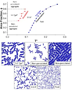
In our first study of colloidal particles with finite charge separation, we simulate systems of 2-D colloidal rods with four possible charge separations. Our simulations show that the charge separation does indeed have a large effect on the phase behavior as can be seen in the phase diagrams we construct for these four systems in the area fraction-reduced temperature plane. The phase diagrams delineate the boundaries between isotropic fluid, string-fluid and percolated fluid for all systems considered. In particular, we find that coarse gel-like structures tend to form at large charge separations while denser aggregates form at small charge separations, suggesting a route to forming low volume gels by focusing on systems with large charge separations.
structure, a theoretical structure with an infinite number of phase transitions, under specific conditions. The limit-periodic structure only forms when the rotation of the particles in the system is restricted to increments of π/3. When the rotation is restricted to increments of π/6 or the rotation is continuous, related structures form including a striped phase and a phase with nematic order. Neither the distance from the point charges to the center of the particle nor the angle between the charges influences whether the system forms a limit-periodic structure, suggesting that point quadrupoles may also be able to form limit-periodic structures. Results from these simulations will likely aid in the quest to find an experimental realization of a limit-periodic structure.
Next we examine the effect of charge separation on the self-assembly of systems of 2-D colloidal particles with off-center extended dipoles. We simulate systems with both small and large charge separations for a set of displacements of the dipole from the particle center. Upon cooling, these particles self-assemble into closed, cyclic structures at large displacements including dimers, triangular shapes and square shapes, and chain-like structures at small displacements. At extremely low temperatures, the cyclic structures form interesting lattices with particles of similar chirality grouped together. Results from this work could aid in the experimental construction of open lattice-like structures that could find use in photonic applications.
Simulations to Predict the Phase Behavior and Structure of Multipolar Colloidal Particles
by
David Matthew Rutkowski
A dissertation submitted to the Graduate Faculty of North Carolina State University
in partial fulfillment of the requirements for the degree of
Doctor of Philosophy
Chemical Engineering
Raleigh, North Carolina 2016
APPROVED BY:
______________________________ ______________________________
Dr. Carol K. Hall Dr. Keith E. Gubbins
Committee Chair
______________________________ ______________________________ Dr. Orlin D. Velev Dr. Erik E. Santiso
DEDICATION
BIOGRAPHY
ACKNOWLEDGMENTS
I would like to acknowledge and thank my PhD advisor, Dr. Carol Hall for guiding me throughout my graduate studies. I am particularly grateful to her for encouraging me to become more adept at public speaking and to focus my ideas as a writer. I would also like to thank Prof. Sabine Klapp, who advised me while I worked in Germany. Her insights and feedback will be missed. I am grateful to Dr. Josh Socolar for pointing out the importance of the structures I had found through earlier simulations and then giving me the benefit of his expertise on the double-dipole project. I wish to acknowledge the other members of my committee: Dr. Orlin Velev, Dr. Erik Santiso and Dr. Keith Gubbins for their helpful suggestions over the years. Specifically, I would like to thank Dr. Velev for the very useful discussions on experimental work and Dr. Santiso for several discussions on simulation. Finally, I am grateful to my collaborators, Dr. Bhuvnesh Bharti and Dr. Catherine Marcoux, for working with me on several interesting projects.
TABLE OF CONTENTS
LIST OF FIGURES ... ix
CHAPTER 1 ...1
Motivation and Overview ...1
1.1 Motivation ... 2
1.2 Overview ... 3
1.2.1 The Effect of Charge Separation on the Phase Behavior of Dipolar Colloidal Rods ...4
1.2.2 Formation of Limit-periodic Structures by Double-dipole Particles Confined to a Triangular Lattice ...4
1.2.3 Simulation Study on the Structural Properties of Colloidal Particles with Offset Dipoles ...5
1.2.4 Capillary Bridging as a Tool for Assembling Discrete Clusters of Patchy Particles ...5
1.2.5 Future Work...6
1.3 Publications ... 6
1.4 References ... 7
CHAPTER 2 ...9
The Effect of Charge Separation on the Phase Behavior of Dipolar Colloidal Rods ...9
2.1 Introduction ... 12
2.2 Methods... 19
2.3 Results ... 27
2.4 Discussion and Conclusions ... 31
2.5 Acknowledgements ... 36
2.6 References ... 37
Appendix 2-1 Discontinuous Potential Development... 53
CHAPTER 3 ...55
3.1 Introduction ... 57
3.2 Methods... 61
3.3 Results and Discussion ... 67
3.4 Discussion and Conclusions ... 75
3.5 Acknowledgements ... 78
3.6 References ... 79
CHAPTER 4 ...95
Simulation Study on the Structural Properties of Colloidal Particles with Offset Dipoles ...95
4.1 Introduction ... 98
4.2 Model and Methods ... 101
4.3 Results and Discussion ... 107
4.4 Conclusions ... 117
4.5 Acknowledgements ... 119
4.6 References ... 120
CHAPTER 5 ...134
Capillary Bridging as a Tool for Assembling Discrete Clusters of Patchy Particles ...134
5.1 Introduction ... 137
5.2 MC Simulation Details ... 139
5.2.1 Monodisperse interaction potential ...140
5.2.2 Interaction potentials for a mixture of 4μm and 2μm spheres ...141
5.3 Results and Discussion ... 141
5.3.1 Liquid-lipid driven particle clustering ...142
5.3.2 Thermal switching of clusters ...144
5.3.3 Monte Carlo simulations of patch particle clustering...145
5.3.4 Capillary bridging of complex particles and their mixtures ...148
5.4 Conclusions ... 149
5.5 Acknowledgments... 150
CHAPTER 6 ...166
Conclusions and Future Work ...166
6.1 Conclusions ... 167
6.2 Future Recommendations ... 169
6.2.1 Simulations in External Fields...170
6.2.2 3d Offset Dipolar Spheres ...171
6.2.3 Spheres with Four Embedded Point Dipoles ...172
LIST OF FIGURES
Figure 2.1. Model of 4:1 dipolar rod used in our DMD simulations incorporating seven spheres bonded together to represent the excluded volume of the rod and two smaller spheres shown in red and blue at the ends to represent the charges of the extended dipole. The outermost square wells for the
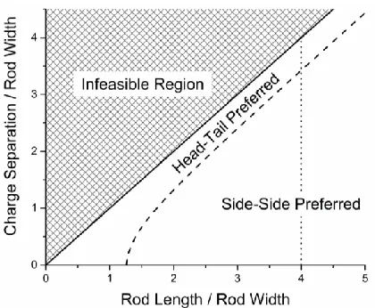
charged spheres are shown as dashed circles. ...43 Figure 2.2. Plot of charge separation versus rod length both reduced by the rod width,
which shows the regions where a head-tail pair of dipolar rods is preferred and where a side-side pair of dipolar rods is preferred. The dashed
conformation delineation line shifts slightly depending on the potential used to model the interactions between the charged groups in the dipolar rod. The hashed region is infeasible because it has charge separations that are longer than the rod itself. The dotted line indicates the aspect ratio at
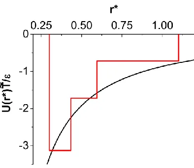
which the simulations in this paper were performed. ...44 Figure 2.3. Plot comparing the continuous Yukawa potential energy and our
discontinuous potential energy between charges of opposite sign versus the distance between the centers of the two charges. Charges with the same sign interact through a square shoulder that has the same energy boundaries and magnitudes, but has positive values of energy instead of
negative. ...45 Figure 2.4. Order parameters calculated in our simulations along with sample data
(blue points) and curves fit to the data (red lines). (a) The definition of percolation probability and an example of a percolated system. (b) The
definition of the extent of polymerization and an example of a string-fluid. ...46 Figure 2.5. (a) The definition of the head-tail order parameter and an image of a pair of
rods that are head-tail ordered. (b) The definition of the side-side order
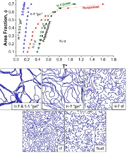
Figure 2.6. Phase diagram for 4:1 dipolar rods with charge separation of 3.7 plotted in the area fraction vs temperature plane. Fluid, string-fluid, H-T string-fluid, H-T “gel” and H-T & S-S ordered “gel” phases are present in this
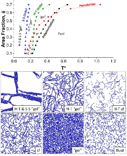
diagram. ...48 Figure 2.7. Phase diagram for dipolar rods with charge separation 3.5 plotted in the
area fraction vs temperature plane. Fluid, string-fluid, T string-fluid, H-T “gel”, “gel”, and H-H-T and S-S “gel” are present. ...49 Figure 2.8. Phase diagram of dipolar rods with 3.0 charge separation plotted in the area
fraction vs temperature plane. Fluid, string-fluid, S-S “gel” and H-T and
S-S “gel” are present. ...50 Figure 2.9. Phase diagram of dipolar rods with charge separation 2.5 plotted in the area
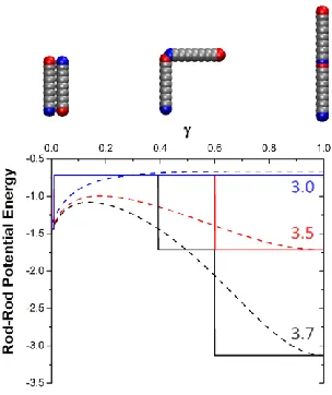
fraction vs temperature plane. Fluid, S-S string-fluid, and S-S “gel” are present. There is no H-T transition for this system; the rods always line up in S-S fashion. ...51 Figure 2.10. The rod-rod potential energy vs. “joint” angle curves for the Yukawa
potential (dashed lines) and our discontinuous potential (solid lines). The three-step discontinuous potential used in our simulations was derived by matching the rod-rod potential energy calculated for the continuous Yukawa potential with that for the discontinuous potential. Black, red and blue lines are for charge separation 3.7, 3.5 and 3.0, respectively. ...52 Figure 3.1. (a) Black-stripe model in which the specific pattern of lines induces the
formation of a limit-periodic structure upon slow temperature quench 11.
(b) Double-dipole disk model with four charges of alternating sign. The charges in play a similar role to the top and bottom lines in (a); the
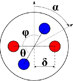
horizontal bar in (a) is however absent in (b). ...82 Figure 3.2. Double dipole disk model used in simulations where blue circles represent
by the angle α, which for the orientation shown is equal to π/3. The orientation is therefore positive for clockwise rotations and negative for
counterclockwise rotations. ...83 Figure 3.3. (a) Sublattice labeling with level-1 ordering shown in which sublattice A
contains rattlers whose orientations are not shown. (b) Mapping used to define the value of eX for an individual disk based on its orientation (up,
left or right) and sublattice (A, B, C or D) (Figure adapted from Ref 11).
The 3D arrows shown inside the tetrahedrons are the four possibilities for the unit vector eX. ...84
Figure 3.4. (a) Sublattice labeling with striped phase shown. (b) Mapping used to define the value of eK for an individual disk based on its orientation and sublattice (A, B, C or D). The 3D arrows shown inside the octahedrons are the six possibilities for the unit vector eK. ...85 Figure 3.5. Images of some of the non-limit-periodic-structures found in our
simulations. The gray spheres represent the excluded area of the disk but are shown at reduced size to better visualize the orientation of the disks. Striped phases have alternating bands of disks whose order is determined by the striped order parameter. These stripes can also occur for just the rattlers as shown in the second image. The unidirectional rattler phase is investigated by first measuring 1 on the entire system and then
calculating the nematic order parameter on the rattlers. ...86 Figure 3.6. Left: Image of a rattler (disk 6) and its surrounding six disks (disks 0-5)
refer to the two sublattices which contain disks which are rotated off of
their level-1 structure while D3 is the non-distorted sublattice. ...87
Figure 3.7. (a) Striped order parameter, 1, versus reduced temperature T* for
continuous rotation simulations. Values of δ are shown in the legend. (b)
1
(filled symbols and solid lines) and nematic order parameter (open symbols and dashed lines) for continuous rotation simulations. Values of δ are shown in the legend. ...88 Figure 3.8. 1 for 0.25 using the R6 moveset. Values in the legend indicate the
value of δ...89 Figure 3.9. 1 (a) and 2 (b) vs. T
* for 0.30 using the R6 moveset. Note the
difference in the horizontal scales on the two plots. Values in the legend
indicate the value of δ. ...90 Figure 3.10. Subset of the system (22x24 of a 64x64 system) at δ = 0.35 using the R3
moveset color coded according to the level the disks are in. Gray
corresponds to level-1, green to level-2, red to level-3, blue to level-4 and black is not ordered. The figure on the right plots n for these four levels
versus log(T*). ...91
Figure 3.11. Order parameters for four levels of order plotted versus T where gray
circles are for level-1, green crosses for level-2, red triangles for level-3
and blue x’s for level-4. ...92 Figure 3.12. State diagram showing the different phases found for a given moveset as a
function of δ. Red squares stand for striped phase, blue triangles for α-rattler phase, pink upside-down triangles for β-α-rattler phase, green diamonds for striped rattler phase and black circles for limit-periodic
phase. ...93 Figure 4.1. Model of the offset-dipole sphere used in this work. The large sphere
negative (blue) charges on the extended dipole. The charges do not, in
actuality, have a physical size and are pictured here as spheres for clarity. ...123 Figure 4.2. Cosine of the angle between two extended dipoles for two offset dipoles
confined to the x-y plane at their minimum potential energy (ground state) configuration as a function of the displacement, δ*. Lines represent
minimization of the pair potential energy as a function of δ* for either a point dipole (black) 23, Case 1 (red) and Case 2 (blue). Dashed lines are results for k=0 (Coulomb potential). Points are results from simulated
annealing MC simulations. ...124 Figure 4.3. Ground state structures for systems of three particles for both Case 1 and
Case 2. Images on the left show representative structures where the value below the image is δ* for the particle and the numbers in parenthesis for Case 2 are the angle θ. The plots on the right display the ∆ij for the three pairs of dipoles (∆12, ∆13, ∆23) as a function of δ*. Colors on the right plots highlight regions where the corresponding structures on the left are
the minimum energy structure. ...125 Figure 4.4 Ground state structures for systems of four particles for both Case 1 and
Case 2. Images on the left show representative structures where the number below the image is the value of δ* for the particle and the number in parenthesis for Case 2 is equal to θ. The plots on the right display the values of ∆ij as a function of δ*. Colors on the right plots highlight regions where the corresponding structures on the left are the minimum
energy structure...126 Figure 4.5. Plot showing the most stable cyclic structure as a function of the shift of the
dipole, δ* from the particle center, δ, for Case 1 and 2. ...127 Figure 4.6. Snapshots of low temperature systems at φ = 0.1 for d* = 0.01 systems.
above the percolation transition and T2 is a temperature below the
percolation transition for each system. ...128 Figure 4.7. a) Percolation and b) polymerization transition lines as functions of T for
Case 1. Numbers in the legends indicate the value of δ*. ...129 Figure 4.8. Snapshots of structures formed in finite temperature simulations using Case
2. T1 is a temperature below the polymerization transition but above the percolation transition and T2 is a temperature below percolation transition for each system. ...130 Figure 4.9. a) Percolation and b) polymerization transition lines as functions of T for
Case 2. Numbers in the legends indicate the value of δ* while those in the parenthesis indicate the value of θ. The open circles are the percolation transitions for the fused cyclic cluster simulations which are described
later. ...131 Figure 4.10. Fraction of particles that are in polygons, fc, as a function of δ* for a)
Case 1 and b) Case 2. Numbers in the legends indicate the area fraction
for each curve. These values were calculated for configurations at T2...132 Figure 4.11. Structures formed from fused cyclic cluster simulations for particles with
d* = 0.40 at an area fraction of 0.1. Values below the images indicate the
angle, θ, used in our model as shown in Figure 4.1. ...133 Figure 5.1. (a) A schematic summarizing the general methodology for fabricating lipid
patched polystyrene (PS) microspheres. (b) Interactions between all three surface-pairs of the patchy microparticle. Here the thickness of the liquid
fatty acid layer and particle size are not to scale. ...154 Figure 5.2. (a) Optical micrographs illustrating the self-assembly of lipid-wetted Janus
particles into ordered colloidal clusters in aqueous dispersion. The inset shows an SEM image of the Janus particles before assembly in the dried state. (b-e) Examples of 2D and 3D clusters formed by capillary binding
Figure 5.3. (a) The fraction of Janus particles self-assembled into clusters at different temperatures for ethanolamine salts of dodecanoic acid (squares) and n-hexadecanoic acid (circles). The vertical lines indicate the fluid-to-gel phase transition temperature (Tp) of the fatty acids on iron oxide surfaces.
(b) and (c) The clusters disassembled upon decreasing the temperature below the fluid-to-gel phase transition of the fatty acid, i.e. when the liquid in the capillary bridge freezes. At temperature T < Tp, the fraction of assembled particles remains negligibly small. The corresponding schematics illustrate thermally reversible capillary bridge formation and
rupturing. Scale bar in (b) 10 μm. ...156 Figure 5.4. (a) Self-assemblies formed by the patchy particles (f = 0.15) in Monte
Carlo simulations of the capillary assembly process. The inset shows an individual particle unit formed by distributing 252 domains on a central core. (b) Micrograph of patchy microspheres with fractional patch area of 0.15 assembled into low aggregation number clusters. (c-e) Surface interaction energy map for different patch sized particles (f = 0.50, 0.20, and 0.15). The attractive interaction between the lipid coated patches was modeled on the basis of a square-well attractive potential. (f) The increase in the fraction of assembled particles upon increasing the relative patch area (f) in simulations (filled circles) and experiments (open squares).
Scale bar in (b) 50 μm. ...157 Figure 5.5. (a-c) Micrographs of the assemblies formed by a mixture of 4 μm and 2 μm
Janus particles. (d-f) Capillary bridged self-assemblies formed by double-patched microspheres. The insets in the frames are the clusters observed in corresponding Monte Carlo simulations. Scale bar in each image is 2 μm. ...158 Figure 5.6. SEM image of the single patched particles with relative surface patch area
particles where two distinct triangular patches were introduced onto the particles surface by metal vapor deposition from diagonally opposite
sides. Scale bar = 4 μm. ...159 Figure 5.7. Determination of the zeta potential of iron oxide coated flat surface at pH
9.5. Here the zeta potential was determined by measuring the apparent zeta potential (or electrophoretic mobility) of tracer particles (-37 mV) away from the flat surface. The scattered points are experimentally
measured data points and the red linear fit to the points. ...160 Figure 5.8. Zeta potential of all surfaces present in the assembly dispersion. All the
surfaces were negatively charged at pH 9.5 and hence electrostatically
repulsive. ...161 Figure 5.9. Microscope images showing the dynamics of the self-assembly of Janus
particles driven by lipid mediated capillary bridging. Mean cluster
aggregation number increases as the assembly progresses. The kinetics of assembly is quantified in Figure 5.10. Scale in (c) = 50 μm. ...162 Figure 5.10. Monte Carlo simulation snapshots showing the near-equilibrium clusters
formed by patchy particles with surface patch fraction (a) f = 0.2, and (b) f = 0.5. The red-red patches were attractive, and red-blue and blue-blue
patches were repulsive. ...163 Figure 5.11. Kinetics of particle clustering for different patch sized particles (a-b) f =
0.15, (c-d) f = 0.20, (e-f) f = 0.50. Both MC simulations (b, d, f) and experiments (a, c, f) show similar qualitative behavior where particles assemble (or reassemble) into higher aggregation number clusters with
increasing assembly duration (or move number for simulations). ...164 Figure 5.12. Monte Carlo simulations snapshots for the equilibrium clusters formed by
(a) Mixture of dissimilar sized particles Janus particles (f = 0.5), and (b)
1.1 Motivation
Colloidal systems consist of particles on the order of nanometers to micrometers suspended in a carrier fluid. Due to their size, these particles are assumed to behave classically, yet they are small enough to be affected by Brownian motion. These particles can self-assemble into complex structures under the effects of Brownian motion and are therefore attractive candidates for fabricating structures via a “bottom-up” procedure.
Colloidal particles which are not spherically symmetric with regards to one of their properties including shape 1-5, charge distribution 6-10 and surface coating 11 are of interest in
a variety of fields including biotechnology, electronics, and photonics. The widespread excitement surrounding these so called anisotropic colloidal particles stems from their ability to self-assemble into complex phases and structures including micelles 12 and open lattices 11.
One of the main goals of materials science is to program the interactions between individual colloidal particles so that the desired self-assembled structure is reliably obtained. To do this an understanding of how anisotropic particles behave is essential.
experiment and have been a useful tool for understanding how the interactions between particles affect the structures into which these particles assemble.
Models of particles with charge separation as their main anisotropy have been studied through simulation. The simplest model for a particle with a separation of charge is the dipolar hard sphere. Particles of this type have been simulated extensively and it has been found, rather unexpectedly, that they do not phase separate but instead form chains 13-18. This
chaining behavior leads to a proposed application as low volume fraction gels. Many additional types of charge asymmetry have been investigated via simulation including particles with higher moments such as quadrupolar and hexapolar spheres 19, particles in
time-dependent fields 10, and cubes with embedded dipoles 20.
This thesis describes the results of simulations designed to investigate how the precise location of embedded charges within colloidal particles affects their self-assembly and ultimately their phase behavior. This work often focuses on the use of an extended rather than point dipole in which there is a finite separation distance between the two oppositely signed charges. The distance between these charges is found to have a large effect on the structure into which the particles ultimately assemble.
1.2 Overview
1.2.1 The Effect of Charge Separation on the Phase Behavior of Dipolar Colloidal Rods Chapter 2 describes our results from simulations of monodisperse systems of dipolar rods with an embedded, extended dipole. We investigated particles with four different separation distances between the charges through two-dimensional discontinuous molecular dynamics simulation. Phase diagrams for these systems in the area fraction vs. temperature plane were constructed, outlining the polymerization and percolation boundaries. Two parameters were also developed that describe the number of head-tail and side-side partners present in a system. Ultimately we found that increasing the charge separation leads to an increased propensity to form head-tail partners and consequently space filling networks. We also determined that our gels went through a structural coarsening transition at low temperature driven by the side-side aggregation of chains formed at higher temperature.
1.2.2 Formation of Limit-periodic Structures by Double-dipole Particles Confined to a Triangular Lattice
conditions. The results from this paper outline a new, simple model that can form limit-periodic structures and further delineate the strict conditions which must be met for their formation.
1.2.3 Simulation Study on the Structural Properties of Colloidal Particles with Offset Dipoles
Chapter 4 describes results from Monte Carlo simulations of monodisperse systems of spheres in which the dipole is both extended and displaced a certain distance, δ, from the center of the particle. We place particular emphasis on comparing our results to similar simulation studies which focused on point dipoles. Since we use an intermediate-range Yukawa potential, we are able to explore phase space and outline the boundaries between fluid, string-fluid and percolated states. We find structures consistent with prior experiment and simulation work as well as several new structures. At extremely low temperatures and large shifts we find open lattice arrangements composed of smaller clusters of particles which may be useful in optical applications.
simulation results on the size of the cluster as a function of surface coverage of the particle and see aggregates similar to those found in experiment.
1.2.5 Future Work
Finally, in Chapter 6 we provide an outline for future work on the simulation of particles under the influence of external fields via both MC and continuous MD simulation, on the simulation of offset dipolar spheres in three dimensions rather than in quasi-2d as in Chapter 4, and on the simulation of a model involving four point dipoles rather than charges as in Chapter 3.
1.3 Publications
Chapters 2-5 are based on the following publications:
Chapter 2: D. M. Rutkowski, O. D. Velev, S. H. L. Klapp and C. K. Hall, “The Effect of Charge Separation on the Phase Behavior of Colloidal Rods” Soft Matter, 2016
Chapter 3: D. M. Rutkowski, C. Marcoux, J. E. S. Socolar, C. K. Hall, “Formation of limit-periodic structures by double-dipole particles confined to a triangular lattice” Physical Review E. Submitted
Chapter 4: D. M. Rutkowski, O. D. Velev, S. H. L. Klapp and C. K. Hall, “Simulation Study on the Structural Properties of Colloidal Particles with Offset Dipoles” In Preparation
1.4 References
1. J. Yan, K. Chaudhary, S. C. Bae, J. A. Lewis and S. Granick, Nature Communications, 2013, 4, 1516 (DOI:10.1038/ncomms2520).
2. J. J. Crassous, A. M. Mihut, E. Wernersson, P. Pfleiderer, J. Vermant, P. Linse and P. Schurtenberger, Nature Communications, 2014, 5, 5516
(DOI:10.1038/ncomms6516).
3. J. W. Tavacoli, P. Bauer, M. Fermigier, D. Bartolo, J. Heuvingh and O. du Roure, Soft Matter, 2013, 9, 9103-9110 (DOI:10.1039/c3sm51589c).
4. C. W. Shields, S. Zhu, Y. Yang, B. Bharti, J. Liu, B. B. Yellen, O. D. Velev and G. P. Lopez, Soft Matter, 2013, 9, 9219-9229 (DOI:10.1039/c3sm51119g).
5. N. Yanai, M. Sindoro, J. Yan and S. Granick, J. Am. Chem. Soc., 2013, 135, 34-37 (DOI:10.1021/ja309361d).
6. S. K. Smoukov, S. Gangwal, M. Marquez and O. D. Velev, Soft Matter, 2009, 5, 1285-1292 (DOI:10.1039/b814304h).
7. B. Ren, A. Ruditskiy, J. H. (. Song and I. Kretzschmar, Langmuir, 2012, 28, 1149-1156 (DOI:10.1021/la203969f).
8. A. Snezhko and I. S. Aranson, Nature Materials, 2011, 10, 698-703 (DOI:10.1038/NMAT3083).
9. S. Sacanna, L. Rossi and D. J. Pine, J. Am. Chem. Soc., 2012, 134, 6112-6115 (DOI:10.1021/ja301344n).
11. Q. Chen, S. C. Bae and S. Granick, Nature, 2011, 469, 381-384 (DOI:10.1038/nature09713).
12. A. Walther and A. H. E. Mueller, Chem. Rev., 2013, 113, 5194-5261 (DOI:10.1021/cr300089t).
13. L. Rovigatti, J. Russo and F. Sciortino, Soft Matter, 2012, 8, 6310-6319 (DOI:10.1039/c2sm25192b).
14. J. Weis, Journal of Physics-Condensed Matter, 2003, 15, S1471-S1495 (DOI:10.1088/0953-8984/15/15/311).
15. S. Klapp, Journal of Physics-Condensed Matter, 2005, 17, R525-R550 (DOI:10.1088/0953-8984/17/15/R02).
16. D. Levesque and J. Weis, Physical Review E, 1994, 49, 5131-5140 (DOI:10.1103/PhysRevE.49.5131).
17. J. Tavares, J. Weis and M. da Gama, Physical Review E, 1999, 59, 4388-4395 (DOI:10.1103/PhysRevE.59.4388).
18. P. Camp, J. Shelley and G. Patey, Phys. Rev. Lett., 2000, 84, 115-118 (DOI:10.1103/PhysRevLett.84.115).
19. K. Van Workum and J. Douglas, Phys Rev E., 2006, 73, 031502 (DOI:10.1103/PhysRevE.73.031502).
CHAPTER 2
The Effect of Charge Separation on the Phase Behavior of Dipolar Colloidal Rods
The Effect of Charge Separation on the Phase Behavior of
Dipolar Colloidal Rods
David M Rutkowskia, Orlin D. Veleva, Sabine H. L. Klappb and Carol K. Halla*
aDepartment of Chemical and Biomolecular Engineering, North Carolina State University,
911 Partners Way, Raleigh, North Carolina 27695, USA
bInstitute of Theoretical Physics, Technical University of Berlin, Scr. EW 7-1 Hardenberstr.
36, D-10623 Berlin, Germany Abstract
2.1 Introduction
Colloidal particles can assemble into a rich variety of structures that hold promise for application in biotechnology 1-3, photonics 4-7, and electronics or computation 8-10. When the
shape, surface coating or internal charge distribution of the particles are anisotropic, the diversity of possible structures becomes even richer, offering enhanced opportunities for tuning the local order, leading to interesting and novel colloidal architectures including chains, crystals, gels and ribbons 11. Particles with anisotropic shape including suspensions of
rod-shaped particles 12 can form both nematic and smectic phases, a feature useful in display
devices 13. Similarly, patchy particles including Janus particles can self-assemble into a
multitude of different phases including giant micelles and bilayers 14. These anisotropies can
be manipulated through imposition of external fields leading to even better control over the structures formed 15-18.
Not surprisingly, colloidal particles with anisotropic charge distributions exhibit complex phase behavior. Distributions of electric or magnetic charges in a colloidal particle can be treated as one or more embedded dipoles. The simplest type of colloidal particle with charge distribution is the dipolar sphere which has a single point-dipole located in its center. The anisotropic distribution of charge on dipolar spheres leads to a propensity to form chains, especially in response to external electric fields and, as a consequence, holds promise for creating photonic crystals with novel symmetries, electrical materials, and water-based electrorheological fluids 11, 19, 20. Manipulating these chains with external electric or magnetic
with anisotropies in both shape and charge distribution - to obtain a basic understanding of how these two factors combine to yield interesting phase diagrams.
Dipolar colloidal rods display more complex phase behavior than particles with only one form of asymmetry, such as dipolar spherical particles or rod-shaped particles. For example, electrically dipolar rods have been created experimentally by Zhang et al. using PRINT which they found aligned in a head-to-tail fashion along an external electric field 21.
Kozek et al. have synthesized nano-meter sized dipolar rods by coating a gold rod in silica and then attaching a magnetic overcoat to the silica layer. These particles have been found to align with an external electric field 22. Magnetic dipolar rods can be created experimentally
by methods such as covering silica rods with a thin layer of nickel so that the rods become magnetically responsive 23. These rods have been found to form cyclical structures that are
responsive to an external field. Gold nanorods synthesized by Fava et al with cetyl trimethyl ammonium bromide (CTAB) on the sides and polystyrene molecules (PS) on the ends assemble into chains, side-side oriented chains, raft structures, and even spheres, depending on solvent quality 24. Nanorods which instead have poly(N-isopropylacrylamide) (PNIPAm)
on the ends, have been found to photothermally self-assemble into chains 25. Many of the
techniques used for fabricating multipolar particles suffer from either low yields or high polydispersity, limiting the practicality of experimentally investigating the bulk phase properties of these particles 19. As a consequence, most experimental and many simulation
A number of simulation techniques have been used to investigate the phase behavior of colloidal particles that are either rod-like, dipolar or both. Bolhuis and Frenkel found using a combination of Monte Carlo techniques and Gibbs-Duhem integration that the phase diagram for hard rods is highly dependent on their aspect ratio, displaying a nematic phase and smectic phase at moderate aspect ratios and densities 12. McGrother and Jackson used
both canonical and Gibbs ensemble Monte Carlo (GEMC) to simulate a system of dipolar sphero-cylinders with a point dipole embedded in the center and found evidence for vapor-liquid coexistence as the aspect ratio increased 26. Alvarez and Klapp applied Monte Carlo
simulations to systems of dipolar rods with permanent magnetic dipole moments modeled as fused magnetic dipolar spheres27. Additionally, they investigated rod-like particles with a
longitudinal point dipole and found clusters of parallel rods as we do in our simulations at low charge distances 28. Miller et al. used molecular dynamics to investigate systems of
dipolar dumbbells, representing the dipole-dipole interaction by a combination of a soft-sphere interaction and Coulombic interaction, and found that these particles aligned into head-to-tail chains 29. Schmidle et al. performed simulations of two dimensional systems of
dipolar spheres in the presence of electric fields and found close agreement between the structures formed in simulation and the experimentally observed structure formed by similar particles 30, 31. Goyal et al. showed using discontinuous molecular dynamics (DMD)
simulations that three-dimensional systems of spherical dipolar colloidal particles 32 form a
used a short-ranged potential designed to mimic electrostatic charges interacting in a high salt solution.
The long term goal of our investigation into the phase behavior of colloidal particles via molecular-level computer simulations is to screen the many types of structures formed by anisotropic particles so as to identify the ones that would be of interest for advanced applications. Molecular simulation has an advantage over experiment in this regard because precisely defined, monodisperse “molecules” of virtually any type can be generated. In contrast, many of the techniques for fabricating particles, including microcontact printing, Pickering emulsion techniques, and oil water emulsion techniques, cannot produce large quantities of monodisperse particles 19. This makes it hard to identify the specific molecular
features which are responsible for the behaviors of the particles. An attractive alternative, therefore, is to first identify interesting structures through computer simulation and then to explore these structures more precisely through experimentation.
The objective of the current research is to systematically investigate how the internal charge separation of dipolar colloidal rods affects the types of assemblies that occur over a range of temperatures and densities with the internal charge separation of the extended dipole being the control parameter. While others have investigated dipolar colloidal rods through simulation, the focus has usually been on how the aspect ratio of the rod affects the phase behavior 27, 34 instead of how the internal charge separation affects the phase behavior, as we
two orientations occurs when the charge separation is varied. The exact charge separation value that defines the boundary between these two orientations depends on both the aspect ratio of the rod and the expression for the potential energy of interaction between the electric charges, herein represented by a screened Coulomb potential, i.e. a Yukawa potential. A Yukawa potential was chosen because it allows for a faster evolution of the system than would a Coulomb potential with long range interactions. The simulations approach is used to map out the conditions under which a system of 2-d dipolar rods will predominantly align side-by-side or head-to-tail. While it can easily be determined if an isolated pair of particles will form head-tail or side-side pairs, the details of where these transitions occur in many particle systems and whether there are any other structural transitions is more challenging to discern without performing simulations.
Simulations of systems of dipolar particles can be classified according to how the dipole moment is represented: by a point dipole or by an extended dipole. Those simulations implementing a point dipole representation use the standard expression for the dipole-dipole interaction potential and are more suitable when the separation between the charges of the dipole is small 26. The expression breaks down when the interparticle separation is on the
same order of magnitude as the separation between the charges that make up the dipole. This can be dealt with by either adding higher order terms to the expansion, eg. quadrupolar, octapolar, etc., or by explicitly modeling the individual charges with an extended dipole 35.
Simulations with extended dipoles typically use a form of the Coulomb potential between the individual positive and negative charges on different molecules 29, 36 and are more
than the distance separating the centers of the dipoles. Dipolar spheres with embedded, extended dipoles have been used in simulation to learn how the charge separation affects the phase behavior 35, 37. Simulations of dipolar rods with extended dipoles have also been
performed but, as mentioned earlier, these have focused on how the aspect ratio of the rods, not the charge separation alone, affects the phase behavior 36. Because we are interested in
how changing the charge separation within a dipolar rod affects phase behavior, we have chosen to explicitly model the charges on the dipole rather than use a point dipole representation.
system since rods take longer time to achieve their equilibrium state than spheres due to their extra rotational modes.
In this paper we present results from DMD simulations of dipolar rods modeled as spherocylinders with a length to width ratio of 4:1 for four values of the charge separation to width ratio (2.5, 3.0, 3.5, and 3.7). Our simulations were performed in 2-d, where 2-d means a two dimensional simulation box, to better correspond with experiments in which colloidal particles are placed on a glass slide or have sedimented onto a surface 19, 38. Since we are
interested only in the general phase behavior of dipolar colloidal rods we have not modeled a specific system, but have developed a system guided by experimentally feasible parameters. We investigate the conditions at which the fluid phase, the string-fluid phase, the “gel” phase, the head-to-tail ordered phase, and the side-by-side ordered phase occur. The definitions of these phases are described in the Model and Methods section.
state. Rods that form head-tail aggregates percolate at higher temperatures than those that form side-side structures, with the shortest charge separation, 2.5, percolating only at intermediate area fractions.
2.2 Methods
We represented our 4:1 aspect ratio dipolar rod by a group of seven overlapping spheres, which are each separated from their nearest neighbor by a distance of 0.5σ resulting in an aspect ratio of 4:1; the spheres are bonded together to approximate the rod shape as shown in Figure 2.1. We chose to use an aspect ratio of 4:1 since this is closest to nanorods created by Wu and Tracy 39. We chose to use a distance of 0.5σ arbitrarily, but found it
resulted in a small difference between the area of a true spherocylinder and our model as discussed in our conclusions section. Seven spheres are used based on the aspect ratio and distance between nearest spheres in the rod. Since DMD is an event-driven simulation technique, it is significantly easier to find collision times between particles if the particles are spheres rather than another shape. The positive and negative charges are represented by two smaller spheres embedded at selected locations near the ends of the dipolar rod; hence this is an extended dipole representation. The larger spheres have a diameter of σ while the smaller spheres representing the charges have a diameter of 0.3σ. The smaller spheres were chosen to have a diameter of 0.3σ to correspond with work performed previously by Goyal et al., but were otherwise chosen arbitrarily 32. These larger spheres do not interact with each other on
(1 − 𝛿)𝜎 and (1 + 𝛿)𝜎 where 𝜎 is the length of the bond between the centers of the spheres and 𝛿 is the so-called Bellemans’ constant which is used to define how tightly the spheres are bound to each other 40.
In our simulations we set 𝛿 equal to 7.654×10⁻³ in reduced units of length, which serves to keep the rod relatively straight, and keeps the angle between the center sphere and the two end spheres of the rod greater than or equal to 170 degrees. The Bellemans’ constant for the smaller spheres is the same as that for the large spheres so that all the distances are consistent (i.e. all bonds can be at either their shortest or longest distance without any bond overlapping). The small spheres are bonded to the large sphere at the end of the rod that they are closest to. They are also bonded to each other so that they maintain their position within the rod. The small spheres are used only to localize the centers of the charge and do not interact with the uncharged spheres except through bonds within the rod.
The small spheres in different rods interact with each other via a square well (i.e. attractive) potential if the charges that the spheres represent are of opposite sign while they interact with a square shoulder (i.e. repulsive) potential if the charges are of the same sign. The square shoulder has the same boundaries and magnitude as the square well, but has positive energies instead of negative ones. The pair potential between charges on the ends of different rods was modeled as a three-step square-well or square-shoulder potential designed to approximate a Yukawa potential. The Yukawa potential, also known as the screened Coulomb potential, is defined as
where 𝑈(𝑟∗) is the potential energy between a pair of charges with opposite sign, ε is a constant with units of energy related to the strength of the interaction, 𝜅∗ is the reduced inverse Debye screening length and 𝑟∗ is the dimensionless distance, defined as 𝑟∗ = 𝑟 𝜎⁄ ,
between two charges 41. The parameters for the Yukawa potential used in our simulation
were chosen to be characteristic of rods with a diameter of 20 nm, the typical size of the gold nano-rods synthesized by Kozek et al. and Maity et al. 22, 42, and suspended in a solution of
10-5 M NaCl. From these values, we calculated the Debye length, 1/κ, to be 96.1 nm using
the formula for 1:1 electrolytes, 1/𝜅 = 0.304 [𝑁𝑎𝐶𝑙]⁄ 0.5, where [𝑁𝑎𝐶𝑙] is the concentration
of NaCl in solution 43. The reduced inverse Debye length, 𝜅∗ = 𝜎𝜅, is thus 0.208. The
reduced temperature for our simulations is 𝑇∗ = 𝑇̃𝑘𝐵𝑇/𝜀 where 𝑘𝐵 is the Boltzmann
constant, ε is the constant in the Yukawa potential, and 𝑇̃ is equal to 0.864. 𝑇̃ was calculated by setting our Yukawa potential equal to a simplified Coulomb potential, 𝑈𝐶(𝑟∗) = −1/𝑟∗,
at the distance of closest approach for two charged spheres in our simulations, 𝑟∗ = 0.3. The
reduced area fraction in our simulations is defined as 𝜌∗ = 𝜌𝜎2.
For our system of dipolar rods which has an aspect ratio of 4:1, the internal charge separation at which the head-tail and side-side configurations have the same interaction energy is 3.43 in reduced units of length.
The full definition of the three step discontinuous potential well used to model the interaction between centers of oppositely-signed charges on each rod is given below. The potential used between charges of the same sign has the same potential boundaries and energy magnitudes, but opposite signs for the epsilon values defined below, i.e. it is a square shoulder.
𝑈𝑆𝑊(𝑟) =
{
∞ 𝑖𝑓 𝑟 < 𝜎1 −𝜀1 𝑖𝑓 𝜎1 < 𝑟 < 𝜎2
−𝜀2 𝑖𝑓 𝜎2 < 𝑟 < 𝜎3 −𝜀3 𝑖𝑓 𝜎3 < 𝑟 < 𝜎4 0 𝑖𝑓 𝑟 > 𝜎4
(1)
The values of the interaction energy parameters are 𝜀1 = 3.129, 𝜀2 = 1.717, and 𝜀3 = 0.719
while the values for the well boundaries are 𝜎1 = 0.3𝜎, 𝜎2 = 0.433𝜎, 𝜎3 = 0.595𝜎, and
𝜎4 = 1.1. A comparison between this discontinuous potential and the Yukawa potential on which it is based is shown below in Figure 2.3. In the appendix we describe the procedure that we used to determine the ε and σ values listed above and the discontinuous potential between oppositely charged small spheres shown in Figure 2.3. Here we just point out that discontinuous charge-charge potential to mimic the Yukawa potential was chosen not by matching the charge-charge potential directly but by matching the total potential between a pair of dipolar rods, the “rod-rod potential”, over a variety of configurations.
predominately form head-tail aggregates, charge separations 3.5 and 3.7. The only difference between these simulations was the distance between the charges in the
embedded, extended dipole.
For all charge separations we followed the same simulation procedure. Our systems consisted of 500 dipolar rods with aspect ratio 4:1 in a square 2-d simulation box with periodic boundary conditions. As with regular MD, DMD is naturally performed in the NVE ensemble since energy is conserved between collisions. In order to implement constant temperature, we used the Andersen thermostat, in which a randomly-chosen particle collides with a “ghost” particle so that the system attains a Boltzmann distribution around the desired temperature 44. We started at a high reduced temperature, 𝑇∗ = 5.0, in order to get a random
pair, since their interaction is repulsive instead of attractive as is required for a cluster to be established. If a rod is determined to be in a cluster with a second rod which is in turn in a cluster with a third rod all three rods will be considered to be in the same cluster. A cluster containing all of the particles in the system is therefore possible.
The percolation probability, Π, gives the probability of finding a spanning or percolating cluster in a given system and is defined as the number of configurations which have a cluster that is percolated, 𝐶𝑝𝑒𝑟, over the total number of configurations investigated,
C.
𝛱 = 〈𝐶𝑝𝑒𝑟⁄ 〉𝐶 (2)
A cluster is percolated if it connects to itself and spans the box, forming a cluster of infinite length when periodic images of the box are included. For a given configuration, the percolation state is 1 if the system is percolated and 0 if the system is not percolated 45. The
The extent of polymerization, 𝛷, gives a measure of when the particles start to associate, and is defined as the ensemble average of the number of rods in the system that are in a cluster,
𝑁𝑎, divided by the number of rods in the system, 𝑁,
𝛷 = 〈𝑁𝑎⁄ 〉𝑁 (3)
The extent of polymerization varies between 0 and 1 since there cannot be more rods in a cluster than the number of rods in the system. The inflection point in a plot of the extent of polymerization versus temperature defines the boundary between fluid and string-fluid phases for a given area fraction as shown in Figure 2.4(b). In order to find the inflection point, we fit the extent of polymerization versus temperature to a logistic5 curve which has the form 𝛷 = 𝐶1 + (𝐶2− 𝐶1) (1 + (𝐶⁄ 3⁄ )𝑇 𝐶4)𝐶5which involves 5 fitting constants (𝐶
1, 𝐶2,
𝐶3, 𝐶4, 𝐶5). We are not suggesting that this function underlies the relationship between the temperature and the extent of polymerization for our system, and have only used this function to get a smooth curve with which to find the inflection point.
Two order parameters were developed to determine whether the system is arranged in a head-to-tail or a side-to-side arrangement. A rod 𝑖 is defined to have a head-tail partner if one of its charges is < 1.1σ away from an oppositely signed charge on a neighboring rod 𝑗 and the remaining charge on rod 𝑖 is ≥ 1.1χ away from the remaining charge on rod 𝑗 (See Figure 2.5(a)). The parameter χ is the distance that the two farthest opposite charges are from each other when a pair of rods are at contact with one rod lying along the x-axis and the other
lying along the y-axis. Thus, χ is equal to 𝜎 2√2⁄ [−1 + 2√2 + 2𝑙 + 𝑛𝑠] where 𝑛𝑠 is the
have multiple head-tail partners, but our head-tail order parameter only measures whether or not a rod has at least one head-tail partner. The head-tail order parameter, H, is defined as the average number of rods with at least one head-tail partner, 𝑁𝐻−𝑇, divided by the number of
rods in the system.
𝐻 = 〈𝑁𝐻−𝑇⁄ 〉𝑁 (4) Like the extent of polymerization, the head-tail order parameter must be between 0 and 1. In order to determine the boundary between non-head-tail ordered and head-tail ordered we fit this order parameter versus temperature to a logistic5 curve as shown in Figure 2.5(a). The inflection point in this curve was taken to be this boundary.
A rod 𝑖 is defined to have a side-side partner if one of its charges is < 1.1σ away from an opposite charge on a neighboring rod 𝑗 and the remaining charge on rod 𝑖 is < 1.1χ away from the remaining charge on rod 𝑗 (See Figure 2.5(b)). As with the head-tail order parameter, a single rod can have multiple side-side partners, but our side-side order parameter only measures whether or not a rod has at least one side-side partner. The side-side order parameter, S, is defined as the average of the number of rods that have at least one side-side partner, 𝑁𝑆−𝑆, divided by the number of rods in the system.
2.3 Results
We present the simulation results for four systems: two that should predominately form head-tail structures (internal charge separations of 3.7 and 3.5) and two that should predominately form side-side structures (internal charge separations of 3.0 and 2.5).
this high area fraction region, however, is that the polymerization probability always has a large value even at high temperatures because the particles are forced to be near each other due to area constraints. At higher area fractions, the polymerization probability indicates a transition from a state in which the majority of rods have a partner to a state in which all of the rods have a partner. This is in contrast to lower area fractions where the polymerization probability indicates the transition from a state in which no rods have a partner to a state in which most rods do have a partner. Thus as we increase area fraction our distance based clustering parameters may be misrepresenting where boundaries should occur.
Plots of the S-S order parameter versus temperature for charge separation 3.7 rods display a sudden decrease as the temperature is lowered just before the “gel” transition is reached at all area fractions. Before this dip, the S-S order parameter behaves as expected, increasing slightly as the temperature is decreased up to a reduced temperature of around 1. As the temperature is lowered further, the S-S order parameter first decreases and later increases as the “gel” structure coarsens. This dip in the S-S order parameter occurs roughly at the temperature where the H-T order parameter approaches 1. This suggests that the formation of the largest H-T ordered structures depletes some of the S-S partners that existed at higher temperatures. This is the only charge separation and order parameter which displays this behavior.
for charge separation 3.7. The second exception is that the H-T order transition is shifted towards lower temperatures especially at higher area fractions. Consequently, this system transitions from a globally disordered gel phase into a H-T “gel” phase at area fractions above 0.35. Like the previous system, this system also displays a “gel” coarsening at the lowest temperatures where the system is a “gel” with both H-T and S-S order. At these low temperatures the S-S order parameter for this system is noticeably higher than for the previous system at the same temperature. This is consistent with the idea that as the charges move closer together the rods are more likely to form S-S pairs even though the dominant pair structure formed should still be H-T for this system. The higher S-S order parameter also results in thicker structures than in the charge separation 3.7 case, since there are more S-S pairs.
can be seen in Figure 2.8. While triangular aggregates are unusual for systems of dipolar spheres they have been seen in prior simulations of dipolar rods 36.
structure has been seen experimentally with rods that have surfactant molecules attached to their sides 46 and in simulations of 2-d spherocylinders 47.
2.4 Discussion and Conclusions
We have calculated phase diagrams for monodisperse systems of 4:1 dipolar colloidal rods with internal charge separations of 3.7, 3.5, 3.0, and 2.5 using discontinuous molecular dynamics simulations with a charge–charge potential that is a discontinuous approximation to a Yukawa potential. These phase diagrams displayed fluid, string-fluid and “gel” phases which were further characterized either by H-T or S-S ordering of the rods. We found a gel coarsening transition for systems of dipolar rods with charge separations of 3.5 and 3.7 which was indicated by an increase in the S-S order parameter. Dipolar rods with charge separations of 3.0 were found to form “gels” with mixed S-S and H-T ordered structures. Dipolar rods with charge separations of 2.5 formed coarse “gels” containing only S-S structures over a limited range of area fractions. Consideration of the four cases discussed indicates that as the charge separation is decreased, the temperature at which the percolation transition occurs shifts to lower values. The main reason for this is that the interactions between the charges become weaker as the charge separation is reduced since the charges become further embedded within the rod. The fluid to string-fluid boundaries also shift towards lower temperatures as the charge separation is reduced for the same reason.
The novel aspects of our contribution are the following. While others have investigated how the rod aspect ratio affects the phase behavior 27, 34 we instead focus solely
separations while denser aggregates form at low charge separations. This suggests that in order to readily form low volume fraction gel structures, the internal charge separation within dipolar colloidal particles should be large as possible. We find triangularly connected networks at charge separation 3.0, which may be of use for encapsulating smaller particles. An intriguing gel coarsening transition occurs for the two largest charge separations investigated, which suggests using temperature to control the density of a gel of rod-like colloidal particles. Our simulations illustrate how the area fractions, connectivity and coarseness of gel structures can be tuned on the basis of the type of rod-like particles undergoing assembly. The structures formed in our simulations could constitute model systems for low volume fraction gels or materials whose properties (e.g. viscosity, conductivity, etc.) are controllable by dialing in the core-shell parameters for the individual colloidal particles or the strength of the magnetic or electric field polarization.
By determining which self-assembled structures our dipolar rods can possibly form and at what conditions, we have aided our experimental colleagues in determining the types of phases and structures which will form from various synthesized core-shell rod-like particles. An example of such a core-shell particle is a ferromagnetic nanorod with an inorganic shell overcoat, the thickness of which could determine whether these magnetic dipoles form head-to-tail or side-by-side structures, i.e., the relevant regions on Figure 2.2 42.
states which could be experimentally accessible through rapid cooling or rapid gel-formation after momentary magnetic polarization.
Our use of DMD and a rod model with short range interactions was motivated by our desire to highlight regions of the phase diagram for further investigation by experimentalists. This combination of model and simulation technique allowed us to investigate these complex particles quickly and efficiently. The main advantage of DMD is the limited computational resources required (a single processor workstation) in comparison to simulation techniques which use continuous potentials. While the speed of continuous potential simulation techniques has increased through the creation of parallel algorithms, DMD still allows us to simulate more systems in a short time frame given limited computational resources. Though our simulations focused on situations with high salt concentration where short-range interactions were appropriate, it is interesting that the aggregate structures obtained from our simulations appear similar to those obtained in simulations employing long range interactions. Accounting for long range continuous potentials is often the most time consuming part of a simulation; obtaining results which could be qualitatively correct via short range potentials is an attractive idea 48.
The structures formed in our simulations appear consistent with those found by others who have simulated dipolar rods. For instance, McGrother et al. found that dipolar rods with an embedded point dipole form S-S structures when the aspect ratio is greater than or equal to 2:1 and H-T structures when the aspect ratio is smaller 26. Varying the aspect ratio of a rod
consistent with what McGrother et al. had found. Simulations by Aoshima and Satoh of dipolar rods with an extended dipole form H-T and S-S structures as well as higher order structures including triangular and double chain structures 36. By simulating rods of several
aspect ratios with the same difference between rod length and charge separation, they found that the structures formed in their simulations switched from H-T dominated to S-S dominated as the aspect ratio increased. Their systems would fall on a line parallel to the boundary between the H-T favored and the infeasible region in Figure 2.2. According to Figure 2.2, all three of their charge separations would be in the S-S favorable region. This suggests that if we were to simulate the same particles we would likely obtain different results from Aoshima and Satoh, and our system would be predominately S-S structures and would not switch to an H-T dominated system. Our results also appear to be consistent with simulations of magnetic nanorods composed of fused dipolar spheres performed by Alvarez and Klapp 27. They do not find nematic order at our aspect ratio regardless of the interaction
energy and their percolation transitions occur at decreasing volume fraction as the interaction energy is increased (temperature decreased).
Since the type of behavior observed, phase separation or self-assembly into chains, has been found to depend on the type of model used, at least for dipolar spheres, it is instructive to compare the types of behaviors that we observe for dipolar rods with those observed using other models. 37. Grand canonical Monte Carlo simulations of hard sphere
point dipoles 49, Wang-Landau simulations of Stockmayer fluids with high dipole strength 50,
and Monte Carlo simulations of hard sphere extended dipoles 37 all result in the formation of
to exhibit vapor-liquid equilibrium 51. Both simulations of dipolar spherocylinders and
dipolar dumbbells have found ranges of aspect ratios where vapor-liquid coexistence occurs
26, 52, 53. Since our model does not include a Stockmayer-like potential and our aspect ratio is
significantly above the aspect ratio where spherocylinders display vapor-liquid coexistence, we would expect that our simulations would not display vapor-liquid equilibrium and would instead form chains of particles.
Though small, the differences between the model used in our simulations and a true spherocylinder could potentially lead to anomalous behavior. The percent difference in area between a spherocylinder and the rod used in our simulation is 3.44% due to small gaps between the spheres in our model. If these gaps are too large, they could cause the rods to stack in an offset manner or potentially cause the rods to have a more difficult time sliding past each other at high area fractions. Donaldson and Kantorovich have encountered an analogous situation where cubes constructed from spheres were found to stack closer to each other than true cubes would; these authors surmise that this is the cause of the slight discrepancy observed between their theory and simulation results 54. We have not, however,
observed our rods stacking in an offset manner in our simulations. Unlike many rod models, ours is not infinitely stiff. This may allow rod particles in our simulations to diffuse past each other more easily than true spherocylinders would. However, we have calculated the persistence length of our rods without charges to be 38.7σ±2.6σ, which is significantly higher than our rod length of 4.0σ.
non-percolated structure in Figure 2.9 in particular suggests that we are not reaching a true equilibrium state since the clusters do not aggregate together even though there is seemingly nothing keeping them apart. For the conditions in this region (charge separation 3.5, low area fraction, low temperature) in particular we ran simulations which were twice as long but we were unable to obtain appreciably different results. From this, we cannot rule out that our simulations may simply be long lived transient states, and our phase diagrams are therefore not describing equilibrium structures. We suggest that our simulations may be limited by both the tight bonding we had to implement in order to maintain a rigid rod shape and the implementation of our Andersen thermostat which tended to slow down the dynamics of the system. Simulations using a rigid rod with a different thermostat may have a higher chance of reaching a state more suggestive of equilibrium.
2.5 Acknowledgements
2.6 References
1. S. Mitragotri and J. Lahann, Nature Materials, 2009, 8, 15-23 (DOI:10.1038/NMAT2344).
2. F. Caruso, R. A. Caruso and H. Mohwald, Science, 1998, 282, 1111-1114 (DOI:10.1126/science.282.5391.1111).
3. D. A. Giljohann, D. S. Seferos, W. L. Daniel, M. D. Massich, P. C. Patel and C. A. Mirkin, Angewandte Chemie-International Edition, 2010, 49, 3280-3294
(DOI:10.1002/anie.200904359).
4. S. Kredentser, O. Buluy, P. Davidson, I. Dozov, S. Malynych, V. Reshetnyak, K. Slyusarenko and Y. Reznikov, Soft Matter, 2013, 9, 5061-5066
(DOI:10.1039/c3sm27881f).
5. Y. Li, W. Cai and G. Duan, Chemistry of Materials, 2008, 20, 615-624 (DOI:10.1021/cm701977g).
6. A. Hynninen, J. H. J. Thijssen, E. C. M. Vermolen, M. Dijkstra and A. Van Blaaderen, Nature Materials, 2007, 6, 202-205 (DOI:10.1038/nmat1841).
7. J. Baumgartl, M. Zvyagolskaya and C. Bechinger, Phys. Rev. Lett., 2007, 99, 205503 (DOI:10.1103/PhysRevLett.99.205503).
8. Y. Chen, X. Ding, S. S. Lin, S. Yang, P. Huang, N. Nama, Y. Zhao, A. A. Nawaz, F. Guo, W. Wang, Y. Gu, T. E. Mallouk and T. J. Huang, Acs Nano, 2013, 7, 3306-3314 (DOI:10.1021/nn4000034).
10. C. L. Phillips, E. Jankowski, B. J. Krishnatreya, K. V. Edmond, S. Sacanna, D. G. Grier, D. J. Pinei and S. C. Glotzer, Soft Matter, 2014, 10, 7468-7479
(DOI:10.1039/c4sm00796d).
11. B. Bharti and O. D. Velev, Langmuir, 2015, 31, 7897-7908 (DOI:10.1021/la504793y).
12. P. Bolhuis and D. Frenkel, J. Chem. Phys., 1997, 106, 666-687 (DOI:10.1063/1.473404).
13. M. J. Solomon and P. T. Spicer, Soft Matter, 2010, 6, 1391-1400 (DOI:10.1039/b918281k).
14. A. Walther and A. H. E. Mueller, Soft Matter, 2008, 4, 663-668 (DOI:10.1039/b718131k).
15. A. A. Shah, B. Schultz, W. Zhang, S. C. Glotzer and M. J. Solomon, Nature Materials, 2015, 14, 117-124 (DOI:10.1038/NMAT4111).
16. A. Snezhko and I. S. Aranson, Nature Materials, 2011, 10, 698-703 (DOI:10.1038/NMAT3083).
17. J. J. Crassous, A. M. Mihut, E. Wernersson, P. Pfleiderer, J. Vermant, P. Linse and P. Schurtenberger, Nature Communications, 2014, 5, 5516
(DOI:10.1038/ncomms6516).
18. K. J. Lee, J. Yoon, S. Rahmani, S. Hwang, S. Bhaskar, S. Mitragotri and J. Lahann, Proc. Natl. Acad. Sci. U. S. A., 2012, 109, 16057-16062