Abstract
MENG, ZHAOLING. Statistical Topics in Disease Gene Mapping (Under
the direction of DRS. BRUCE S. WEIR AND MARGARET G. EHM)
Statistical Topics in Disease Gene Mapping
By
Zhaoling Meng
A dissertation submitted to the Graduate Faculty of North Carolina State University
In partial fulfillment of the Requirements for the Degree of
Doctor of Philosophy
Bioinformatics
Raleigh 2003
APROVED BY:
___________________________________ ___________________________________
___________________________________ ___________________________________
Biography
Zhaoling Meng was born in Hefei, Anhui Province, China on June 26, 1975. She finished her secondary education at Hefei No. 1 Middle School in Hefei, Anhui, China in 1993.
From August 1993 to July 1998, Zhaoling attended the University of Science and Technology of China (USTC), Hefei, Anhui Province, China, where she received a Bachelor of Science degree in Biological Sciences.
Zhaoling entered the University of Toledo at Toledo, Ohio in August 1998 and got her Master of Science degree in Statistics in May 2000. During her stay at Toledo, she worked as a teaching assistant and later an instructor in the Department of Mathematics.
iv
Acknowledgements
Contents
List of Tables………...………viii
List of Figures……….x
1. Introduction 1
1.1 Complex trait gene mapping. ……….2
1.2 Power comparison of genome wide disease gene mapping strategies………5
1.3 LD structure study and marker selection for association studies ………...6
1.4 Mixed model for association study considering drug and gene-drug interaction………...8
1.5 References……….11
2. Identifying Susceptibility Genes Using Linkage and Linkage Disequilibrium Analysis in Large Pedigrees 15
2.1 Summary………16
2.2 Introduction………17
2.3 Methods……….18
2.4 Results………22
2.4.1 Replicate 25………...22
2.4.2 Power study………23
2.5 Discussion………..24
2.6 Acknowledgement ………26
2.7 References………..27
vi
3.1 Abstract………..33
3.2 Introduction………34
3.3 Materials and Methods.………..39
3.3.1 Spectral decomposition (spD)……….…………..39
3.3.2 Haplotype diversity (div)………..…………42
3.3.3 Applying spD or div to a large chromosome region……….…………44
3.3.4 Simulation Studies………46
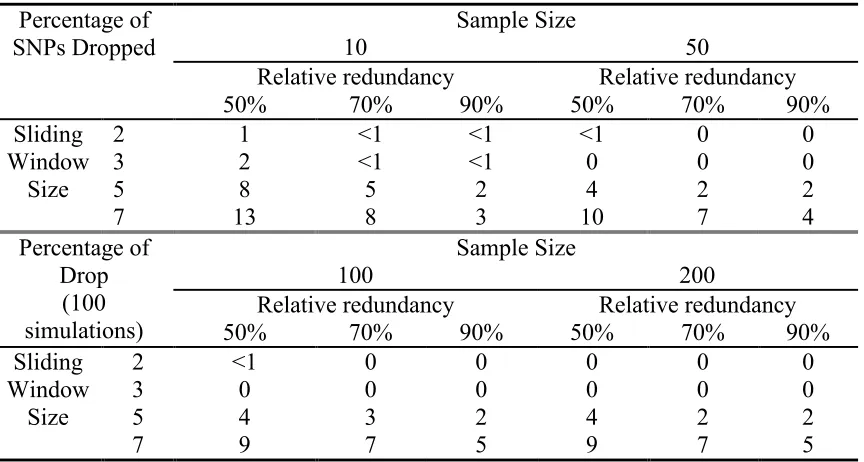
3.3.4.1 Simulation study I: will the SNP selection procedure drop “important” SNPs?………46
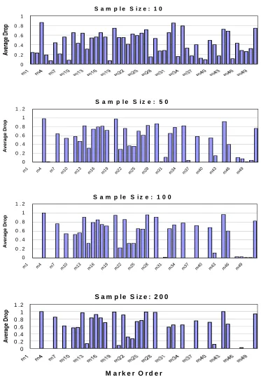
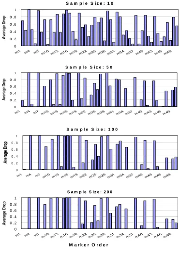
3.3.4.2 Simulation Study II: what sample size is required to ensure consistent results across sample?………..48
3.3.5 Validation Criteria………50
3.3.6 Data Sets……….………..51
3.4 Results………53
3.4.1 Simulation Study I……….……….………..53
3.4.2 Simulation Study II……….………..55
3.4.3 Experimental data results………..57
3.5 Discussion………..60
3.6 Acknowledgement ………66
3.7.1 Obtaining the matrix of pairwise LD for bi-allelic markers……….67
3.7.2 Determining effective/redundant numbers of markers, Le,Lr……….68
3.8 References……….70
3.9 Figure Legends……….……….76
4. A Random Effect Model for Quantitative Trait and Haplotypes Association Test Considering Treatments and Gene-treatment Interactions ………...……….82
4.1 Abstract………..83
4.2 Introduction………85
4.3 Methods ………...………..90
4.3.1 A brief introduction to Model I and II. ………..……..90
4.3.2 Relating the variance components of a QTL and a marker………..92
4.3.3 The random effect model ………95
4.3.4 Hypothesis Testing...……….…………99
4.3.5 Simulation study ………101
4.4 Results………..…………105
4.4.1 Estimated type I error rate. ……….105
4.4.2 Estimated Power ………...105
4.5 Discussion………..………..108
4.6 Acknowledgement………...111
4.7 Appendix………..112
4.8 References………115
viii
List of Tables Page
Table 2.1 Analysis result for isolate replicate 25………..……… 29
Table 2.2 Number (percentage) of replicates correctly identifying each of the 7 major genes… 30
Table 2.3 False positive and true discovery rates over all 50 replicate………….………31
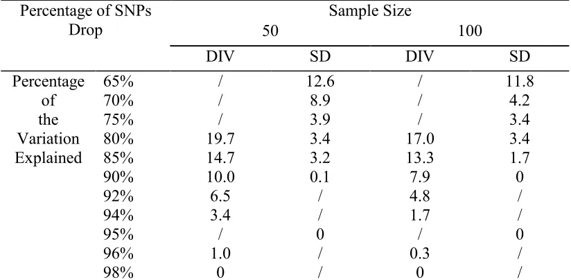
Table 3.1 Percentage of SNPs dropped in LE using SD with variation explained 85% haplotype phase-unknown……….………72
Table 3.2 Percentage of SNPs dropped in LE using DIV with variation explained 92% haplotype phase-unknown……….………73
Table 3.3 Percentage of SNPs dropped in LE using DIV with variation explained 92% haplotype phase-known……….74
Table 3.4 Percentage of SNPs dropped in LE using different variation explained values………75
Table 4.2 Simulation effects when quantitative trait locus (QTL) is from multiple SNP mutations………..121
x
List of Figures Page
Figure 3.1: 50 SNPs’ average drop percentage across 100 simulations on the “high LD” data
when haplotype phase is unknown………78
Figure 3.2: 50 SNPs’ average drop percentage across 100 simulations on the “high LD” data when haplotype phase is unknown………....79
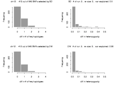
Figure 3.3: Apply SD and DIV on the chromosome 12 region with 649 SNPs………80
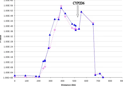
Figure 3.4: Association between CYP2D6 PM phenotype and haplotypes……….………..81
Figure 4.1: Power of drug effects type III tests………...123
Figure 4.2: Power of genetic effects type III tests when the QTL is a single young mutation………...124
Figure 4.3: Power of genetic effects type III tests when the QTL is a single old mutation………...125
Figure 4.5: Power of gene-drug interaction tests when the QTL is a single young mutation………...127
Figure 4.6: Power of gene-drug interaction tests when the QTL is a single old mutation………...128
1
Chapter One
1.1 Complex trait gene mapping
Studying genetic variation, especially mapping human drug response and disease susceptibility
genes, has drawn increasing attention since the near-completion of human genome sequencing
(Venter et al. 2001; Lander et al. 2001). With a lot of fruitful results accomplished since 1913
(Sturtevant 1913), mapping genetic traits remains a hard task. One main reason is that mapping
genes is always like fishing in a sea of large size genomes, such as the human genome consisting
of 3×10⁹ base pairs. Another reason is the complexity of genetic traits such as incomplete
penetrance, genetic heterogeneity, and polygenic inheritance. Due to the development of
technologies and methodologies, the detection can be conducted based on the relations between
inheritance patterns of a trait and chromosome components located by genetic markers, instead
of the knowledge of the gene functions (Nakamura et al. 1987; Lander and Schork 1994). Most
frequently used methods include linkage analysis (including model based and allele sharing
methods), association studies, and experimental crosses.
Linkage analysis methods rely on the assumption that the chromosome region closely linked to
the disease mutation allele tends to be conserved in pedigrees and leads to a certain inheritance
pattern of this chromosome piece among affected individuals. With current genotyping
techniques, linkage analysis is widely applied to genome-wide gene mapping based on several
hundred markers spread across the genome. It has been utilized for a relatively long time and
quite successful in mapping Mendelian diseases (Kerem et al. 1989) and some complex disease
such as Alzheimer’s disease and psoriasis (Pericak-Vance et al. 1991; Tomfohrde et al. 1994).
Model-based linkage analysis methods are believed to be more powerful if the model parameters,
3 results can be misleading if specified parameters do not mimic the reality correctly. On the other
hand, allele-sharing methods are usually non-parametric, more robust, but presumably less
powerful. The success of the linkage analysis in mapping complex human traits is still limited.
Multiple genes with intermediate or small effects are believed to be the genetic basis of the
complex traits. Based on their calculations, Risch and Merikangas (1996) predicted that linkage
analysis would require unrealistic large sample sizes to obtain the statistical power required to
detect relatively medium or small genetic effects comparing to the effects of some Mendelian
diseases, and therefore might not be suitable for mapping complex traits. Several multi-point
linkage analysis methods (Kruglyak et al. 1996; O'Connell 2001) were proposed and presumed
to be more powerful than single-point methods (Penrose 1953; Elston and Stewart 1971).
Obtaining large pedigrees is also considered crucial. However, their further achievements are
still under inspection. Another limitation of linkage analysis is that the size of the detected region
usually extends over more than 1cM (approximately 1000kb in human genome), which might be
too large to pinpoint the targeted trait gene. Narrowing down a linkage region depends on the
number of recombinations in the pedigree, which, in turn, depends on the number of meioses,
pedigree structure and the sample sizes.
Association analysis methods are more “population based’ in a sense that they try to locate the
trait locus of interest by detecting the differences in marker allele frequencies between cases and
matched controls from a population. The marker (markers) showing a significant difference is
assumed to be either the trait locus or in linkage disequilibrium (LD) with it. The length of the
detected region in an association study depends on a sample representing the recombination
much smaller than that from linkage analyses, which depends the patterns within families. It
might vary in different chromosome regions from 1 kb to several hundred kb and from
population to population. Relying on the inheritance pattern of a whole population, association
studies are believed to have more power in mapping complex trait genes with small or
intermediate effects (Jorde 1995). Therefore, they play more and more important roles in
complex trait mapping (Ryder et al. 1979; Martin et al. 2000). Currently, most association
studies are conducted on either candidate genes or pre-identified linkage regions. On the other
hand, genome-wide association studies rely on relatively short distances of LD, and hence are
constrained by the required high marker density, corresponding high genotyping costs and lack
proper analysis methods. However, the fast development of high throughput single nucleotide
polymorphism (SNP) genotyping techniques (Prince and Brookes 2001; Cutler et al. 2001) and
statistical analysis methods are expected to be able to address these problems in the near future.
Utilizing unrelated population case-control samples is a major advantage of the association
studies since the samples are relatively easy to obtain, but also a major limitation. Spurious
associations could be caused by population stratification or recent population admixture (Weiss
1993), and by any markers confounding with trait locus of interest. Furthermore, the effects
might be presented even after a careful matching of cases and controls. Two approaches were
proposed to solve this problem. One relies on within family controls (Spielman et al 1993;
Knapp et al 1993). Within family controls also provide good matches for the environments,
although the concern of losing power due to over-matches of siblings was also raised (Risch and
Teng 1998). The other approach is to develop methods either correcting or detecting
5 Although the possible spurious association is the most frequently raised problem of the
association studies, its effect on false positive findings is still unclear.
Experimental crosses have been also widely applied to genetic trait mapping and have already
made great contributions to the study of human complex diseases like diabetes and obesity
(Forsell et al. 2000; Hamilton-Williams et al. 2001). Although their applicability is limited in
studying certain human genetic traits, experimental crosses are viewed to be powerful and even
the “limit-breaking” tool in future genetic variation studies. These methods have the advantage
of relying on the relative genetic homogeneity of animal or plant models and the ability to study
a relatively large number of animal or plant generations at a time. Therefore, they can be
employed to solve the genetic heterogeneity problem in the complex traits.
Replicating positive findings is essential in proving that the findings are true positives in any
study. Contradicting reports about the same regions or genes are often seen in genetic trait
mapping. One possible reason is false positives in some studies. Another possibility is lack of an
appropriate design in the replicated studies. Therefore, replications need to be carefully selected
to avoid the heterogeneity from the data showing the original positive signal, and large enough to
possess the statistical power of replicating the original signal (Lernmark and Ott J1998). The
biological and experimental proof should be considered critical and might be considered as the
only “real” proof.
1.2 Power comparison of genome wide disease gene mapping strategies.
but usually give resolutions larger than 1cM subject to pedigree structure and sample sizes.
Therefore, association studies are usually conducted to do fine mapping under linkage peak
showing significant signals. Furthermore, linkage analysis might lack statistical power to detect
moderate genetic effects of complex diseases. On the other hand, association tests have the
ability to narrow disease susceptibility regions down to 1-100kb depending on the extent of LD,
and are believed to be more powerful than traditional linkage studies. However, conducting a
genome-wide association study requires a large genotyping effort due to the required high
marker density. These pros and cons of both approaches lead to the question of which of the two
genome-wide gene mapping strategies, applying association tests as a primary approach vs. as a
follow-on to family-based linkage studies, has more power in genome wide studies.
In chapter 2, these two approaches were investigated utilizing GAW12 simulated data and
methodologies suitable for the pedigree structure under study. Furthermore, a strategy of using
Simes test (Simes 1986) as a method for combining results from LD tests of adjacent markers
was investigated in order to control false positives. The results showed that the genome-wide
association based tests are much more likely to identify genes, although a denser map of markers
is required. The results were published. (Meng Z, Zaykin DV, Karnoub MC, Sreekumar GP, St
Jean PL, Ehm MG. “Identifying susceptibility genes using linkage and linkage disequilibrium
analysis in large pedigrees.” Genet Epidemiol. 2001; 21 Suppl 1:S453-8.)
1.3 LD structure study and marker selection for association studies
One limitation of the association studies is the high genotyping cost due to the required high
7 marker densities is to increase the chance of either including disease susceptibility loci or
markers in LD with them and to provide enough statistical power to detect them. The current
development of high-density maps of Single Nucleotide Polymorphisms (SNPs) provides a great
source for such markers. However, genotyping of closely spaced SNPs frequently yields highly
correlated data due to extensive LD between markers, it might be considered as “wasting
resources” when these markers don’t yield significantly different information in association
studies.
Several recent studies investigated the empirical LD structure on different human chromosomal
regions, and discovered that LD appears to be organized in block-like structures. Within these
“blocks”, limited genetic variation was observed. Daly et al. (2001) analyzed 516 chromosomes
from a European-derived population typed for 103 SNPs in a 500 kb region on chromosome
5q31, and found the region could be decomposed into discrete haplotype blocks, which spanned
up to 100 kb and contained 5 or more common SNPs. Johnson et al. (2001) scanned 135 kb of
DNA, genotyped 122 markers in 9 genes, and determined haplotypes in a minimum of 384
European individuals. They advocated determining haplotypes as an approach that would
provide the relationships between all alleles in the region. Based on all these observations,
researchers raised a possibility of developing the “haplotype map” for human, which is a map
consisting of haplotype blocks and SNPs in relatively low LD linking between blocks. Because
of the low genetic diversities within blocks, only a relatively small number of SNPs is required
to retain most of the information. Therefore, the association studies can provide a much clearer
picture by conducting analyses based on haplotype blocks and much lower cost for genotyping.
simulation results showing that the required SNP number might be much larger (Kruglyak 1999).
The future of the haplotype map is still unknown, and its impact on association studies still
requires further investigation.
Regardless of these contradictory views, using LD or haplotype information to select a subset of
SNPs that optimizes the information retained in a genomic region while reducing the genotyping
cost and simplifying the analysis without relying on “haplotype blocks” is still possible and can
be quite helpful in association studies. In chapter 3, two procedures are developed to achieve this
goal. One utilizes a spectral decomposition method based on matrices of pair-wise LD between
markers, and the other extends David Clayton’s htSNP selection method. The procedures require
genotype information for a large initial set of SNPs on a small number of samples to select an
optimum subset of SNPs that could be efficiently genotyped on larger numbers of samples while
retaining most of the information on genetic variation. The properties of these procedures were
studied using simulated data sets; minimum sample sizes needed for achieving consistent results
were recommended; the procedure performances were evaluated using experimental data sets
with measures of haplotype information; the possible impact of the marker selection on the
association study was illustrated using a real example.
1.4 Mixed model for association study considering drug and gene-drug
interaction
Investigating genetic effects and gene×treatment interactions is essential in determining
individual differences in drug responses, a long desired problem in clinical trial studies. With this
9 right treatment to the right person. In order to study how genes are related to efficacy and safety
of a medicine, multiple markers are genotyped in candidate genes on samples collected in
clinical trials. Challenges for analysis include lack of validated statistical genetic methods,
multiple correlated genetic markers, and low sample sizes. Quantitative response traits are of
interest because they better reflect drug pharmacokinetics and pharmacodynamics, therefore
provide more information on drug responses. Models taking into account the nature of genetic
data including allelic, genotypic and haplotype effects are critical to extracting maximum
information.
A linear regression approach considering genetic, treatment effects and their interactions directly
should address this problem well. However, further studies are needed to understand the effects
of the multiple factors involved, such as the nature of genetic effects, gene-drug interactions, and
marker spacing in candidate genes, since the testing powers of different models, and “the best”
approach vary under those effects. Therefore, in chapter 4, a model is proposed to separate the
genetic effect into haplotype allelic additive effects and dominant effects of multiple markers in
the candidate genes (Weir and Cockerham 1977; Zaykin et al. 2002), model the treatment,
haplotypes additive effects, and treatment-haplotype interactions, and relate these effects to a
quantitative trait. Furthermore, the variance components of a marker locus were related to those
of a functional trait locus through genetic effects of trait alleles, LD between trait locus and
markers, as well as their allele frequencies. Therefore, randomly genotyping markers in the
candidate genes or regions of interests will introduce uncertainty into the study when the typed
markers are not functional sites in question. Hence, more appropriate statistical models are
interactions as random to account for this uncertainty. The model is compared to an analysis of
variance approach with single marker genotypic classes and haplotype effects treated as fixed
effects, and the power of utilizing multiple markers with a haplotype approach versus single
11
Reference
Cutler DJ, Zwick ME, Carrasquillo MM, Yohn CT, Tobin KP, Kashuk C, Mathews DJ, Shah
NA, Eichler EE, Warrington JA, Chakravarti A (2001) High-throughput variation
detection and genotyping using microarrays. Genome Res 11(11):1913-25
Devlin B and Roeder K (1999) Genomic Control for Association Studies. Biometrics
55:997-1004
Elston RC and Stewart J (1971) A general model for the analysis of pedigree data. Hum Hered
21:523-542.
Forsell PA, Boie Y, Montalibet J, Collins S, Kennedy BP (2000) Genomic characterization of the
human and mouse protein tyrosine phosphatase-1B genes. Gene 260:145-53
Hamilton-Williams EE, Serreze DV, Charlton B, Johnson EA, Marron MP, Mullbacher A,
Slattery RM (2001) Transgenic rescue implicates beta2-microglobulin as a diabetes
susceptibility gene in nonobese diabetic (NOD) mice. PNAS 98(20):11533-8
Jorde LB (1995) Linkage disequilibrium as a gene-mapping tool. Am J Hum Genet 56:11-14
Kerem B, Rommens JM, Buchanan JA, Markiewicz D, Cox TK, Chakravarti A, Buchwald M,
Tsui LC (1989) Identification of the cystic fibrosis gene: genetic analysis. Science
245:1073-80
Knapp M, Seuchter SA, Baur MP (1993) The haplotype-relative risk (HRR) method for analysis
of association in nuclear families. Am J Hum Genet 52:1085-1093
Kruglyak L. (1999) Prospects for whole-genome linkage disequilibrium mapping of common
disease genes. Nat Genet 22:139-44
Lander ES, Linton LM (2001) Initial sequencing and analysis of the human genome. Nature
409:860-921
Lernmark A and Ott J. (1998) Sometimes it's hot, sometimes it's not. Nat Genet 19:213-214
Kruglyak L, Daly MJ, Reeve-Daly M, Lander ES (1996) Parametric and non-parametric linkage
analysis: a unified multipoint approach. Am J of Hum Genet 58:1347-1363
Martin ER, Gilbert JR, Lai EH, Riley J, Rogala AR, Slotterbeck BD, Sipe CA, Grubber JM,
Warren LL, Conneally PM, Saunders AM, Schmechel DE, Purvis I, Pericak-Vance MA,
Roses AD, Vance JM. (2000) Analysis of association at single nucleotide polymorphisms
in the APOE region. Genomics 63:7-12
Nakamura Y, Leppert M, O'Connell P, Wolff R, Holm T, Culver M, Martin C, Fujimoto E, Hoff
M, Kumlin E, et al. (1987) Variable number of tandem repeat (VNTR) markers for
human gene mapping. Science 235:1616-22
O'Connell JR. (2001) Rapid multipoint linkage analysis via inheritance vectors in the
Elston-Stewart algorithm. Hum Hered 51:226-240.
Pericak-Vance MA, Bebout JL, Gaskell PC Jr, Yamaoka LH, Hung WY, Alberts MJ, Walker
AP, Bartlett RJ, Haynes CA, Welsh KA, et al. (1991) Linkage studies in familial
Alzheimer disease: evidence for chromosome 19 linkage. Am J Hum Genet. 48:1034-50
Penrose LS. (1953) The general purpose sib-pair linkage test. Annals of Eugenics (London). 18,
120-124
Pritchard JK and Rosenberg NA. (1999) Use of Unlinked Genetic Markers to Detected
Population Stratification in Association Studies. Am. J. Hum. Genet. 65:220-228
Pritchard JK, et al. (2000) Inference of Population Structure Using Multilocus Genotype Data.
13 Prince JA, Brookes AJ Towards high-throughput genotyping of SNPs by dynamic allele-specific
hybridization Expert Rev Mol Diagn (2001) 1:352-358
Risch N, Teng J (1998) The relative power of family-based and case-control designs for linkage
disequilibrium studies of complex human diseases I. DNA pooling. Genome Res
8:1273-88
Ryder LP, Christy M, Nerup J, Platz P, Svejgaard A, Thomsen M (1979) HLA studies in
diabetics. Adv Exp Med Biol 119:41-8
Simes RJ (1986): An improved Bonferroni procedure for multiple tests of significance.
Biometrika 73:751-754.
Spielman RS, McGinnis RE, Ewens WJ (1993) The transmission test for linkage disequilibrium:
the insulin gene and insulin-dependent diabetes mellitus (IDDM). Am J Hum Genet
52:506-516
Sturtevant AH (1913) J.EXP. Zool. 14, 43
Tomfohrde J, Silverman A, Barnes R, Fernandez-Vina MA, Young M, Lory D, Morris L,
Wuepper KD, Stastny P, Menter A, et al. (1994) Gene for familial psoriasis susceptibility
mapped to the distal end of human chromosome 17q. Science 264:1141-5
Venter JC, et. al. (2001) The sequence of the human genome. Science 291:1304-1351
Weir BS and Cockerham CC (1977): Two-locus theory in quantitative genetics. In: Proceedings
of the international Conference on Quantitative Genetics, (eds) Pollak E, Kempthorne O,
Bailey TB, Iowa State University Press, Ames, Iowa, pp 247-269
Zaykin DV, Westfall PH, Young SS, Karnoub MA, Wagner MJ, Ehm MG. (2002) Testing
Association of Statistically Inferred Haplotypes with Discrete and Continuous Traits in
15
Chapter 2
Identifying Susceptibility Genes Using
Linkage and Linkage Disequilibrium
SUMMARY
Linkage and linkage disequilibrium tests are powerful tools for mapping complex disease genes.
We investigated two approaches to identifying markers associated with disease. One method
applied linkage analysis and then linkage disequilibrium tests to markers within linked regions.
The other method looked for linkage disequilibrium with disease using all markers. Additionally,
we investigated using Simes test to combine p-values from linkage disequilibrium tests for
nearby markers. We applied both approaches to all replicates of the GAW12 problem 2 isolated
population data set. We reported results from the 25th replicate as if it were a real problem and
assessed the power of our methods using all replicates. Using all replicates, we found that testing
all markers for linkage disequilibrium with disease was more powerful than identifying markers
that were in linkage with disease and then testing markers within those regions for linkage
disequilibrium with the implementations that we chose. Using Simes test to combine p-values for
17
INTRODUCTION
In this paper, we aim to compare the strategies of identifying markers in linkage
disequilibrium within regions linked to disease versus identifying markers in linkage
disequilibrium across the genome. Furthermore, we investigate the strategy of using Simes test
as a method for combining results from linkage disequilibrium tests for nearby markers. We
analyzed GAW12 simulated data using one linkage analysis method (SimIBD) applied to a
10cM map of markers to identify broad regions likely to contain disease genes and then one
linkage disequilibrium analysis method (PDT) applied to all markers within those regions. We
compared the results to applying another LD analysis method (Transmit) on all markers. We
investigated use of the Simes test to combine results from linkage disequilibrium tests for
adjacent markers. We feel that these are reasonable approaches for identifying markers nearest to
disease genes without an abundance of false positives.
The present study was completed on all the replicates of the isolated population for
GAW12 problem 2. We investigated the affection status trait provided to search for disease
susceptibility genes. To illustrate our approaches, we report the results for the 25th replicate. We estimated the power to find each of the 7 genes for a preset equal false positive rate for both
approaches. The GAW12 problem 2 data set included 2855 STR markers with an average
METHODS
We selected a single-point linkage analysis method, SimIBD [Davis, et al., 1996], to
investigate linkage of the affection status trait with genetic makers. This method was selected for
its speed and ability to analyze large pedigrees. SimIBD presents a non-parametric
simulation-based statistic, which measures identity by descent sharing of alleles between affected relative
pairs, reports a normalized Z statistic, weighted using population allele frequencies and gives a
conditional empirical p-value. An empirical null distribution is determined by simulating marker
genotypes in the affected subjects conditional on the marker genotypes in the unaffected
subjects. The p-value reported is determined by the proportion of points in the null distribution
that has a Z value greater than the observed Z statistic. To imitate a genome scan approach, we
selected one marker every 10cM for analysis. We thought that it was a reasonable approach
since, for micro-satellite makers, adding markers at a finer density isn’t likely to increase the
information available for linkage: linkage usually extends more than 10cM. We defined a linkage
region as significant if the p value at a peak was less than 0.05. The region started from the first
marker with a p value greater than 0.17 (Lod score = 0.2) to the left of the peak to the first
marker with a p value greater than 0.17 to the right of the peak.
To identify markers in linkage disequilibrium with disease within linkage regions, we
applied the transmission disequilibrium test [Spielman, et al., 1993] using the PDT program
[Martin et al., 2000]. PDT uses data from affected and unaffected individuals in related nuclear
families in extended pedigrees. It calculates a statistic, T, which sums weighted transmission
19 hypothesis of no association in the presence of linkage, this statistic is asymptotically normal
with mean 0 and variance 1. When investigating age of onset and age of exam, we noted that
many of the individuals identified as unaffected were examined at ages that were considerably
less than the mean age of onset. We suspected that some people classified as unaffected should
have been called unknown, because they were too young to develop the disease. By investigating
the distributions for age of onset in affected people and age of exam in unaffected people, we
decided that individuals needed to be at least 45 years at exam to be identified as unaffected with
disease. Individuals less than 45 years at exam and not affected, were assigned an unknown
affection status. Then we calculated the above statistic using the new affection status. The
p-values reported were based on the normal distribution.
We applied the transmission disequilibrium test using Transmit [Clayton D, 1999] to test
for linkage and association using all the markers, not just ones within linkage regions. This
method calculates a score test based on a partial score function that omits the terms most
influenced by hidden population stratification. The test is proposed for the situation in which
transmission is uncertain and is applied to all nuclear families within the extended families.
Under the null hypothesis of no linkage or association, the score vector asymptotically follows a
χ2 distribution with degrees of freedom (df) equal to
H-1 where H is the number of distinct
alleles. The reported statistic uses transmission information only to affected individuals. It has
been shown [Clayton D, 1999] that the Transmit statistic is still valid while using all the affected
siblings, even when you are assuming linkage. However, linkage induces a correlation structure
within distant pedigree members that is not taken into account in the implementation of Transmit
Transmit statistic, we tested the null hypothesis of no linkage and no association. This is distinct
from the PDTest, which is a valid test for association in the presence of linkage. Because the
Transmit test requires the assumption of Hardy-Weinberg equilibrium, we tested each marker to
see if the genotype frequencies were in HWE.
To identify significant regions of linkage disequilibrium based on statistics calculated
with correlated markers, we applied Simes test [Simes, RJ 1986], which is a method for testing
the intersection of hypotheses and controlling type 1 error for the whole set. Sarkar and Chang
[1997] proved that it was applicable to positively correlated dependent hypotheses. Simes test
reports a combined p-value for a set of p-values based on the following formula, where p[i] is the
ith order statistic and n is the number of p-values in the set.
] ] [ , ] 1 [ 1 ,..., ] 3 [ 3 , ] 2 [ 2 , ] 1 [ [ n p n p n n p n p n np Min − −
We applied Simes test replacing the p-value of the middle marker by the combined p-value from
the first n markers starting from the p-ter of the chromosome. Note that this would control the
type 1 error rate of only the n markers, if we had one fixed. However, we are using this method
as a smoothing technique for highly variable p-values. We continued this for each set of n
markers in a sliding window across the chromosome. To determine the window size, we
calculated the correlation of the marker p-values for the PDT and the Transmit results. The size
of the window remained constant for each method. We assumed that the markers were equally
spaced and the autocorrelation depended only on the number of markers between the two
21 We analyzed all 50 replicates using these 4 methods (1-SimIBD & PDT, 2-Transmit,
3-SimIBD, PDT with Simes, and 4-Transmit with Simes). When comparing the markers with
significant linkage disequilibrium tests to the “Answers”, any marker was a true positive if it was
3 cM either to the left or to the right of the disease gene. Applying SimIBD and PDT tests
sequentially to the data made it difficult to control the type I error for each approach. Applying
Simes test complicated this further. To make the comparison of these 4 methods fair, we adjusted
the α level used for each test within each approach so that the observed false positive rate, for the
approach, was close to 0.05.
The observed false positive rate was calculated as the proportion of all markers tested
identified as significant that were not within 3cM of a gene. We summarized the number of times
we identified each major gene in 50 replicates and computed the true discovery rate (the number
RESULTS
We didn’t find any evidence against the HWE assumption. The p-values of linkage
disequilibrium analysis results (PDT and Transmit) were positively correlated and the average
correlation extended to 3 markers. We smoothed the PDT and the Transmit results using Simes
test with window sizes of 3.
Replicate 25
We controlled the false positive rate to be 0.05 for all approaches by choosing a different
α-level for each test as follows: when applying Simes test, the α−level was 0.05 for SimIBD,
0.09 for PDT and 0.03 for Transmit. Without Simes test, the α-level was 0.05 for SimIBD, 0.07
for PDT, and 0.05 for Transmit. The results are summarized in Table 1. For each linkage region,
we listed the boundaries of the region and the peak marker name along with the corresponding
p-values. For each set of markers showing significant linkage disequilibrium, we listed p-values
only. Analysis using Transmit resulted in so many significant results that, we listed only the first
12 most significant ones.
We identified 12 linkage regions and 4 LD regions under the linkage regions (SimIBD &
PDT). Among them, the region D09G120-122 contains MG3. The true discovery rate for regions
was 25.0% (1/4) considering 4 regions identified by PDT. Transmit identified 41 LD regions
23 contains MG6 & MG7 and the region D19G026-032 contains MG1. The true discovery rate was
4.9% (2/41).
Power Study
We counted the number of times each major gene was found in the 50 replicates, and
summarized the results in Table 2. We also listed the average number of tests applied, the true
discovery rate and the false positive rate for each approach.
Comparing the SimIBD & PDT approach to the Transmit approach, we can see that a
genome-wide association test did increase our chances of finding the disease genes. Applying
Simes test reduced our power to locate disease genes, but a greater percentage of the markers we
DISCUSSION
We analyzed GAW12 simulated data to compare the two commonly used strategies of
identifying disease genes (linkage disequilibrium analyses within regions linked to disease and
linkage disequilibrium analyses across the genome). Neither of these two approaches was
extremely powerful, but our results show that genome wide linkage disequilibrium analyses
increase the chance of finding genes compared to the linkage and association strategy. The above
conclusion is only based on the implementations we chose in this paper. A possible shortcoming
is that the number of markers to be typed will be significantly higher, but the probability of
finding the genes using any replicate is also much higher with in this approach. Our approach of
using Simes’ test for smoothing p-values is similar in spirit to the method of Goldin, et al.,
[1999] who suggested that p-values could be averaged across certain genetic distances. The
underlying idea of such approaches is that multiple significant results in a chromosomal region
provide more support for the presence of a gene than a single significant result. Thus, the false
discovery rate might be decreased. For similar reason, Juo, et al., [1997] required that the
p-values for flanking markers around significant tests must also show the tendency to be “small”, if
not significant. Terwilliger, et al., [1997] and Knapp [1998] presented theoretical considerations
pointing out that the positive correlation between test statistic values extends further around true
positives. We have chosen Simes’ test based on preliminary simulation study (data not shown)
that revealed its better performance. Both approaches (averaging and applying Simes’ test)
however suffer from the fact that the resulting overall p-value cannot possibly be smaller than
the minimum p-value in the window. As a consequence, the power can be reduced, and Table 2
25 increased. During analysis of GAW12 simulated data sets, Hardy et al. (personal
communication) used another method proposed by Zaykin, et al., [2001] that may not suffer
from the mentioned potential loss of power, allowing the overall p-value to be smaller than the
minimum in the combined set. Further study is needed to compare suggested techniques. Both,
original and smoothed sets of significant results show that the genome-wide association based
tests (i.e. Transmit) are much more likely to identify genes, although a denser map of markers is
ACKNOWLEDGMENTS
Thanks to Xiaobin Li, Xiaohui Luo, Brad Freeman, Santhi Sampath, and Rusty Czerwinski for
27
REFERENCES
Clayton D (1999): A generalization of the transmission/disequilibrium test for
uncertain-haplotype transmission. Am. J. Hum. Genet 65: 1170-1177.
Cottingham RW Jr, Idury RM, Schaffer AA (1993): Faster sequential genetic linkage
computations. Am. J. Hum. Gent. 53: 252-263.
Davis S, Schroder M, Goldin LR, Weeks DE (1996): Non-parametric simulation-based statistics
for detecting linkage in general pedigrees. Am. J. Hum. Genet. 58: 867-880.
Goldin LR, Chase GA, Wilson AF (1999): Regional inference with averaged p-values increases
the power to detect linkage. Genetic Epidemiology 17:157-164.
Juo SH, Beaty TH, Duffy DL, Maestri NE, Prenger VL, Zeiger J, Lei HH, Coresh J (1997): A
comprehensive analysis of complex traits in problem 2A. Genetic Epidemiology 14(S):815-820.
Knapp M (1998): Discriminating between true and false-positive peaks in a genomewide linkage
scan, by use of the peak length. Am. J. Hum. Genetics. 62:1561-1562.
Martin ER, Monks SA, Warren LL, Kaplan NL (2000): A test for linkage and association in
Ott J (1989): Computer-simulation methods in human linkage analysis. Proc. Natl. Acad. Sci.
USA 86(11):4175-8
Sarkar SK, Chang CK (1997): The Simes method for multiple hypothesis testing with positively
dependent test statistics. J. Am. Stat. Assoc. 92, 1601-1608.
Simes RJ (1986): An improved Bonferroni procedure for multiple tests of significance.
Biometrika 73:751-754.
Spielman RS, McGinnis RE, Ewens WJ (1993): Transmission test for linkage disequilibrium: the
insulin-dependent diabetes mellitus. Am. J. Hum. Genet. 52: 506-516.
Terwilliger JD, Shannon WD, Lathrop GM, Nolan JP, Goldin LR, Chase GA, Weeks DE (1997):
True and false positive peaks in genomewide scans: applications of length-biased sampling to
genome mapping. Am. J. Hum. Genet. 61:430-438.
Weeks DE, Ott J, Lathrop GM (1990): SLINK: a general simulation program for linkage
analysis. Am. J. Hum. Genet. 47: A204
Zaykin DV, Zhivotovsky LA, Westfall PH, Weir BS (2001): Truncated product method for
29 Table 2.1 Analysis result for isolate replicate 25
SimIBD SimIBD & PDT with
Simes
Transmit with Simes
Linkage regions
Marker & p-value at peak
LD regions
p value at peak
LD regions p-value at
peak D01G115
-143
D01G120 & 0.0061
D01G050-052 0.0009
D02G167 -186
D02G177 & 0.0241
D01G126-128 0.0045
D03G010 -057 D03G023 & 0.0037 D03G024-026
0.0858 D03G043-045 0.0001
D03G057 -073
D03G065 & 0.0208
D04G153-155 0.0015
D04G010
-032 D04G026 & 0.0214 D05G045-050 0.0012
D05G112 -142
D05G132 & 0.0089
D06G032-043* 0.0003
D06G085 -119
D06G097 & 0.0472
D06G055-057 0.0024
D06G129 -152 D06G146 & 0.0257 D06G142-144
0.0303 D08G055-071 0.0018
D09G102 -129 D09G110 & 0.0197 D09G120-122*
0.0432 D12G050-052 0.0021
D18G086
-106 D18G103 & 0.0091 D13G073-075 0.0001
D19G102 -105
D19G105 & 0.0130
D16G107 0.0030
D22G010 -026 D22G016 & 0.0169 D22G024-026
Table 2.2 Number (percentage) of replicates correctly identifying each of the 7 major genes
With Simes Without Simes
Major Gene
Linkage & PDT
Transmit Linkage &
PDT
Transmit
MG1 3 ( 6%) 4 ( 8%) 1 ( 2%) 8 (16%)
MG2 0 ( 0%) 5 (10%) 1 ( 2%) 14 (28%)
MG3 1 ( 2%) 4 ( 8%) 1 ( 2%) 14 (28%)
MG4 0 ( 0%) 4 ( 8%) 0 ( 0%) 10 (20%)
MG5 1 ( 2%) 7 (14%) 2 ( 4%) 12 (24%)
MG6 8 (16%) 44 (88%) 10 (20%) 49 (98%)
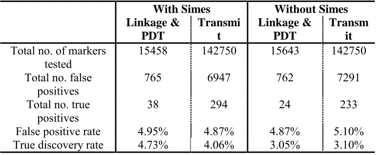
31 Table 2.3 False positive and true discovery rates over all 50 replicates
With Simes Without Simes
Linkage & PDT
Transmi t
Linkage & PDT
Transm it Total no. of markers
tested
15458 142750 15643 142750
Total no. false
positives 765 6947 762 7291
Total no. true positives
38 294 24 233
False positive rate 4.95% 4.87% 4.87% 5.10%
Chapter 3
Selecting Genetic Markers for Association
33
Abstract
Genotyping closely spaced SNP markers frequently yields highly correlated data due to
extensive linkage disequilibrium (LD) between markers. The extent of LD varies widely across
the genome, and drives the number of frequent haplotypes observed in small regions. Several
studies have illustrated that it may be possible to use LD or haplotype data to select a subset of
SNPs that optimizes the information retained in a genomic region while reducing the genotyping
cost and simplifying the analysis. Generally applicable methods are needed to select a minimum
subset of SNPs sufficiently retaining most information provided by haplotypes observed in a
region. We proposed a spectral decomposition method based on the matrices of pairwise LD
between markers, modified David Clayton’s htSNP selection method that utilizes haplotype
information, and proposed algorithms allowing the methods to be applied to large chromosomal
regions. Our procedures require genotype information for a large initial set of SNPs on a small
number of individuals, and select an optimum subset of SNPs that could be efficiently genotyped
on larger numbers of samples while retaining most of the genetic variation in samples. We
studied the properties of procedures using simulated data sets in linkage equilibrium and
disequilibrium, and reported minimum sample sizes needed for consistent results. Procedures
were applied to experimental data sets with SNPs at average densities of one SNP every 20 or 30
kb and evaluated using haplotype information measures. Both procedures were similarly
effective at reducing the genotyping requirement while maintaining the genetic information
content throughout the regions. We also illustrated the procedure impact on an association study
result in a region around the CYP2D6 gene (Hosking et al. 2002).
Introduction
Efforts to positionally clone susceptibility genes for common, oligogenic diseases have led to the
development of high-density maps of Single Nucleotide Polymorphisms (SNPs) distributed
across the human genome (Sachidanandam et al. 2001). Theoretical studies have suggested that
association tests employing such high-density SNP maps, either as a primary approach or as a
follow-on to family-based linkage studies, should be more powerful in detecting disease
susceptibility genes than traditional linkage approaches (Risch and Merikangas 1996). However,
the precise numerical meaning of “high-density” is a matter of debate, and has significant
implications on the cost and practicality of conducting SNP association studies. An optimum
strategy would be to genotype enough SNPs to capture the large majority of information on
genetic variation within a defined chromosomal region while avoiding typing SNPs that yield
redundant information due to extensive linkage disequilibrium (LD) between nearby SNPs.
Defining the optimum set of SNPs will require knowledge of the patterns of linkage
disequilibrium across the human genome.
Recently, several studies investigated the empirical LD structure on different human
chromosomal regions, and discovered a common pattern that LD appears to be organized in
block-like structures, where a contiguous group of SNPs comprising a block show high levels of
pair-wise LD between SNPs and where there is little LD between SNPs in different blocks.
Authors (Subrahmanyan et al. 2001; Daly et al. 2001; Johnson et al. 2001; Dawson et al. 2002;
Gabriel et al. 2002; Patil et al. 2001) have reported block-like LD structures showing
considerable spatial variation across different genomic regions, extending up to several hundred
35 haplotype diversities within blocks, given the number of SNPs involved, are observed not only in
genotype data with numerically inferred haplotypes, but also in experimentally determined
haplotype data (Patil et al. 2001). The reduction of haplotype diversities suggests the possibility
of identifying SNPs to define the common haplotypes thereby reducing the number of markers
needed to capture the majority of the genetic information about the region. A procedure that
utilizes genotype information on a small number of samples to prioritize SNPs for typing on a
large number of samples could be useful in increasing the experimental efficiency in any project
involving a high-density map of SNPs. Examples include testing multiple SNPs within a
candidate gene for association, fine-mapping a region identified using linkage analysis, and
testing thousands of SNPs as part of a genome-wide association study. Furthermore using a
technique to identify the most independent and informative SNPs could be helpful in interpreting
analyses across a region where a large number of highly correlated SNPs have been typed. Such
a procedure could helping an analyst see real support for the association in a region without the
redundant information provided by highly correlated SNPs. On the other hand, any “marker
selection procedure” relies on an arguable assumption that common SNP variation can provide
high predictive values for risks associated with complex diseases (Couzin 2002). Thus, these
procedures are only valuable to the extent that the original set of SNPs is useful for association
mapping purposes. Nevertheless, marker selection can be viewed as a procedure for identifying
polymorphisms most characteristic of underlying populations.
Several algorithms have been proposed to detect haplotype blocks and (or) select markers. Patil
et al (2001) utilized a greedy algorithm to partition the entire chromosome into a set of
distinguish at least α percent of the unambiguous haplotypes in each block. Zhang et al (2002)
extend Patil et al’s greedy algorithm to a dynamic programming algorithm, which can guarantee
an optimal solution for haplotype partitioning. Therefore, both Patil et al and Zhang et al selected
markers by identifying the minimum number of SNPs distinguishing at least α percent of the
unambiguous haplotype in the blocks. These algorithms require haplotype phase known data. In
this case, haplotypes were determined experimentally. These procedures are not applicable to
unphased genotype data, and rely on their definitions of block boundaries to select markers.
Other “block defining” algorithms such as those described in Daly et al (2002) and Gabriel et al
(2002) do not require phase known haplotype data. Daly et al used a combination of methods
including familial data and the EM algorithm to estimate haplotype frequencies. Then they
initially defined blocks by comparing the observed haplotype heterozygosity with that expected
assuming Hardy Weinberg Equilibrium within consecutive five markers windows, identifying
“lower diversity haplotypes cores”, and constructing “blocks” by extending or shrinking two
ends of the cores until reaching the longest local minimum “blocks”. Next, a hidden Markov
model was also used to formally define the blocks by assigning observed chromosomes to one of
the four ancestral haplotypes, accessing the significance of the estimations of the historical
recombination rate (θ) between each pair of markers. Gabriel et al used D’ and associated
confidence intervals as a measure of the historical recombination and defined “blocks”. Both
methods appear to be specific for the particular data sets used and their general applicability is
not known. Johnson et al (2001) proposed two methods to select markers within genes based on
gene haplotypes constructed either using the family data or the expectation-maximization (EM)
algorithm on unrelated individuals. One method orders the haplotypes by their similarities and
37 Clayton (2001) to select haplotype tagging SNPs (htSNPs) to best extract the haplotype
information in a gene. The first method is difficult to automate, and the second can become quite
computationally intensive when a large number of markers are considered in a region. (Detailed
reason is shown later.) Both methods require the predetermination of haplotypes for the region
considered, which is difficult when the region contains a large number of markers.
It is worth noticing that all the “block detecting” methods mentioned may result in differing
block boundaries. Given the diversity of methods used to define blocks and conflicting assertions
as to whether they exist at all (Couzin 2002), we choose to develope marker selection procedures
that do not rely on defining “blocks”. Instead, we select a set of SNPs that retain haplotype
information similar to an original (and presumably) larger set of SNPs. Furthermore, the
procedure should be applicable to regions with a large number of SNPs, and data sets without
haplotype phase information or family information. We propose a method based on the spectral
decomposition of the matrix of the pair-wise linkage disequilibrium coefficients of the markers,
and compare it to the htSNP diversity method proposed by Clayton (2001). Both methods can be
utilized to select a subset of markers that maintain haplotype information available from the set
of markers before selection. The spectral decomposition of the LD matrix is a reductionist
approach, which considers many pair-wise LD coefficients at one time. Clayton’s htSNP
method relies on haplotype information rather than pairwise LD coefficients making it a
complementary approach. The spectral decomposition method has a population-genetics
justification and advantages over considering a single pair-wise LD coefficient at a time. In
addition, we propose a procedure summarizing the information obtained from a sliding window
local in that they are applied to genetically proximal sets of markers by considering relatively
short windows of markers covering genetic distances that are generally less than 500 kb.
Furthermore, none of the existing marker selection methods have been evaluated using
quantitative criteria describing the proportion of the information retained in the selected marker
sets. We compare two local haplotype diversity measures: the haplotype heterozygosity and the
number of frequent haplotypes before and after application of the procedures to access the
information retained and measure the success of these procedures. We summarize the results
from two simulation studies to evaluate the performance of these procedures, apply them to two
experimental data sets as examples, and also apply them to markers typed around CYP2D6
where an association has been identified to show how the marker selection procedures impact
39
Materials and Methods
We describe two marker selection methods, the procedure extending them to a large
chromosomal region, two simulation studies to evaluate the procedures, and criteria by which we
evaluate the performance of the procedures when applied to two experimental data sets. Our
selection procedures study relatively polymorphic SNPs with minor allele frequency (MAF) of at
least 0.05.
Spectral decomposition (spD)
Population genetics theory predicts that the linkage disequilibrium associated with alleles from
three or more markers decays more rapidly than LD associated with alleles from two markers
(Bennet 1954). Therefore, it is reasonable to describe dependencies between markers by
considering only pairwise correlations. Moreover, the precision of estimates and power to detect
LD associated with alleles from three or more markers quickly diminishes with their order. The
essence of spectral decomposition is to represent an entire variance-covariance matrix (LD
matrix in our case) in terms of its eigenvalues and eigenvectors. Since the spectral
decomposition-based method (spD) that we propose takes into account all pairwise disequilibria
for a set of markers, it assumes that the LD associated with alleles from three or more markers is
negligible. Therefore, the method assumes that most of the practically available haplotype
information can be recovered from pairwise LD and single marker characteristics. Spectral
decomposition is also the basis for the principal component analysis (PCA). In PCA, the sample
variation is represented by a few linear combinations (the eigenvectors) of all original variables
(i.e. SNPs), taken with different weights (the eigenvalues) to reflect their importance. In contrast,
(the importance of the corresponding combinations), and retain only a subset of the original
variables that contribute more to the more important weights. Note that this procedure allows us
to consider the pairwise LD coefficients of all markers at once instead of only considering the
LD measure for a pair of markers at a time. Let L be the number of markers evaluated. For a set
of markers, m1, …, mL, the LD matrix is RLxL with the pair-wise correlation rijas components,
where ∆ij is the composite LD (Weir 1996) between markers i and j. (See Appendix 1)
Applying the spectral decomposition technique, R can be written as
where ei and λi are eigenvectors and eigenvalues of R, i = 1, …,L, and λ1≥ λ2 … ≥λL. Note
that the variables (markers) that contribute more to the eigenvectors associated with the first
several large eigenvalues, are considered the more influential variables (markers) for that LD
matrix, R. Variables that contribute more to the eigenvectors associated with subsequent
eigenvalues, are considered less influential.
To determine if there are variables or markers, which have little or no influence on the LD
matrix, the following Lr index is calculated (See Appendix 2):
T i i L i ie e
R =
∑
=1λ1 )
( 2
2
− =
∑
∑
i i r LL
λ λ
) ˆ var( / ˆ
ij ij
ij
41 Lr equal to 0 indicates that all the markers in the set provide important information and the whole
set should be kept. This measure is derived by examining the conditions of extreme
disequilibrium and complete independence. We find it useful in identifying when no SNPs
should be eliminated from the set. If Lr > 0, the actual number of markers to be retained, x, is
most precisely determined from the inequality:
where α is the proportion of information retained (proportion of variation explained). Therefore,
we retain markers while the sum of the eigenvalues corresponding to the eigenvectors they
contribute more is a high proportion of the sum of all eigenvalues. Appropriate levels for α will
be investigated in the simulation studies.
It is not always clear which marker contributes more to which eigenvalue or eigenvector. To
sharpen marker loadings to particular eigenvectors, we apply the varimax-rotation procedure to
the original set of eigenvectors, E ={e1, …, eL}. This procedure finds an orthogonal
transformation T, E* = ET that will confine influence of each marker to a particular eigenvector.
For each marker, mj, compute the following:
where ejv* is the jth element of vth eigenvector of E*. Marker, mj, is selected if Γj > ϒj. That is,
this markercontributes more to the more independent variations than the redundancy.
Haplotype diversity (div)
Clayton (2001) proposed the following method to select a subset of SNPs using haplotype
information. Let N be the total number of haplotypes in the sample, which is two times the
number of individuals for a diploid population. For L-diallelic-marker haplotypes, each
haplotype can be written as a vector zi = {zij, j =1…L, i = 1…N}, where zij is either 0 or 1
representing one of the two alleles. Haplotype diversity can be defined as the total number of
differences in all N2 pair-wise comparisons between a pair of haplotypes. (zij-zkj) = 0 if haplotype
i and k are the same at locus j. (zij-zkj) = ±1 if they differ. Haplotype diversity at locus j is
calculated as
Clayton proposed that the total haplotype diversity, given below, is calculated as the summation
over all loci, which is analogous to the total sum of squares in an ANOVA setting.
where L is the number of loci.
Haplotype tagging SNPs (htSNPs) are a set of SNPs that retain most of the information available
in the full haplotype. After selecting a set of htSNPs, N haplotypes are collapsed into groups
∑
∑∑
= = − − = = = L j j N i N k T D D 1 1 1 ) ( )(Zi Zk Zi Zk
∑
=∑
=∑
=∑
= − = − = N i N i ij N i ij N k kj ijj z z N z z
D 1 2 1 1 2 1
2 2 ( )
43
according to different htSNP allele combinations. That is, if haplotypes consisting of L SNPs are
under study, and H out of L SNPs are selected to be candidate htSNPs, any haplotypes will
belong to the same group as long as they have the same alleles at these H loci. Then the N full
haplotypes are divided into G=2H (at most) groups. Within each group, a similar diversity
measure to that above is computed. Within group haplotype diversity is then summed over all
groups, which is analogous to the residual sums of squares.
Then Clayton (2001) calculated the proportion of diversity explained by a set of htSNPs as p = 1
– R/D. R/D is preferred to be as close to 0 as possible indicating that there is little diversity left
when the haplotype is represented by the subset of htSNPs. The optimal htSNP set is obtained by
an exhaustive search from the possible 2L-1 candidate sets. This is very computationally
intensive as the number of markers, L, increases. Since Clayton (2001) does not provide
guidance on obtaining a good set of htSNPs without searching the entire set, we propose
selecting a set of htSNPs by minimizing the number of SNPs selected and maintaining the
proportion of diversity explained by htSNPs, p, greater than a desired value, say α.
We have simplified the expressions for both D and R in Clayton’s formula to the following.
∑ ∑ ∑
= ∈ ∈ − − = Gg i G k G
k i T k i g g R 1 ) ( )
(Z Z Z Z
∑
∑
∑
∑
= = = − = = = = = L j j j L j j j L j j j L jj Nn n n n N p p
D D
1 0 1 2
1 0 1 1 2 1 0 1 2 2 ) ( 2
∑∑
∑∑
= = = = = = L j G g jg jg L j G g jgjgn N p p
where n0j and n1j are the number of 0’s and 1’s at locus j, p0j and p1j are the frequencies of “0”
and “1” alleles at locus j. Here 2p0jp1j is the expected heterozygosity measure for the jth locus.
Correspondingly, the proportion of diversity explained by htSNPs can be written as
Therefore, htSNPs are selected by trying to minimize the within group loci heterozygosity. After
the simplification, the above measure can be extended to analyze multi-allelic markers by
extending p0, p1 to pi, where i= 0 … T and T is the total number of alleles at this marker. Clayton
(2001) suggested a Kappa correction, which corrects for the fact that selecting a set of ht SNPs
will always reduce the residual diversity. Also note that when haplotypes are not known with
certainty, the EM algorithm is used to infer haplotype frequencies.
Applying spD or div to a large chromosome region
In selecting markers that maintain haplotype information, it is important for us to consider the
haplotype information they provide in the context of nearby markers rather than for any marker –
regardless of its position. That is, we decide not to include markers not only if they provide
similar information, but also if they are fairly close to each other. Therefore, we propose the
following procedure to apply either spD or div to a large chromosome region with a large
number of SNPs. First, we assume that markers are arranged according to an ordered map. Next,
a sliding window with a relatively small window size is moved along the map. Either spD or div
method is used to select informative SNPs in each window. The event of selecting or failing to
select a SNP is recorded in a vector Wi ={w , j =1 …L}, where L is the number of SNPs in a