R E S E A R C H
Open Access
Joint CFO and DOA estimation for multiuser
OFDMA uplink
Weile Zhang
1*, Qinye Yin
1and Feifei Gao
2,3Abstract
In this article, we develop a new subspace-based multiuser joint carrier frequency offset (CFO) and direction-of-arrival (DOA) estimation scheme for orthogonal frequency division multiple access uplink transmissions. We leverage multi-antenna at the receiver and consider that the signals transmitted by each user arrive at the receiving antenna array from multiple DOAs after bouncing from both surrounding and far scatterers. The rank reduction approach is then exploited to estimate the multiple CFOs and DOAs. Specifically, for each user, after the CFO estimation from one-dimensional search, its multiple DOAs can be obtained simultaneously via polynomial rooting. The proposed method supports generalized subcarrier assignment scheme and fully loaded transmissions. Both performance analysis and numerical results are provided to corroborate the proposed studies.
Keywords:carrier frequency offset (CFO), direction-of-arrival (DOA), orthogonal frequency division multiple access (OFDMA)
Introduction
As has widely been studied in recent years [1-3], orthogo-nal frequency division multiple access (OFDMA) is deemed as a promising technique for next-generation multiuser wireless communications. The performance of OFDMA, however, is sensitive to multiple carrier fre-quency offsets (CFOs) introduced by the mismatch of the transceiver oscillators or the Doppler effect. In multiuser scenarios, the non-zero CFOs lead to both inter-carrier interference and multiple-access interference, which could severely degrade the system performance.
The CFO estimation scheme for OFDMA uplink trans-missions has intensively been investigated in the past few years. Using the frequency domain embedded pilot sym-bols, an iterative CFO estimation approach was described in [4] for tile structure-based OFDMA transmission [5]. The CFOs can also be estimated from the maximum like-lihood (ML) approach by transmitting training sequences from each user, but with very high complexity. The alter-nating-projection algorithm was introduced in [6] to replace the multi-dimensional search with a sequence of one-dimensional (1D) searches. An improved approach
was later proposed in [7,8] to further reduce the com-plexity of [6] by using the divide-and-update frequency estimator. An interesting alternative to avoid the ML multi-dimensional search is to use the mean likelihood estimator combined with the importance sampling tech-nique [9,10]. Another complexity-reduced CFO estimator was reported in [11] by approximating the inverse of a CFO-dependent matrix with that of a predetermined matrix.
Blind CFO estimation methods, on the other hand, were also developed to improve the bandwidth efficiency. The CFOs can be computed by looking for the position of null subcarriers within the signal bandwidth in the sys-tem for subband subcarrier assignment scheme (SAS) [12]. A frequency estimation scheme for uplink OFDMA with interleaved SAS that exploits the periodic structure of the signals from each user has been reported in [13], where the subspace estimation theory was utilized, which makes the scheme similar to the multiple signal classifi-cation technique [14]. Based on the observation of [13], several advancements have been proposed later [15,16]. Despite their good performance, both [13] and its varia-tions [15,16] are only applicable for interleaved SAS and cannot be used for generalized SAS. Moreover, they must reserve null subcarriers or a much longer cyclic prefix * Correspondence: [email protected]
1
MOE Key Lab for Intelligent Networks and Network Security, Xi’an Jiaotong University, Xi’an 710049, P. R. China
Full list of author information is available at the end of the article
(CP) to construct the noise space, which reduces the bandwidth efficiency.
More recently, several CFO estimation schemes have been developed for the OFDMA systems by leveraging multi-antenna at the receiver. For instances, a CFO esti-mation scheme for interleaved OFDMA/space division multiple access uplink systems was developed in [17] to support spatially separated users and to maximize the channel throughput. Another several schemes were pro-posed in [18,19] to support generalized SAS as well as fully loaded transmissions. They adopted the estimation of signal parameters via rotational invariance technique (ESPRIT)-like approach and exploited the direction-of-arrival (DOA) information to separate the signals from dif-ferent users.
In this article, we develop a new subspace-based multiu-ser joint CFO and DOA estimation scheme for OFDMA uplink transmissions. We leverage multi-antenna at the receiver and consider that the signals transmitted by each user arrive at the receiver’s antenna array from multiple DOAs, after bouncing from both surrounding and far scat-terers [20]. The multiple CFOs and DOAs are then derived by a rank-reduction approach. Specifically, for each user, after the CFO estimation using 1D search, its multiple DOAs can also be obtained simultaneously by polynomial rooting, which is one unique property of our scheme. In summary, the main contributions of this article include the following:
1. With the consideration of multi-cluster channels, we design a new joint CFO and DOA estimation method for multiuser OFDMA uplink. The proposed method supports generalized SAS and fully loaded transmissions.
2. We provide the theoretical performance analysis of our method in terms of both CFO and DOA estimation.
3. Compared with [18,19], the simulation results demonstrate that our method not only has the advantage of being applicable to multi-cluster chan-nels, but also can obtain much better performance in single cluster channels.
Notations:Superscripts (·)*, (·)T, (·)H, [·]†, andE[·] repre-sent conjugate, transpose, Hermitian, pseudo inverse, and expectation, respectively; j=√−1is the imaginary unit;
||X|| denotes the Frobenius norm ofX, and diag(·) is a diagonal matrix with main diagonal (·); The kronecker product is denoted by⊗; The component-wise product is denoted by °;INdenotes theN×Nidentity matrix and 1N denotes the 1 ×Nmatrix with all entries being 1;
Matlab matrix representations are adopted, for example,
X(r1 : r2,c1 :c2) denotes the submatrix ofX with the
rows fromr1tor2and the columns fromc1toc2.
System model
We consider a multiuser OFDMA system withKusers,N
subcarriers. The base station (BS) is equipped with a uni-form linear array (ULA) withMantennas, which is ele-vated above the rooftop. All subcarriers are sequentially indexed with {0, 1, . . . ,N -1}. Assume that the channel between each user and the receiver is composed ofNcl
clusters (Ncl≥1). The multipath components in each
cluster exhibit similar DOAs. Among the totalNcl
clus-ters, one cluster is called surrounding cluster that corre-sponds to the scatterers located around each user, and the remainingNcl- 1 clusters, called far clusters,
corre-spond to high-rise buildings in urban environments and hills/mountains in rural environments [20,21]. As the BS is deployed above its surrounding scatterers, following [18,19], we further approximate that the multipath com-ponents from one cluster have a single DOA. Here we should note that the works in [18,19] considered only the surrounding cluster, but ignored the existence of far clus-ters. However, as has been reported in [20], in the typical Urban environment, the fractions of the cases with two and three clusters are 9 and 4%, respectively. The frac-tions are even higher in the bad Urban environment, which are given by 28 and 45%, respectively. We should note that the methods developed in [18,19] may not be applicable to these multi-cluster scenarios.
Denotec=d/l¸, wheredis the antenna spacing of the ULA, andlis the radio wavelength. Assume that in the
gth block, the multipath channel components between theith cluster of thekth user and the reference antenna (1st) of ULA can be modeled by a length-Lpvector
h1,(ki),g=hi(,kg)(0),h(i,kg)(1),. . .,h(i,kg)(Lp−1) T
. (1)
We assume that the entries of h(1,ki),g are independent
Gaussian variables with variance 1/Lp such that the
expectation of the channel vector norm is 1, i.e.,
E[ h(1,ki),g ] = 1.
Let ϕi(k) denote the DOA of the ith cluster of thekth user and then the multipath channel components between the ith cluster of the kth user and the mth antenna of ULA can be expressed as
hm(k,)i,g = a(mk,)i · h(1,ki),g (2)
where a(mk,)i= ej2πχ(m−1) cosϕ(k)
i . Correspondingly, its
fre-quency domain channel is given by
Hm(k,)i,g=√NF·[(hm(k,)i,g)T,01×(N−Lp)]
T
=a(mk,)i·[Hi(,kg)(0),H(i,kg)(1),. . .,Hi(,kg)(N−1)]T,
whereFstands for theN×NDFT matrix with its (i, j)
entry F(i, j) = √1 Ne
−j2π(i−1)(Nj−1). We denote the
normal-ized CFO of thekth user byξ(k)=Δf(k)/Δf, whereΔfis the subcarrier spacing andΔf(k)is the CFO of thekth user. We assumeξ(k)Î(-0.5, 0.5). Denote the number and the index set of the subcarriers allocated to thekth user byNkandC(k), where
C(k)={c(1k), c (k) 2 , . . ., c
(k)
Nk},
K
k=1Nk=Nsum≤N. (4) Let s(gk)= [s(1,kg),s
(k) 2,g,. . .,s
(k) Nk,g]
Tbe the modulated
sym-bols of thekth user in thegth block. In the noise-free environment, the received time-domain signal compo-nents after removing CP from thekth user at the mth antenna can be expressed as
γ(k)
m,g(n) =
1
√
N Nk
p=1 ej2Nπ(c
(k) p +ξ(k))n
N
c1
i=1
am(k,)iH(i,kg), (c(pk))
s(pk,g),(5)
where the term in the bracket stands for the composi-tion frequency-domain channel response at the c(pk)th subcarrier of the kth user resulting from totalNcl
clus-ters. Then the overall received signal from Kusers at themth antenna can be expressed as
γm,g(n) = K
k=1 γ(k)
m,g(n) =
1 √
N
K
k=1
Nk
p=1
Nc1
i=1
am(k,)iX(i,kp),gej2π(pk)n(6)
where Xi(,kp),g=Hi(,kg)(c(pk))s (k)
p,g and (pk)= c
(k) p +ξ(k)
N denote
the effective CFO on the c(pk) th subcarrier of the kth user.
Stacking the received signals from allM antenna ele-ments at thenth sample, we obtain the following space-domain snapshot vector
γn,g=
γ1,g(n),γ2,g(n),. . .,γM,g(n) T
. (7)
Define the Vandermonde vector
ai(k)=a1,(k)i, a2,(ki), . . ., a(Mk),iT (8)
which reflects the DOA of theith cluster of the kth user, and obtain the corresponding Vandermonde matrix
a(k)=
a(1k), a2(k), . . ., a(Nkc1)
(9)
by collecting Ncl Vandermonde vectors. Considering
the noise item, we can then rewritegngin the following
matrix form
γn,g=
1 √
N
nX
g+nn,g, (10)
where
=1N1⊗a
(1),1 N2⊗a
(2), . . . , 1 NK⊗a
(K), X(k) p,g=
X(1,k)p,g,X (k) 2,p,g, . . . ,X
(k) Nc1,p,g
T ,
X(gk)= (X(1,k)g) T
, (X(2,kg)) T
,. . ., (X(Nk)k,g)
TT
, Xg= (X(1)g ) T
, (X(2)g ) T
,. . ., (X(gK)) TT
,
(k)= diag(ej2π(k) 1ej2π
(k) 2,. . ., ej2π
(k)
Nk)⊗IN
c1, = diag(
(1),(2), . . . ,(K)),
and nn,gis a length-M additive white Gaussian noise
(AWGN) vector with variance matrix σn2IM at the nth sample in thegth block.
Joint CFO and DOA estimation
Properties of the subspace
StackingL(L≤N) continuous space-domain snapshot vec-tors from thenth to the (n+L-1)th sample time, we obtain
γg|n+L−1
n = [(γn,g)T, (γn+1,g)T,. . ., (γn+L−1,g)T]T
=AnXg+Ng|Nn+L−1
(11)
where
A=√1
N
()T, ()T,. . ., (L−1)TT
, Ng|nn+L−1=
nT n,g,n
T n+1,g,. . .,n
T n+L−1,g
T .
The effect of the parameter Lwill be discussed later. Afterwards, by defining
b(k)p = 1 √
N[1, e j2π(k)
p ,. . ., ej2π(L−1)
(k)
p ]T, B(k)= [b(k)
1 ,b (k) 2 ,. . .,b
(k) Nk],
we can rewriteAas
A=
B(1)⊗a(1),B(2)⊗a(2),. . .,B(K)⊗a(K)
. (12)
We obtain the correlation matrix of γg|n+L−1
n as
fol-lows
Rγ =Eγg|nn+L−1(γg|nn+L−1)H=ARXXAH+σn2IML, (13)
where
RXX= N−L1+1nN−L=0 nE[XgXHg](n)H=σs2INc1Nsum with
σ2
s being the average power of the transmitted signals.
Then, we have Rγ =σ2
s AAH+σn2IML. In practice, using successive Ls OFDMA blocks, this correlation matrix
can be approximatd by
Rγ = 1
(N−L+ 1)Ls Ls
g=1
N−L
n=0 γg| n+L−1
n (γg|nn+L−1) H
.(14)
Rγ = [Uγ, Vγ]γ[Uγ, Vγ]H, (15)
whereUgandVg represent the (NclNsum)-dimensional
signal space and (ML - NclNsum)-dimensional noise
space matrices, respectively. We define the following length-L parameterized Vandermonde vector with respect toξ:
B(k)
p (ξ) =
1
√
N
1, ej2π
c(k)p +ξ
N , . . ., ej2π
(L−1)(c(k)p +ξ)
N T
,(16)
where ξ Î (-0.5, 0.5). Clearly, there holds
b(pk)=B (k)
p (ξ(k)). For notational convenience, we denote
0 as the all-zero matrix with appropriate dimension. Lemma 1 gives the key properties to design our joint estimator:
Lemma 1: When the matrix A− has full column rank,
then for a non-zero length-Mvectorω, there holds
B(k)
p (ξ(k))⊗ω H
Vγ =
=0, ω∈Span(a(k)), =0, ω∈/ Span(a(k)), (17)
and
B(k) p (ξ)⊗ω
H
Vγ =0, ξ =ξ(k), (18)
where A− is the first M(L-1) rows of A which can be expressed as
A=B(1)⊗a(1),B(2)⊗a(2),. . .,B(K)⊗a(K),
B(k)=b(k) 1 ,b
(k) 2 ,. . .,b
(k) Nk
, b(k)p = 1 √
N[1, e j2π(k)
p ,. . ., ej2π(L−2)(pk)]T.
Proof. See Appendix 1.□
Parameters estimation
CFO estimation
For any non-zero length-M vectorω, we know
Nk
p=1
B(k) p(ξ)⊗ω
H
VγVH
γ
B(k) p(ξ)⊗ω
= Nk
p=1
ωH(B(k)
p (ξ)⊗IM)HVγVH
γ(B(pk)(ξ)⊗IM)ω =ωH(k)(ξ)ω
where
(k)
(ξ) =
Nk
p=1
(B(pk)(ξ)⊗IM)HVγVHγ(B(pk)(ξ)⊗IM). (19)
Lemma 1 tells us that whenAhas full column rank, (1) the matrix∏(k)(ξ) is singular at ξ =ξ (k). Mean-while,∏(k)(ξ(k)) hasNclzero eigenvalues;
(2) the matrix∏(k)(ξ) should be positive definite when ξ≠ξ(k)
.
It implies the matrix ∏(k)(ξ) drops rank if and only if ξ = ξ (k). Based on above observations, we design the
CFO estimation as follows. Select a trial ξ from (-0.5, 0.5) and compute theM eigenvalues of the matrix∏(k) (ξ), denoted by κ1(k)(ξ),κ2(k)(ξ),. . .,κM(k)(ξ)in ascending order. The CFO for thekth user can be obtained from 1D search by minimizing the following cost function:
ˆ
ξ(k)= arg min ξ
Nc1
l=1 κ(k)
l (ξ). (20)
DOA estimation
We denote ε(k)
l (ξ) as the eigenvector of matrix∏
(k)
(ξ)
corresponding to itslth eigenvalue κl(k)(ξ). Notice that
the first Ncl eigenvectors ε(lk)(ξ(k)), l = 1, 2, . . . ,Ncl,
correspond to the Ncl zero eigenvalues of ∏(k)(ξ(k)).
From Lemma 1, the Ncl column vectors of
Vander-monde matrixa(k)constitute the same column space of
[ε(1k)(ξ(k)),ε(k)
2 (ξ(k)),. . .,ε (k) Ncl(ξ
(k))], which implies that
a(k)
should be orthogonal to the otherM - Ncl
eigenvec-tors, i.e.,
(a(k))Hε(lk)(ξ(k)) =0, l=Nc1+ 1,. . ., M. (21)
Thereby, after the CFO estimation for thekth user, we can further derive the Ncl DOAs for the kth user by
finding the Ncl minimum point of the following cost
function:
ˆ
ϕ(k)
i = arg minϕ M
l=Nc1+1
(α(ϕ))Hε(k) l (ξˆ
(k))2= arg min
ϕ g
(k)(ϕ), (22)
i = 1, 2, . . . , Ncl, where
α(ϕ) = [1, ej2πχcosϕ,. . ., ej2πχ(M−1) cosϕ]T. Note that the polynomial rooting approach can be used to implement this minimization problem. The basic idea is first obtain-ing all local minimum/maximum solutions by settobtain-ing the derivative of the cost function to be zero, and then putting these solutions back to the original cost function and selecting the minimum after comparison [22]. Specifically, denoting (k)(ξ) =M
l=Nc1+1ε (k) l (ξ)(ε
(k)
l (ξ))H and Ψ = diag(0, 1, . . . ,M- 1), we obtain
∂g(k)(ϕ)
∂ϕ =j2πχsinϕ·(α(ϕ))H((k)(ξˆ(k))−(k)(ξˆ(k)))α(ϕ). (23)
According to [22], we know z= ej2πχcosϕˆ(k)i ,i= 1, 2, . . . , Ncl, is one of the roots for the polynomial
Q(z) =M−m=−M1 +1bmzm where
bm=
q−p=m
By putting the roots on the unit circle ofQ(z) back to the original cost functiong(k)() and selecting theNcl
minimum points after comparisons, the solution to (22) is obtained. Afterwards, for A− with full column rank, we obtain Lemma 2:
Lemma 2:Assume all theKusers have distinct DOAs.
According to the number of subcarriers allocated, we arrange the user in descending order, as follows
e1,e2,. . .,eK,
such that Nek ≥Nek+1, then when
L≥Ne1+ 1, v≥K,
L≥Ne1+ 1 +
K
k=v+1Nek, v<K,
(25)
where v=
M Nc1
≥2 with ⌊·⌋ denoting the integer floor operation, the matrixA− has full column rank.
Proof. See Appendix 2.□
Note that when A− has full column rank, the matrixA will be tall and also has full column rank, which guaran-tees the validity of the SVD operation in (15). Following Lemmas 1 and 2, we could make the following impor-tant observation; that is whenM≥2Ncl, i.e., the number
of antennas at the receivers is not less than two times of the number of channel clusters from each user, the validity of our method is guaranteed with Lsatisfying the condition in (25).
Performance analysis
In this section, we provide theoretical performance ana-lysis for both the CFO and DOA estimation perfor-mance of our proposed method. Bearing in mind that
VγVH
γ =IML−UγUHγ ,
we can rewriteΠ(k)(ξ) as follows
(k)(ξ) = Nk
p=1
L NIM−(B
(k) p (ξ)⊗IM)
H
UγUHγ(Bp(k)(ξ)⊗IM)
=NkL N IM−
(k)(ξ)
(26)
where
(k)(ξ) =Nk
p=1(B (k)
p (ξ)⊗IM)HUγUHγ(B(pk)(ξ)⊗IM).(27) Denote theMeigenvalues of matrix Ξ(k)(ξ) by λ(1k)(ξ),
λ(k)
2 (ξ),. . .,λ (k)
M(ξ) in ascending order. The correspond-ing eigenvectors are denoted by ν(1k)(ξ),
ν(k)
2 (ξ), ...,ν (k)
M(ξ). We can readily verify the following relationships: λ(lk)(ξ) = NkL
N −κ
(k)
M−l+1(ξ) and
ν(k) l (ξ) =ε
(k) M−l+1(ξ).
Then, (20) and (22) can be rewritten as follows:
ˆ
ξ(k)= arg max ξ
M l=M−Nc1+1
λ(k)
l (ξ) = arg maxξ G(k)(ξ),(28)
ˆ
ϕ(k) i = arg minϕ
M−Nc1
l=1
(α(ϕ))Hν(k) l (ξˆ(k))
2
= arg min
ϕ D
(k)(ϕ). (29)
CFO estimation performance We rewrite (15) as
Rγ =
ML
i=1 σ2
i eieHi (30)
where σ2
i and ei, i = 1, 2, ..., NclNsum, denote the
eigenvalues and eigenvectors corresponding to signal space, respectively, while the remaining σi2=σn2 andei, i=NclNsum+ 1, ...,ML, correspond to the noise space.
Let ηi = {ei}and ηi ={ei}, i.e.,ei=ηi +jηi.Denote ηi= [(ηi )T, (η
i)T]T, and η= [η T
1,ηT2,. . .,ηTNc1Nsum]
T . Let
ˆ
x stand for the estimated value forx. The CFO estimation variance of thekth user can be given by [23]:
Cov{ˆξ(k)}=
∂2G(k)
∂ξ2 −1
∂2G(k) ∂ξ∂η
Cov{ˆη}
∂2G(k) ∂ξ∂η
T
∂2G(k) ∂ξ2
−1
ξ=ξ(k) .
(31)
We denote (pk)(ξ) =Bp(k)(ξ)⊗IM for short. Then, there is
∂(k) p (ξ) ∂ξ =D·
(k)
p (ξ) (32)
Where D= j2πN diag(0,1,...,L−1)⊗IM. In the follow-ing, we omit the parameterized notation (ξ) for presen-tation clarity. Then, we have
∂G(k) ∂ξ =
M l=M−Ncl+ 1
(ν(lk))H∂
(k)
∂ξ νl, (33)
∂2G(k) ∂ξ2 =
M
l=M−Ncl+1
(ν(lk))H∂
2(k)
∂ξ2 ν (k) l
+2
(ν(lk))H∂
(k)
∂ξ
∂ν(k) l ∂ξ
where
∂(k) ∂ξ =
Nk
p=1
((pk)) H
DHU
γUH
γ(pk)+ ( (k) p )
H UγUH
γD(pk)
, (35)
∂2(k) ∂ξ2 =
Nk
p=1
((k)p ) H
DHDHU
γUH
γ(k)p + 2( (k)
p )HDHUγUH
γD(k)p
+((k) p )
H
UγUH
γDD(k)p
,
(36)
∂ν(k) l ∂ξ =
M
z=l
(ν(zk)) H∂(k)
∂ξ ν
(k) l λ(k)
l −λ
(k) z
ν(k)
z . (37)
Next, we obtain
∂2G(k) ∂ξ∂ηi
=
M
l=M−Ncl+1
(ν(lk))H∂2(k)
∂ξ∂ηi
ν(k) l + 2 ⎧ ⎨ ⎩ M
l=M−Ncl+1
(ν(lk))H∂
(k)
∂ξ ∂ν(k)
l ∂ηi
⎫ ⎬ ⎭
(38)
where
∂2(k) ∂ξ∂ηi
=
Nk
p=1
((pk)) H
DH∂(UγU
H
γ)
∂ηi
(k) p
+((pk))
H∂(UγUHγ) ∂ηi
D(pk)
,
(39)
∂ν(k) l ∂ηi
=
M
z=l
ν(k) z λ(k)
l −λ
(k) z
(ν(zk))H∂
(k)
∂ηi
ν(k) l
=
M
z=l
ν(k) z λ(k)
l −λ
(k) z ⎛ ⎝Nk
p=1
(ν(zk))H((pk))
H∂(UγUHγ) ∂ηi
(k) p ν
(k) l ⎞ ⎠. (40) Using ωH 1
∂(UγUHγ)
∂ηi
ω2=eHi ω2ωH1 +ω H
1eiωT2 (41)
and skipping some algebraic steps, we can simplify (38) as
∂2G(k) ∂ξ∂ηi
= 2 {eHi Q(k)} (42)
where
Q(k)=Q˜(k)+ (Q˜(k))H, (43)
˜
Q(k)=
M
l=M−Ncl +1
Nk
p=1
(k) p ν
(k) l (ν
(k) l )
H
((pk)) H
DH
+
M−Ncl
z=1
(ν(lk))H(∂∂ξ(k))ν(zk)
λ(k) l −λ(zk)
(k) p ν
(k) l (ν
(k) z )
H
((pk)) H
.
(44)
Likewise, we can also obtain
∂2G(k) ∂ξ∂η i
=−2{eHi Q(k)}. (45)
Furthermore, using
Cov{ˆηi,ηˆj}= 1 2
{Cov{ˆei,eˆj}+ Cov{ˆei,ˆe∗j}} {−Cov{ˆei,eˆj}+ Cov{ˆei,ˆe∗j}} {Cov{ˆei,eˆj}+ Cov{ˆei,ˆe∗j}} {Cov{ˆei,eˆj} −Cov{ˆei,ˆe∗j}}
, (46)
we can further obtain
∂2G(k) ∂ξ∂η Cov{ˆη}
∂2G(k)
∂ξ∂η T = 2 ⎧ ⎨ ⎩
NclNsum
i=1 NclNsum
j=1
eHi Q(k)Cov{ˆei,eˆj}Q(k)ej
+eHi Q(k)Cov{ˆei,eˆ∗j}(Q(k)) ∗
e∗j
'
.
(47)
Based on the results from [24], we know
Cov{ˆei,ejˆ}= ML
q=1,q=i ML
f=1,f=j 1 Ls(N−L+ 1)2
N−L
t=0 N−L
r=0 eH
qRt,refeHj Rr,tei (σ2
i −σq2)(σj2−σf2)
eqeHf,
(48)
Cov{ˆei,ˆe∗j}= ML
q=1,q=i ML
f=1,f=j 1 Ls(N−L+ 1)2
N−L
t=0 N−L
r=0 eH
qRt,rejeHfRr,tei (σ2
i −σq2)(σj2−σf2)
eqeTf
(49)
where
Rt,r=E[γg|tt+L−1(γg|rr+L−1)H] =σs2At−rAH+σn2Jt,r(50),
and Jtr is a submatrix of INclNsum which is given by
Jt,r=INclNsum(1 + (t−1)M: 1 + (t+L−2)M, 1+(r -1)M : 1+(r+L-2)M).
∂2G(k)
∂ξ∂η
Cov{ˆη}
∂2G(k)
∂ξ∂η T
= 2
Ls(N−L+ 1)2 ⎡ ⎣Ncl
i=1 Nsum
NclNsum
j=1
ML
q=NclNsum+1
ML
f=NclNsum+1
N−L
t=0 N−L
r=0
eHi Q(k) e H
qRt,refeHj Rr,tei
(σi2−σ2
n)(σj2−σn2)
eqeHf Q(k)ej+eHi Q(k)
eH
qRt,rejeHf Rr,tei
(σ2
i −σn2)(σj2−σn2)
eqeTf(Q (k)
)∗(ej)∗
.
(51)
By defining
(k)
UV=UHγQ(k)Vγ, (VUk)=VHγQ(k)Uγ, (t,kr),UU=UHγRt,rUγ,
(k) t,r,VV=V
H
γRt,rVγ, t(,kr),UV=U H
γRt,rVγ, t(k,r),VU=V H
γRt,rUγ
we can further rewrite (51) into the following more compact form
∂2G(k) ∂ξ∂η
Cov{ˆη}
∂2G(k) ∂ξ∂η
T
= 2
Ls(N−L+ 1)2
N−L
t=0 N−L
r=0 dTσ
(k) UV (k) t,r,VV (k) VU
◦((k)t,r,UU)∗
+((k) UV
(k) t,r,VU)◦((
(k) t,r,UV)
∗ ((k)
UV) T ) dσ (52)
wheredσ = [σ21 1−σn2,
1 σ2
2−σn2, . . ., 1 σ2
Nc1Nsum−σn2]
T .
Based on the fact that VHγA=0, we further obtain
(k)
t,r,UU=σs2UHγAt−rAHUγ+σ2
nUHγJt,rUγσS2UHγAt−rAHUγ, (k)
t,r,VV=σn2VHγJt,rVγ, (k)
t,r,UV=σn2UHγJt,rVγ, (k)
t,r,VU=σn2VHγJt,rUγ.
Then, we have
((k) UV
(k) t,r,VV
(k) VU) (
(k)
t,r,UU)∗=σs2σn2( (k)
UVVHγJt,rVγVU(k)) (UHγAt−rAHU
γ)∗, (53)
((k) UV
(k) t,r,VU) ((
(k) t,r,UV)∗(
(k) UV)T) =σn4(
(k)
UVVHγJt,rUγ) ((UH
γJt,rVγ)∗((k)
UV)T). (54)
Bearing in mind that (54) is infinitesimal under high signal-to-noise ratio (SNR) as compared to (53), we can then approximate (52) as
∂2G(k)
∂ξ∂η
Cov{ˆη}
∂2G(k)
∂ξ∂η
T
2σs2σn2
Ls(N−L+ 1)2
N−L
t=0 N−L
r=0
dT
σ(((k)
UVVHγJt,rVγVU(k)) (UHγAt−rAHU
γ)∗)dσ
. (55)
Let σ˜2
i ,i = 1, 2, ... ,ML, be the eigenvalues of matrix
AAH
. Then, there holds σ2
i =σs2σ˜i2+σn2. By defining
˜
dσ = [σ˜12 1
, σ˜12 2
, . . ., σ˜2 1 Nc1Nsum
]T, we haved˜σ=dσ/σ2 s. Then, we can rewrite (55) as
∂2G(k)
∂ξ∂η
Cov{ˆη}
∂2G(k)
∂ξ∂η T
2σn2 σ2
sLs(N−L+ 1)2 N−L
t=0
N−L
r=0
˜
dTσ(((UVk)VHγJt,rVγ
(k)
VU)◦(UHγAt−rAHUγ)∗)d˜σ
.
(56)
On the other side, we can also rewrite ∂2∂ξG2(k) as
follows
∂2G(k) ∂ξ2
ξ=ξ(k)
= 2 M
l=M−Ncl+1 ⎡
⎣−(ν(lk))H(1k)ν(lk)+ M−Ncl
z=1 |(ν(k)
l ) H
(k) 2 ν
(k) z |2 λ(k)
l −λ (k) z
⎤ ⎦,
(57)
where
(k) 1 =
Nk
p=1 ((k)
p ) H
DHV
γVH
γD(pk), (k) 2 =
Nk
p=1 ((k)
p ) H
DHV
γVH
γ(pk).
Finally, substituting (55) and (57) into (31), we arrive at
Cov{ˆξ(k)}
σn2 2σ2
sLs(N−L+ 1)2
·
N−L
t=0 N−L
r=0 ˜
dTσ(((UVk)VH
γJt,rVγ(VUk))◦(UHγAt−rAHUγ) ∗
)d˜σ
M
l=M−Ncl+1−(ν (k) l )
H (k)
1 ν (k) l +
M−Ncl
z=1 |(ν(k)
l ) H
(k) 2ν
(k)
z |2 λ(k)
l −λ
(k)
z 2
ξ=ξ(k) (58)
From (58), we make the following observations: First, it is seen that, the CFO estimation variance is decreased when SNR, i.e., σ2
s /σn2, increases. Second, increasing the number of blocks, i.e.,Ls, also improves the CFO
estima-tion performance. Third, the relaestima-tionship between the value ofLand the CFO estimation variance is quite com-plicated. We see that, decreasing the value ofL, on the
one hand, will decrease the value of (N−L1+1)2; on the
DOA estimation performance Denote μ(lk)= [ {(νl(k))T}, {(ν(k)
l )T}]T, and
μ(k)= [(μ(k) 1 )T, (μ
(k)
2 )T,. . ., (μ (k) M−Nc1)
T]T. Likewise, the
DOA estimation variance of thekth user is given by
Cov{ ˆϕi(k)}=
∂2D(k)
∂ϕ2 −1
∂2D(k) ∂ϕ∂μ(k)
Cov{ ˆμ(k)}
∂2D(k) ∂ϕ∂μ(k)
T ∂2D(k)
∂ϕ2 −1
ϕ=ϕ(k) i
.
(59)
We have
∂D(k) ∂ϕ = 2
,
(α(ϕ))Hν(k)(ν(k))H1α(ϕ) '
, (60)
∂2D(k)
∂ϕ2 =2
,
(α(ϕ))HH
1
ν(k)(ν(k))H 1α(ϕ)
+(α(ϕ))H
ν(k)(ν(k))H
1(1+2)α(ϕ)
' (61)
where
ν(k)=ν(k) 1 ,ν
(k) 2 ,. . .,ν
(k) M−Nc1
,1=−j2πχsin(ϕ)diag(0, 1,. . .,M−1), 2=−j2πχcos(ϕ)diag(0, 1,. . .,M−1).
We further obtain
∂2D ∂ϕ∂μ(k)
Cov{ ˆμ(k)} ∂ 2D
∂ϕ∂μ(k)
T
=
M−Ncl
l=1
M−Ncl
z=1 2
(ν(lk))HT(k)Cov{ˆνl(k),νˆ(zk)}T(k)ν(zk)+
(ν(lk))HT(k)Cov{ˆν(lk), (νˆz(k))*}(T(k))*(νˆ(zk))*
-(62)
where
T(k)=1α(ϕ)(α(ϕ))H+α(ϕ)(α(ϕ))HH1. (63)
LetΔxdenote the perturbation of x, i.e., x=xˆ−x. Bearing in mind that ν(lk), l= 1, 2, . . . ,M, denotes the
eigenvector of matrix (k)(ξˆ(k)), its perturbation is introduced by both the CFO estimation error of thekth user and the perturbations of the eigenvectors ei, i = 1,
2, . . . ,NclNsum. Hence, using the first-order
approxima-tion, the perturbation of ν(lk)can be expressed as
ν(k)
l =
∂ν(k) l ∂ξ ξ(k)
+
NclNsum
i=1
∂ν(k) l ∂ηi
ηi + ∂ν(k)
l ∂η i η i
=ϒ(lk)·η
(64)
where
ϒ(k) l =−
∂ν(k) l
∂ξ
∂2G
∂ξ2 −1∂2G
∂ξ∂η+
∂ν(k) l
∂η,
∂ν(k) l
∂ηi =
M
z=l ν(k)
l
λ(k) l −λ
(k) z Nk p=1 eH i
(k) p ν
(k) l (ν
(k) z )H(
(k)
p )H+ (ν(zk))H( (k) p )Hei(ν(lk))
T((k) p)T,
∂ν(k) l ∂η i = M
z=l
j ν
(k) z
λ(k) l −λ
(k) z Nk p=1 eH i
(k) p ν
(k) l (ν
(k) z)
H((k) p )H−(ν(zk))
H((k) p )Hei(ν(lk))
T((k) p )T.
From
Cov{ˆν(k) l ,νˆ
(k) z }=ϒ
(k) l Cov{ˆη,ηˆ}(ϒ
(k)
z)H and Cov{ˆν (k) l , (ˆν
(k) z )*}=ϒ
(k) l Cov{ˆη,ηˆ}(ϒ
(k) z )T,
we simplify (62) as follows after some manipulations:
∂2D ∂ϕ∂μ(k)
Cov{ ˆμ(k)} ∂
2D
∂ϕ∂μ(k) T
= 2· {T·Cov{ˆη,ηˆ} ·TH+T·Cov{ˆη,ηˆ} ·TT}
=· {2T} ·Cov{ˆη,ηˆ} · {2TT},
(65)
where
T=
M−Nc1
l=1
(ν(lk))HT(k)ϒ(lk).
We rewrite ϒ(lk)= [ϒ(l,1k),ϒl(,2k),. . .,ϒ(l,kN)
c1Nsum] with
ϒ(k) l,i = [ϒ
(k) l,i, ,ϒ
(k)
l,i,]. Correspondingly, we rewrite
T= [T1, T2, . . ., TNc1Nsum] with Ti= [Ti, , Ti,]. Then,
we have Ti, =
M−Nc1
l=1 (ν (k) l )
H
T(k)ϒ(l,ki,) and
Ti,=
M−Nc1
l=1 (ν (k) l )
H
T(k)ϒ(l,ki,). We further obtain
Ti, = M−Nc1
l=1
(ν(lk))HT(k)
−∂ν (k) l ∂ξ
∂2G ∂ξ2
−1 ∂2G ∂ξ∂ηi
+∂ν (k) l ∂ηi
. (66)
Note that
M−Ncl
l=1
(ν(lk))HT(k)
−∂ν
(k)
l ∂ξ
∂2G ∂ξ2
−1 ∂2G
∂ξ∂ηi
=− ∂ 2G
∂ξ2
−1M−Ncl
l=1
M
z=1
(ν(lk))HT(k)ν(zk)(ν(zk)) H∂(k)
∂ξ λ(k)
l −λ
(k)
z
2 {eH iQ(k)}
=− ∂ 2G
∂ξ2
−1M−Ncl
l=1
M
z=1
(ν(lk))HT(k)ν(k)
z (ν(zk)) H∂(k)
∂ξ ν
(k)
l λ(k)
l −λ
(k)
z
eHiQ(k)+eTi(Q(k)) T
=− ∂ 2G
∂ξ2
−1M−Ncl
l=1
M
z=M−Ncl+1
(ν(lk))HT(k)ν(k)
z (ν(zk)) H∂(k)
∂ξ ν(lk) λ(k)
l −λ
(k)
z
eH
iQ(k)+eTi(Q(k)) T
,
and
M−Ncl
l=1
(ν(lk))HT(k)∂ν
(k)
l ∂ηi
=
M−Ncl
l=1
M
z=l
(ν(lk))HT(k)ν(k)
z
λ(k)
l −λ
(k)
z Nk
p=1 eHi
(k)
p ν
(k)
l (ν
(k)
z )H(
(k)
p )H
+(ν(zk))HHpei(ν
(k)
l ) T((k)
p )T
=
M−Ncl
l=1
M
z=M−Ncl+1
(ν(lk))HT(k)ν(k)
z
λ(k)
l −λ
(k)
z
eHiQ˜
(k)
l,z +eTi(Q˜
(k)
l,z) T
,
(68)
where Q˜(l,kz)=Nk
p=1 (k) p ν
(k) l (ν
(k) l )
H
((pk))H. Then, with
(67) and (68), we can rewrite Ti, as
Ti, =eHi Q(k)+eTi(Q(k))T, (69)
where
Q(k)=
M−Nc1
l=1 M
z=M−Nc1+1
(ν(k)l )HT(k)ν(k) z
λ(k) l −λ
(k) z
˜ Q(k)l,z− ∂∂ξ2G2
−1 (ν(k)
z ) H∂(κ)
∂ξ ν (k) l Q(k)
.
Likewise, we can also rewrite Ti,as
Ti,=j ·
eHi Q(k)−eiT(Q(k))T. (70)
By defining Q˜(k)=Q(k)+ (Q(k))H, we obtain
{2Ti, }= 2 {eiHQ˜(k)}, {2Ti,}=−2{eHi Q˜(k)}.(71)
Afterwards, following similar steps from (46) to (56), we can rewrite (65) as
∂2D ∂ϕ∂μ(k)
Cov{ ˆμ(k)} ∂ 2D
∂ϕ∂μ(k)
T
2
Ls(N−L+ 1)2
N−L
t=0
N−L
r=0
dσT˜(UVk)(t,kr),VV˜(VUk)
◦((t,kr),UU)∗dσ
2σn2 σ2
sLs(N−L+ 1)2 N−L
t=0
N−L
r=0
˜
dTσ˜(UVk)VH γJt,rVγ˜
(k)
VU
◦UHγAt−rAHUγ∗d˜σ,
(72)
where
˜
UV(k) =UHγQ˜(k)Vγ, ˜(VUk) =VHQ˜(k)Uγ.
Bearing in mind that
∂2D(k) ∂ϕ2
ϕ=ϕ(k)
i
= 2(α(ϕ))HH
1
ν(k)(ν(k))H 1α(ϕ)
ϕ=ϕ(ik) ,(73)
we can then rewrite (59) as
Cov{ ˆϕ(k) i } σn2
2σ2
sLs(N−L+ 1)2
· N−L
t=0 N−L
r=0 d−σT
UV(VH
γJt,rVγ(k)VU
◦ UHA
γ t−rAHUγ
∗ ˜ dσ
(α(ϕ))HH 1ν(k)(ν(k))
H 1α(ϕ)
2
ϕ=ϕ(k)
i
. (74)
Interestingly, the DOA estimation variance in (74) exhibits a similar format with the CFO estimation var-iance given in (58). We can immediately observe that, the DOA estimation performance can be improved by increasing SNR or the number of blocks. Likewise, the relationship between the value ofL and the DOA esti-mation performance is not that evident. We will leave its investigation in the simulations.
Computational complexity analysis
Let us now evaluate the computational complexity of our estimator in terms of the number of complex multiplica-tions. We denoteaas the number of trial CFO values to derive the solutions in (20). Calculation of Rˆγ and its SVD requires O(M2N2L
s+M3L3). For each trial CFO, calculation of ∏(k)(ξ) and its SVD requires O(M2N2/2 +M3). The number of total trial CFOs isaK. Then the complexity for the CFO estimation is in the order of O(M2N2Ls+M3L3 + αK(M2N2/2 +M3). On the side of DOA estimation for each user, a polynomial rooting with the highest order of 2M - 2 is required whose complexity is in the order of O((2M−2)3). Then, the overall required complexity for both CFO and DOA estimation for the K users is in the order of O(M2N2L
s+M3L3 + αK(M2N2/2 +M3) +K(2M−2)3) For one case in our simulations, i.e.,N= 64,M= 4,Ls=
64,K= 8,L= 50, anda= 140,athe total complexity of our method is in the order of O(3.4×10⁷). The corre-sponding complexity of ESPRIT-2 is in the order of O(M2N2L
s+ 3(M−1)3N3) = (2.5 × 10⁷) [18]. Thus, the complexities of our method and ESPRIT-2 are in the same order. Bearing in mind that the algorithm is imple-mented at BS rather than the users, the required com-plexity is not the bottleneck [18].
Simulations
In this section, we assess the performance of the pro-posed CFO and DOA estimation algorithm from com-puter simulations. The total number of subcarriers is taken as N = 64. The quadrature phase-shift keying (QPSK) constellation is adopted. The number of multi-paths within each channel cluster is Lp = 10. In each
generated from -0.4 to 0.4, and all subcarriers are allo-cated to each user uniformly with randomly generated SAS. The root mean square error is adopted to evalu-ated the estimation performance.
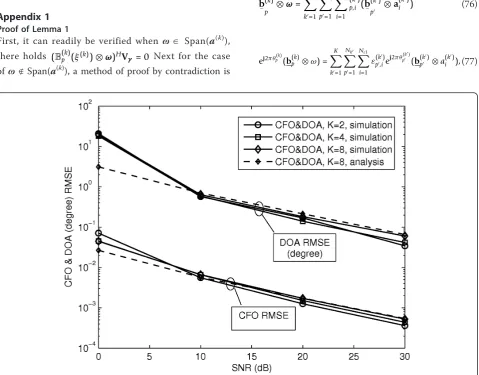
First, we consider the single cluster scenario, i.e.,Ncl= 1.
Both the CFO and DOA estimation performance versus SNR are shown in Figure 1. In this example, we setM= 2,
K= 4,Ls= 64 andL= 50, and the DOAs from set {30°,
45°, 95°, 100°}. Both the simulation and analytical results of the proposed method are presented in the figure. It is demonstrated that the analytical results closely match the simulations, especially under moderate or high SNR region, which verifies the correctness of our analysis. Besides, the performance of [18,19] are also presented for comparison, which are referred to as‘ESPRIT-1’and
‘ESPRIT-2’, respectively. Note that there is a similar smoothing parameterLin ESPRIT-1, which will be set the same as ours in the following unless otherwise stated. The results clearly demonstrate that substantial improvement can be achieved by our proposed method compared to the other two counterparts, especially in the lower SNR region. This can be explained as follows. First, we have exploited the smoothing technique in our method, which improves the estimation of the correlation matrix; Second
and more importantly, both ESPRIT-1 and ESPRIT-2 derive the CFO or DOA for each user by an indirect approach: they first estimate multiple CFO or DOA values separately for each occupied subcarrier of each user, and then combine them as the final result. Hence, lots of redundant parameters need to be estimated from the sub-space algorithm, making both ESPRIT-1 and ESPRIT-2 less efficient. However, in our method, we make use of the fact that there is only one CFO and only one DOA for each user, and these two parameters are directly estimated by the designed rank reduction approach.
Next, we evaluate the performance of our method in the multi-cluster scenarios withK= 4 users. Both two clusters, i.e.,Ncl= 2, and three clusters, i.e.,Ncl= 3, are
considered in this example. For Ncl = 2, the DOAs of
the users are set as {{30°, 50°},{60°, 70°}, {90°, 140°}, {120°, 160°}}, while for Ncl = 3, the DOAs are set as
{{30°, 50°, 140°}, {20°, 60°, 100°}, {90°, 110°, 140°}, {80°, 120°, 150°}. In addition, M= 4 and M = 6 are assumed forNcl = 2 andNcl = 3, respectively. Other parameters
are set asLs= 64 and L= 50. We depict the CFO and
DOA estimation performance of our method in Figure 2, where both simulation and analytical curves are included. As expected, the results demonstrate the
Figure 1The performance comparison of both CFO and DOA estimation RMSE versus SNR underNcl= 1 andM= 2. The top four
effectiveness of our method for multi-cluster scenarios. The analytical results also closely match the simulations. Combing the observations from Figures 1 and 2, we can conclude that, as compared to ESPRIT-1 [19] and ESPRIT-2 [18], our method not only has the advantage of being applicable to multi-cluster channels, but also can obtain much better performance in single cluster channels.
In this example, we assume SNR = 20 dB,M= 2, K= 4, andLs= 64, while the DOAs of the users are set the
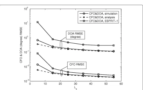
same as that in Figure 1. The estimation performance evolution of our method under the single cluster sce-nario is shown in Figure 3, with Lincreasing from the lower bound 49 calculated from (25)bto N= 64. The analytical results are presented by the dashed curves. For comparison, we also include the corresponding per-formance of ESPRIT-1 and ESPRIT-2. Note that since ESPRIT-2 does not have the parameter L, its perfor-mance is presented as a straight line parallel to the
x-axis. From the results, we observe an optional range of L that can be selected without considerable loss of performance, e.g., from 49 to 62 in this example. More-over, we see that, our method always obtains better DOA estimation performance than the other two candi-dates under all values of L. On the side of CFO
estimation, our method always behaves better than ESPRIT-1, while as compared to ESPRIT-2, our method behaves worse only whenL= 64. In addition, some mis-match appears between the simulation and analytical results of our method at the right-hand end of the curves. This is because that, whenL is very large, the estimation for the correlation matrixRg becomes worse, whose fluctuation may result in the occurrence of some outliers in simulations.
Afterwards, we investigate the performance of our method with the increasing ofLsin Figure 4, where the
DOA configuration is the same as that in Figure 3. Besides, we assume SNR = 20 dB,M= 2,K= 4, andL= 50 in this example. As expected, performance improve-ment can be observed with the increase of blocks adopted. Our method almost converges within 30 blocks. Moreover, it is seen that, in terms of both CFO and DOA estimation, our method behaves better than ESPRIT-1 under all values ofLs. Note that since ESPRIT-2 does not
work whenLs< 64, its performance is not included in
this figure. In addition, some mismatch appears between the analytical and simulation results of our method at the left-hand end of the curves. This is also because of the occurrence of outliers when a small number of blocks are adopted.
Figure 3The CFO and DOA estimation RMSE performance versusLunder the single cluster scenario. The top four curves correspond to the DOA RMSE (degree), while the bottom four curves correspond to the CFO RMSE.○: simulation results of the proposed method; dashed: analytical results of the proposed method;□: the method from [19];◊: the method from [18].