Volume 2008, Article ID 394201,11pages doi:10.1155/2008/394201
Research Article
Implementation of the Least-Squares Lattice with Order and
Forgetting Factor Estimation for FPGA
Zdenek Pohl, Milan Tichy, and Jiri Kadlec
Institute of Information Theory and Automation, Pod Vodarenskou vezi 4, 182 08 Prague, Czech Republic
Correspondence should be addressed to Milan Tichy,[email protected]
Received 6 February 2008; Revised 5 June 2008; Accepted 24 June 2008
Recommended by Ricardo Merched
A high performance RLS lattice filter with the estimation of an unknown order and forgetting factor of identified system was developed and implemented as a PCORE coprocessor for Xilinx EDK. The coprocessor implemented in FPGA hardware can fully exploit parallelisms in the algorithm and remove load from a microprocessor. The EDK integration allows effective programming and debugging of hardware accelerated DSP applications. The RLS lattice core extended by the order and forgetting factor estimation was implemented using the logarithmic numbers system (LNS) arithmetic. An optimal mapping of the RLS lattice onto the LNS arithmetic units found by the cyclic scheduling was used. The schedule allows us to run four independent filters in parallel on one arithmetic macro set. The coprocessor containing the RLS lattice core is highly configurable. It allows to exploit the modular structure of the RLS lattice filter and construct the pipelined serial connection of filters for even higher performance. It also allows to run independent parallel filters on the same input with different forgetting factors in order to estimate which order and exponential forgetting factor better describe the observed data. The FPGA coprocessor implementation presented in the paper is able to evaluate the RLS lattice filter of order 504 at 12 kHz input data sampling rate. For the filter of order up to 20, the probability of order and forgetting factor hypotheses can be continually estimated. It has been demonstrated that the implemented coprocessor accelerates the Microblaze solution up to 20 times. It has also been shown that the coprocessor performs up to 2.5 times faster than highly optimized solution using 50 MIPS SHARC DSP processor, while the Microblaze is capable of performing another tasks concurrently.
Copyright © 2008 Zdenek Pohl et al. This is an open access article distributed under the Creative Commons Attribution License, which permits unrestricted use, distribution, and reproduction in any medium, provided the original work is properly cited.
1. INTRODUCTION
A number of possible applicationsindigital signal processing
(DSP) such as parameter estimation [1], echo suppression
[2], or beam-forming [3] can be found for adaptive least
squares filters. Their recursive form known as therecursive
least squares (RLS)[4] is the solution of the minimum mean square error problem. The convergence rate of the RLS is far
superior to that of the well-knownleast mean square (LMS)
[5] algorithm and its normalized sibling NLMS.
The hardware implementation of the RLS algorithm is
rather difficult due to its high computational complexity
and problems with numerical stability. The complexity can be decreased by the exploitation of serial structure of the input data, typical for DSP applications. It allows to reduce
asymptotic complexity of the RLS fromO(N2) toO(N). One
of thefastversions of RLS algorithm is represented by thefast
transversal filters (FTF)[6–8]. The problems with numerical instability of the FTF lead to the development of its stabilized
version [9, 10]. Motivated to develop numerically stable
fast RLS filters, theleast-squares lattice (LSL)filters [11,12] andfast QR decomposition (QR-RLS)[13] algorithms were
developed. While the numerical stability of the fast
QR-RLS algorithm was proven analytically [14], good numerical
properties of an LSL filter were found experimentally. The
analysis of QR-RLS and LSL algorithms can be found in [15].
This work focuses on the LSL algorithm because of its slightly lower complexity.
The implementation of the LSL filter with error-feedback [16–18] has proven good numerical behavior. In [16], it was
shown that the filter can be efficiently implemented infield
programmable gate arrays (FPGA). In the following text, this
algorithm is referred to as theRLS lattice. Its computational
complexity is 24N, which can be further reduced by the
utilization of parallel hardware in an FPGA.
The possibilities of efficient FPGA implementation of
the RLS lattice algorithm were exhaustively investigated in
algorithms for FPGAs can be found in [21–23]. As shown in
these works, the resultingintellectual property (IP)cores can
outperform floating-point DSP microprocessor solutions by one order of magnitude. There also exist other RLS filter
FPGA implementations such as [1, 3], where IP cores are
implemented and integrated in a custom one purpose design.
Another implementation of RLS filter is presented in [24],
where calculations are distributed between FPGA and the NIOS microprocessor in a single chip.
Our aim is to provide a versatile highly configurable hardware RLS core for DSP applications. We focus on the implementation of a hardware coprocessor rather than a standalone IP core. Our target application scheme is to use one lattice filter and to estimate the order probability or
to use more parallel lattice filters with different forgetting
factors on a single channel and to estimate, which forgetting factor yields better results. We also expect that parallel lattice filters will be possible to interconnect serially and to create a high performance pipelined solution. The algorithm is integrated into the Xilinx EDK environment as a Microblaze accelerator, resulting in a versatile, easy-to-use and compact RLS lattice coprocessor, which can easily be accessed by the standard C programming and debugging.
2. PROBABILISTIC APPROACH TO SYSTEM
IDENTIFICATION
In order to outline the development of the RLS lattice algorithm with order probability estimation and to describe its hardware implementation, a brief insight to the recursive least squares estimation from the probabilistic theory view-point is provided.
The probabilistic approach [25] to the system
identi-fication provides the link between the probabilistic theory and the least square error estimation, which allows us to extend the estimation task by the hypotheses probability estimation. In this approach to the system identification, the hypotheses probability update of an autonomous
one-dimensional system [26] can be formulated as
p(hn|Dn)= p
(yn|Dn−1,hn)p(hn|Dn−1)
∀hp(yn|Dn−1,hn)p(hn|Dn−1)
, (1)
where ynare data observed at the unknown system output
at time n, the variables Dn and Dn−1 are previously
observed data y0 through yn and yn−1, respectively. The
hypothesis hn is the ordered pair h ∈ (i,λ), where i ∈
{0,. . .,N} is the unknown order and λ ∈ {λ1,. . .,λM} is
the unknown forgetting factor. The term p(yn|Dn−1,hn) is
the probabilistic description of the modeled system with
order and exponential forgetting given by hypothesishn. This
probability can be evaluated as
p(yn|Dn−1,hn)
=π−1/2λΛ
((λϑn−1−i)/2+1)
h,n−1
Λ((ϑn−i)/2+1) h,n
·det (λVz,h,n−1)
1/2
det (Vz,h,n)1/2 ·
Γ((ϑn−i)/2+1)
Γ((λϑn−1−i)/2+1),
(2)
whereΛhis the optimal solution error of the model for the
hypothesish. The matrixVz,h,nis the autocorrelation matrix
defined as
Vz,h,n=zh,nzTh,n, (3)
where
zh,n=[yn−1· · ·yn−i]T. (4)
The operatorΓin (2) is the gamma function. The quantityϑ
represents the “amount of data” accumulated in matrixVz,h,n
through the estimation process. The quantityϑis updated as
ϑn=λϑn−1+ 1. (5)
It should be noted that according to [25] the relation (2) is correct only for the definition of the autoregression model
inherent to the hypothesis h as a conditional probability
density function (pdf)
p(yn|Dn−1,Θh,n,hn)= √ωh,n
2πe
−(ωh,n/2)(yn−ATh,nzh,n)2, (6)
where the symbolΘh,ndenotes parametrization of the model
by the vector of unknown parametersαand of an unknown
precision measureω[25]
Θh,n= {Ah,n,ωh,n},
ATh,n=[α1 · · · αi].
(7)
The autoregression model of an unknown system in (6) can
be described as
yn=ATh,nzh,n+eh,n, (8)
whereeh,n is the prediction error of the model inherent to
the hypothesis h at time n. As shown in [25], if eh,n is a
normally distributed random variable, the conditional pdf
for the model parametersΘh,ncan be written as
p(Θh,n|Dn,hn)=ch,nωh,nϑn/2e−(ωh,n/2)Xh,n, (9)
wherech,nis a normalizing constant and
Xh,n=
−1
Ah,n T
Vh,n
−1
Ah,n.
. (10)
The matrix Vh,n is the augmented autocorrelation matrix
which keeps information about the shape of the conditional
pdf (9). This data matrix can be updated recursively as
Vh,n=λVh,n−1+λ
yn
zh,n yn z T h,n
. (11)
The optimal solutionAh,nforAh,nis located at the maximum
of the conditional pdf (9). The maximum can be found by
the minimization of the quadratic form (10), which can be
written as
Xh,n=Λh,n+ (Ah,n−Ah,n) T
For better clarity, the subscriptnwill be omitted in the
fol-lowing text. The matrixVhused in (10) can be decomposed
as follows:
Vh=
Vy VTz,y,h Vz,y,h Vz,h
. (13)
Consequently, the optimal solution can be written as
Ah=V−1z,hVz,y,h, ωh=ϑΛ−1h ,
(14)
where
Λh=Vy−VTz,y,hV−1z,hVz,y,h. (15)
Recursive formulas for the direct update of the decomposed
matrixVhcan be derived from (11).
The recursive solution forAh, maximizing the pdf given
by (9), is also known as the RLS algorithm [27]. It is
important to note that for the estimation of (N + 1)M
hypotheses by the Bayes formula (1), it is needed to estimate
all models defined by the estimated hypotheses, which means
to calculateNM-array of RLS filters.
3. HYPOTHESES ESTIMATION
Despite the possibility to implement the RLS estimation by
formulas introduced in Section 2, it is more convenient to
use one of the state-of-the-art RLS algorithms. As the most convenient algorithm for implementation, the recursive
least-squares lattice [4] in the error-feedback form was
chosen. As suggested in [17], the normalized a posteriori
errors are used to reduce the complexity of the algorithm.
The computational complexity of this algorithm is 24N,
whereNdenotes the filter order (dimension).
As mentioned above, the estimation of probability of
hypotheseshby (1) requires performing one RLS estimation
for each hypothesish. Thus, theNM-array of RLS filters has
to be calculated.
The most important property making the RLS lattice suitable for the hypotheses estimation is its modular struc-ture. The RLS lattice filter consists of a cascade of identical
modules. Each module implements theorder update, which
means that it is usingith order output from the preceding
module and increases the order of estimation to i + 1.
Consequently, estimations of all orders up toNcan be found
during computations. Using this principle, the number RLS filters required for the hypotheses estimation can be reduced toM.
In our solution, the evaluation of probability estimates is divided into two stages. The first stage performs the order update, which uses the “old” probability estimates and updates them by new data. This operation is represented by
the numerator of (1). In the second stage, thenormalization
of the updated order estimates is performed. The
normaliza-tion is represented by the denominator of (1). The forgetting
on hypotheses pdf is applied in the normalization stage. The order update can be integrated into the RLS lattice algorithm.
Initialization
γ−1=1,F−1=B−1=δI ψ−1=γ
f
−1=γb−1=κ−1=ba−1=0
e1, e2, g set using (17) and (18) Lattice update (for eachn≥0):
α0,n =dn,η0,n=ψ0,n=un,γ0,n=1 psd
−1,λ,n =(N+ 1)ϕ
for(i=0;i≤N;i=i+ 1) ηi+1,n =ηi,n−γ
f
i+1,n−1ψi,n−1 T1,2 f =γi,n−1ηi,n T3 ψi+1,n =ψi,n−1−γbi+1,n−1ηi,n T5,4
b =γi,nψi,n T6 αi+1,n =αi,n−κi+1,n−1ψi,n T8,7 γif+1,n =γ
f
i+1,n−1+bai,n−1ηi+1,n T10,9 Fi,n =ν+λFi,n−1+f ηi,n T13,11,14,12 Bi,n =ν+λBi,n−1+bψi,n T17,15,18,16
fa
i =f /Fi,n T19 ba
i,n =b/Bi,n T20 γb
i+1,n =γbi+1,n−1+ fiaψi+1,n T22,21 κi+1,n =κi+1,n−1+bai,nαi+1,n T24,23 γi+1,n =γi,n−bai,nb T26,25
a1 =λFi,n−1 U1 a2 =ae11i/Fie2,ni U2 a3 = |γi,n|1/2 U3 pd
i,λ,n =pi,λ,n−1·a2·a3·gi U4,5,6 psd
i,λ,n =pisd−1,λ,n+pdi,λ,n U7
end
Algorithm 1: RLS lattice algorithm with exponential forgetting and probability update evaluation. The labelsTxxandUxdenote individual arithmetic operations contained in the right side of each equation.
ηi,n ηi+1,n
ψi,n ψi+1,n
αi,n αi+1,n
Bi,n−1
Fi,n−1
κi,n−1
z−1
Figure 1: Data flow graph of one order update step of the algorithm.
The RLS lattice algorithm with order and forgetting factor
update is summarized inAlgorithm 1. For the illustration,
the update of estimates to orderi+ 1 from orderiis depicted
inFigure 1.
The algorithm presented inAlgorithm 1is in the form,
where input un is used to estimate desired value dn. For
identification of one-dimensional autoregression model the
yn un αN,n z−1
dn
pn−1 pn
z−1 RLS lattice
Order estimation
Figure 2: RLS lattice algorithm for identification of one-dimensional autoregression model.
Table 1: The parameters of the RLS lattice algorithm with exponential forgetting and probability update evaluation.
Parameters
N Filter order
λ∈(0; 1 Forgetting factor
δ δ >0,δ→0 Regularization parameter ν 2−b(1−λ) Regularization constant ϕ∈ 0; 1) Hypotheses forgetting factor
probabilistic approach given in Section 2 can be used for
estimation of order and forgetting factor probability as also shown in the figure. The RLS lattice algorithm parameters
are summarized inTable 1.
For the probabilityp(hn|Dn),ph,n=pi,λ,nwill be further
used as a more simple notation, wherehwas defined as the
ordered pair (i,λ),i ∈ {0,. . .,N},h ∈ {1,. . .,M}. Before the first iteration of the algorithm, initial hypotheses pdf has to be set and the look-up tables have to be initialized. The initial hypotheses pdf can be selected as
pi,λ,−1= 1
(N+ 1)M ∀i,λ, (16)
wherepi,λ,nis the probability of orderiand forgetting factor
λat timen. Valuen = −1 represents the initialization step.
The look-up tables are initialized for the limit value of
ϑlim=lim n→∞ϑn=
1
1−λ (17)
as follows:
e1i= λϑlim−i
2 + 1
e2i= ϑlim−i
2 + 1 i=0,. . .,N
gi=π−1/2Γ(e2i)
Γ(e1i)
. (18)
After the values pi,λ,n−1 have been updated, the
nor-malization step has to be performed to obtain actualized
probability pi,λ,n. The pdf given by (1) extended with
forgetting of hypotheses can be evaluated as
pi,λ=
pdi,λ+ϕ λM
λ=λ1
N
i=0(pdi,λ+ϕ)
, (19)
where pdi,λ is updated, but not normalized probability of
orderiand forgetting factorλ. The symbolϕis the forgetting
factor of hypotheses.
Equation (19) can be calculated more efficiently as
pi,λ= pd
i,λ+ϕ λM
λ=λ1p
sd N,λ
, (20)
wherepNsd,λis a sum of updated probabilitiespdi,λbiased by the
forgetting factor of hypotheses. Comparing (19) and (20), it
can be shown that the sum of updated probabilities pdi,λcan
be calculated as
psd N,λ=
N
i=0
(pd
i,λ+ϕ)=(N+ 1)ϕ+ N
i=0 pd
i,λ. (21)
Then, the value of psdi,λis calculated using the update of psdi,λ
from its initial valuepsd−1,λ=(N+ 1)ϕas shown in the
right-hand side of (21). This step is labeled as operation U7in
Algorithm 1.
Adding the order and forgetting estimation, the original
RLS lattice algorithm increases its complexity to 31N. Thus,
the number of operations for maintainingN+1 order andM
forgetting factor hypotheses is 31NM. The normalization of
updated probabilities requires 2M(N+1)+M−1 operations.
Considering these figures, we can state the complexity of the RLS lattice with the estimation of hypotheses which is
33NM+ 3M−1 operations, provided that the division of
two powers is regarded as one operation.
It is evident that the implementation ofM RLS lattice
estimations to test each hypothesis can be easily parallelized. For each forgetting factor hypothesis, one RLS lattice instance extended by the probability update can be evaluated in parallel. When all filters have been calculated, the normal-ization is performed before new data are acquired. Such an
arrangement can be efficiently implemented in FPGAs.
4. FPGA IMPLEMENTATION
Hardware implementation of the RLS lattice requires ALU providing ADD, SUB, MUL, and DIV operations. For the probability estimation, POW and SQRT operations are also
required. TheLogarithmic Number System (LNS)arithmetic
[28, 29] has been identified as the most convenient
alter-native to floating point for hardware implementation. This selection is supported by [16,19].
Numbers in LNS are represented as fixed-point base-2 logarithms of numbers to be represented. The LNS
arithmetic provides extremely effective MUL, DIV, and
SQRT operations. The ADD/SUB operations are more complex and thus require more resources. For our RLS
lattice implementation, thehigh speed logarithmic arithmetic
(HSLA)library was used [29].
The proposed hardware provides solution to a few implementation challenges, such as
(i) conversions between fixed-point and LNS numbers; (ii) implementation of the power function or directly of
(iii) mapping the algorithm to the LNS ALU efficiently and scheduling of operations;
(iv) ensuring the numerically robust behavior; (v) implementation of the optimized RLS lattice core; (vi) supporting integration of the core into a
Micropro-cessor system.
In the following sections, these issues are directly addressed and their solution is presented.
4.1. Conversions
In audio DSP applications, the 16-bit two’s complement integer is a typical input and output data format. The same precision was used for implementation of the input and output of the RLS lattice filter.
A conversion of an unsigned 16-bit fixed-point numbers
to LNS format and vice versa, introduced in [19], was
implemented. The method can be easily modified for signed integers. The integer to LNS conversion is based on the LNS addition, which can be written as
log2(X+Y)=i+ log2(1 + 2j−i), (22)
where i = log2|X| and j = log2|Y| are the fixed-point
numbers representingXandYin LNS, respectively. The
16-bit integer input can be written as
Z=28z
1+z2, (23)
where z1 and z2 are high and low parts of the integer Z,
respectively. Then, the conversion ofZinto the LNS can be
written as
log2Z=log2(28z1+z2)=log2(X+Y). (24)
It is clear that for calculation of the LNS image of Z, the
valuesi = log2|X| = log2|28z1|and j = log2|z2| have to
be known. The value ofiandjcan be tabulated asTiandTj,
each of depth 256.
The conversion from LNS to fixed point is implemented
as the binary search of the nearest lower number inTi. The
value ofTi is then subtracted from the original in the LNS
domain and the search continues inTj. The integer result
is formed from addresses of found values in the tablesTiand
Tj. The hardware solution of conversions using LNS addition
and two tables delivers maximal conversion performance for the input and output data.
Initialization of the algorithm presented inAlgorithm 1
requires constants and initial vector values in LNS. A software conversions for an FPGA soft processor were implemented using the functions provided in HSLA.
4.2. Division of powers
As mentioned inSection 2, the division of two general
pow-ers in (2) is considered as one floating-point-like operation.
In the LNS arithmetic, this operation can be calculated as
Z=log2A e1i
Be2i =a·e1i−b·e2i, (25)
wherea=log2|A|andb=log2|B|are LNS representations
ofAandB, respectively. The values ofe1ande2are
fixed-point exponent values stored in tables defined in (18).
According to (25), the division of two powers in the
LNS can be implemented very efficiently as the
fixed-point multiplications, which are in fact fixed-fixed-point integers representing base-2 logarithm with a fixed-point expo-nent. Consequently, the results are subtracted. The FPGA implementation benefits from the possibility to use integer subtraction in full precision and to truncate the result to the desired LNS width at the end.
The fixed-point exponents in tablese1ande2are stored
in 16-bit unsigned fixed-point with 8 fractional bits. Such
decision makes possible efficient implementation without
the loss of precision. Although such representation limits the
possible range of the parameterλtoλ ∈ 0.95; 0.995and
of the parameteritoi∈ {0; 20}, this range covers the most
used options for the recursive identification and for the order
estimation. The restriction put on the order icorresponds
with the range in which the probabilistic approach to order
estimation can provide reliable results as shown in [30].
4.3. ALU and scheduling
Since our implementation of the RLS lattice filter is designed for 16-bit two’s complement integers used as an input
and output, the 19-bit LNS arithmetic provides sufficient
precision. The bit allocation within the 19-bit LNS number is as follows: 1 bit sign and 18-bit two’s complement fixed-point number. Special values are reserved for zero, NaN, and Inf.
In order to exploit the maximal possible parallelism in the implementation of the RLS lattice filter, the cyclic
scheduling of the RLS lattice inner loop was used [20,31].
It was found that the addition hardware macro is utilized by less than 25%. For higher utilization of resources, four RLS lattice filter modules can share one dual-port ADD/SUB unit, that is, four independent RLS lattice filters can be implemented without using more ADD/SUB units. Other hardware macros used in the RLS lattice filter implemen-tation are four MUL and DIV macros, one SQRT, and POW/POW macro. All hardware macros are fully pipelined.
Using the method of cyclic scheduling, four independent RLS lattice filter modules were mapped onto the LNS arithmetic units so that the schedule consists of 2 clock cycles prologue loop, 25 clock cycles main body loop, and 34 clock cycles epilogue loop. The resulting schedule is depicted
in Figure 3, where the evaluation of one iteration of the
RLS lattice filter is displayed. Operations for one iteration
of the algorithm presented in Algorithm 1are spread over
three consecutive iterations in the hardware implementation
and evaluated concurrently. Operations inAlgorithm 1were
labeled T1-26 for the RLS lattice algorithm and U1-7 for
the probability update. InFigure 3, the corresponding
oper-ations are displayed as 4-clock-cycle long operoper-ations, which consist of four consecutive calls—one for each instance of the RLS lattice module.
4.4. Numerical behavior
To guarantee the numerical stability, it is required to avoid
U9 U8 U3
U2
T19
T20 U10
T11 cont. T4 T6 U11 T11
T21
cont. T23 T7 T12 T21
T15 T1 T3 T9 T25
U4 cont. U5 T16 U1 U6 U4
T26 cont. T17 T2 T18 U7 T22 T26
T13 T5 T8 T14 T10 T24
Txx Txx
Uxx
Txx
Uxx LSL
algorithm
Extension
Operations in iterationi−1
Operations in iterationi Operations in iterationi
Operations in iterationi+ 1
Operations in iterationi+ 1 Clock cycles
1 2 3 4 5 6 7 8 9 10 11 12 13 14 15 16 17 18 19 20 21 22 23 24 25 ADD/SUB1
ADD/SUB2 MUL0 MUL1 MUL2 MUL3 DIV0 DIV1 POWSD SQRT Macro
instances w
Figure3: Schedule of operations of four RLS lattice algorithms with probability estimation. The operationsTxxandUxare defined in Algorithm 1.
T6 T16
T15 T20
ν0 (a) Nonbiased
T6
T16
T15 T20
ν
(b) Biased
Figure 4: Comparison of two approaches to regularization of division inT20. The critical path fragment is marked in red.
The sufficient solution is to add a small positive constantν0
to the denominator before the divisions are evaluated [18].
Such solution providesnonbiasedenergiesBi,nandFi,n.
Alternatively, the constantν=ν0(1−λ) can be used in
operations labeledT13andT17[17]. We use this version of
the RLS lattice which introduces a small bias to the energies
Bi,nandFi,n.
The “biased” version is more suitable for parallelization, rather than using the nonbiased version, because the
eval-uation of the energy Bi,n lies on the critical path of the
algorithm. Situation on the critical path is compared to both
options inFigure 4. It can be seen that at the expense of a
small bias added to the energiesFi,n andBi,n, the iteration
time of the lattice loop is decreased from 33 to 25 clock cycles, that is, by 24%.
According to [17,18], the constantνequal to 2−b(1−λ)
should be used. Here, b is the mantissa length to which
the prediction energies are quantized andλis the forgetting
factor. For the 19-bit LNS arithmetic case,b =12 was used.
The worst case forgetting factor λ = 0.95 is determined
by constrain introduced inSection 4.2. The relation forνis
correct under the assumption that input signal ynis within
the range −1, 1, which is always satisfied by the input and
output conversions described inSection 4.1.
4.5. Optimized RLS lattice core
The result of RLS lattice implementation is a standalone IP core. The internal variables of the core are expected to be stored in external memories. It allows more convenient integration of the core into the soft core processor.
A special memory organization, grouping the instances of one internal variable into one distributed memory ele-ment, was used. It allows us to reduce the size of multiplexer connected to the shared arithmetic unit macros, which is
demonstrated inFigure 5. The experiments show that 8% of
FPGA resources was saved by this approach.
4.6. Integration to a microprocessor system
against one purpose design based on the same core. The
XSG schematic of the coprocessor can be seen inFigure 6.
It consists of the RLS lattice core denoted LSL, which can
also be used as a standalone core of the input and output
data buffers denotedinBuf andoutBuf, of the control words
mb2hc controlandhc2mb status, and of the communication
interface denotedComm.
TheCommblock is responsible for the batch processing
of input data by the RLS lattice core in theLSLblock. It stores filter results to the output buffer. It is capable of working with the RLS lattice core containing one up to four filter instances.
The LSL module consists of order updating loop (see
algorithm inAlgorithm 1) with the input consisting of four
values. After increasing the estimation to higher order, the same four data can be regarded as output. Otherwise, only the internal states are altered. As a consequence, one filter can use another filter output as its input and to continue in the computation of order updates. The solution of higher-order filter can be obtained using the pipelined solution consisting of multiple RLS lattice filter instances. That is why
theCommblock in the coprocessor design has to be capable
of reconfiguring data path between RLS lattice instances, in order to use them either as parallel four channel RLS lattice filter (each with order up to 126), or it is possible to connect up to four instances serially and to create pipelined
RLS lattice solution with order up to 504, achieving 4×
higher performance. It is the reason why, inFigure 6, thefifo
block storing the intermediate results is used in the pipelined organization of the coprocessor.
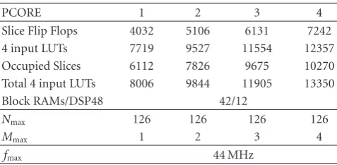
Four versions of the PCORE with one, two, three, and four RLS lattice modules were implemented. Resource requirements in the Xilinx Virtex4 SX35 device are
sum-marized in Table 2. For illustration, the floor-plan of the
system with Microblaze and the PCORE with four RLS lattice
modules as a coprocessor are presented inFigure 7. The area
occupied by the Microblaze processor is displayed in yellow, the FSL communication interfaces in blue, batch processing control unit in purple, and the RLS lattice filter core in green color. The entire system occupies 78% of the Xilinx Virtex4 SX35 chip.
5. DYNAMIC RECONFIGURATION
The implementation of the RLS lattice as a coprocessor con-nected to the Microblaze makes possible to use the dynamic reconfiguration for loading and unloading the coprocessor while the microcontroller is running. The loading of the coprocessor can be initiated on demand.
The software version of the RLS lattice filter was devel-oped. The floating-point number representation is used in the Microblaze, whereas the 19-bit LNS is used in hardware. The software conversions based on the HSLA library were used for implementation of migration between hardware and software. The conversions are based on evaluation of base-2 logarithm contained in the Microblaze glibc library. Such conversions are time consuming even if a hardware support of floating-point is included in the Microblaze.
To control the load of the processor and the power consumption, a mechanism for migration the task from
Address
Lattice 1 data A Lattice 1
data A
data A data A Lattice 2 Lattice 2
mux
MUL
Lattice 1–4 data B Grouping memories together
Lattice 1 Lattice 2 Lattice 3 Lattice 4 Lattice 1–4 address
Mem A mux
MUL
Lattice 1–4 data B
Figure5: Reduction of multiplexers by grouping the block mem-ories.
Table 2: RLS lattice coprocessor resources usage in the Xilinx Virtex4 SX35 device.
PCORE 1 2 3 4
Slice Flip Flops 4032 5106 6131 7242
4 input LUTs 7719 9527 11554 12357
Occupied Slices 6112 7826 9675 10270 Total 4 input LUTs 8006 9844 11905 13350
Block RAMs/DSP48 42/12
Nmax 126 126 126 126
Mmax 1 2 3 4
fmax 44 MHz
the processor to coprocessor was developed. The software version of the RLS lattice runs in the Microblaze when no other tasks require to use the processor. When there is a need to use the Microblaze for other tasks, the processor is freed and the RLS lattice is run in the coprocessor.
The available run-time configurations are presented in
Figure 8. One is the software solution, remaining three are the coprocessor versions containing one to four RLS lattice filters.
6. PERFORMANCE RESULTS
The performance in each run-time state was measured
and the key results are summarized in Table 3. The table
is divided into three parts. The first part summarizes performance of the RLS lattice filter with the probability estimation. In general, the estimation of the model order higher than 15–20 is not giving satisfactory results, as it
was shown in [30]. Thus, higher order of estimation is not
expected to be used. As it can be seen in the table, the performance decreases with the number of employed RLS lattice instances. The performance of hardware coprocessor
is 5.5-times higher compared to the software solution, even if
the clock frequency of the microprocessor is 4-times higher (this can be seen in the table by comparison of Microblaze
System generator
EDK processor MB
dout
mb2hc control
[a:b]
Slice bit[0]
DelayZ
Delay RDY
Shared memory
<<‘fifo’>>
Comm CommSim
Shared memory
<<‘outBuf ’>> z−1
z−1
Shared memory
<<‘inBuf ’>>
LSL hc2mb status
fifoMemDOUT
inBufDOUT
lattice rdy
lattice z
mb2hc
outBufDOUT
rst
fifoMemADDR
fifoMemDIN
fifoMemWEN
hc2mb
inBufADDR
inBufDIN
inBufWEN
lattice a
lattice en
outBufADDR
outBufDIN
outBufWEN
addr
din we
dout
addr
din
we dout
a
en
rst
rdy z stages order contexts
din stages order contexts
addr
din
we dout
Figure6: The RLS lattice coprocessor integration to Microblaze processor via FSL.
Table3: Performance of the RLS lattice coprocessor: the execution time for 180 inputs is presented.
Processor Clk [MHz] M N Time (ms) Mflops
Microblaze 100 4 16 69.46 5.50
PCORE1 25 1 16 12.24 7.79
PCORE2 25 2 16 12.96 14.74
PCORE4 25 4 16 12.49 30.60
Microblaze 100 4 126 547.53 3.98
PCORE1 25 1 126 29.60 18.39
PCORE2 25 2 126 29.40 37.02
PCORE4 25 4 126 28.70 75.86
PCORE4 pipe 25 1 64 7.02 39.38
PCORE4 pipe 25 1 504 26.48 82.22
Figure 7: Floor-plan of the RLS lattice filter implementa-tion: Microblaze processor (yellow), FSL communication interface (blue), batch processing control (in purple) and the RLS lattice core (green); the Xilinx Virtex4 SX35 usage is 78%.
The second part shows results with the probability estimation deactivated. The results for maximal supported
Microblaze
PCORE4 PCORE2
PCORE1
State reorganization State conversion
Figure8: Reconfiguration states with switch possibilities.
4000 3500 3000 2500 2000 1500 1000 500 0
n
−1 0 1 2
Or
der
Real order
(a)
4000 3500 3000 2500 2000 1500 1000 500 0
n 0
0.2 0.4 0.6 0.8 1
Order probability
Order 0 Order 1
(b)
Figure9: The order probability evaluation for orders 0 and 1.
cyclic scheduling. The acceleration of computation is nearly 20-times compared to the software solution running at 4-time higher clock speed.
The last part of the table shows results for the pipelined version of the RLS lattice filter. The pipelined solution uses
all four RLS lattice instances, each computing 1/4 of overall
estimation order. The hardware solution of order 504 is
equivalent to software with M = 4 and N = 126, and
the speedup of 20-times is reached again. The performance of the pipelined solution can be seen in the last row of
Table 3. In the pipelined solution, the probability estimates cannot be maintained because the normalization cannot be implemented in such case.
The switch cost between run-time states was measured.
The time for conversion is 411μs/order. To change the state,
local memories in the PCORE have to be reorganized. The time required for this state change was found by another
experiment as 4μs/order. Thus, we can formulate the “reorg”
state and conversion times, which areTreorg =4MN μs and
Tconv=411MN μs, respectively.
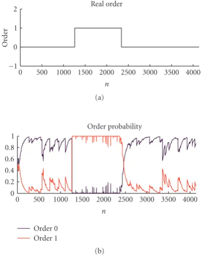
The example of order estimation is presented inFigure 9.
The upper plot shows the time when the model order was switched from 0 to 1 and back. The bottom plot shows the corresponding probability of order 0 and 1.
7. RELATED WORK
The error feedback RLS lattice filter algorithm was
imple-mented before, which is presented in [32]. Our
implementa-tion of the lattice PCORE has similar performance. However, three more lattice filters are possible to run at the same time and hypotheses probability can be evaluated in our
implementation. We have also demonstrated that four filters in coprocessor can be serialized to perform as one, 4-level pipelined filter. The performance can be 4-times better but the hypotheses estimation cannot be maintained.
There exists another RLS filter FPGA implementation
presented in [33]. The performance cannot be compared
since the only information provided in the paper is the clock frequency 5.3 MHz and the resource usage consisting of 2685 slices and 7 multipliers for the floating-point version and 3971 slices and 24 multipliers for the 17-bit LNS version (at 4 MHz). The PCORE implemented in our work uses 19-bit LNS and it can run at 44 MHz. In the smallest configuration, it occupies 4032 slices, 42 BRAMs, and 12 DSPs.
Our implementation is based on the algorithm presented
in [17]. Its implementation for the analog devices 21061
DSP (SHARC) running at 50 MHz allows to evaluate order
N = 290 at 8 kHz sampling rate. From Table 3 it can be
extrapolated that our solution at 44 MHz can, in the case
of one lattice module, operate for orderN =168 at 8 kHz
sampling rate (1.7×slower than SHARC solution). When all
four RLS lattice modules are used, the pipelined solution can
theoretically reach up toN = 753. However, the limitation
of the current implementation allows maximal value ofN=
504 (1.7× faster than SHARC). Alternatively, the filter of
orderN = 290 can operate at the sampling rate of 20 kHz
(2.5×faster than SHARC). It is important to note that our
architecture allows to execute any task on the microprocessor while the RLS lattice coprocessor is busy.
8. CONCLUSIONS
The easy use and easy programming and debugging PCORE integrated in the Xilinx EDK can perform 5-times faster than the software solution for Microblaze. At the maximal order with deactivated probability estimation, the acceleration reaches up to 20 times.
The dynamic reconfiguration can be used to adapt DSP capabilities to actual demand by changing the contents of the RLS lattice coprocessor. The migration of processing from
the microprocessor to HW requires 411NM microseconds,
whereNis the order andMis the number of filter instances.
The time is determined mainly by the conversion from the Microblaze floating-point representation to the LNS.
In the case of reconfiguration between different hardware
versions, the reorganization of the internal state takes only
4NM microseconds. The reconfiguration controller must
be designed with respect to the high cost of the migration between software and hardware solutions.
ACKNOWLEDGMENTS
REFERENCES
[1] Z. Salcic, J. Cao, and S. K. Nguang, “A floating-point FPGA-based self-tuning regulator,”IEEE Transactions on Industrial Electronics, vol. 53, no. 2, pp. 693–704, 2006.
[2] F. Capman, J. Boudy, and P. Lockwood, “Acoustic echo cancel-lation using a fast QR-RLS algorithm andmultirate schemes,” inProceedings of the 20th IEEE International Conference on Acoustics, Speech and Signal Processing (ICASSP ’95), vol. 2, pp. 969–972, Detroit, Mich, USA, May 1995.
[3] A. Nakajima, M. Kim, and H. Arai, “FPGA implementation of MMSE adaptive array antenna using RLS algorithm,” in Proceedings of the IEEE Antennas and Propagation Society International Symposium, vol. 3A, pp. 303–306, Washington, DC, USA, July 2005.
[4] S. Haykin,Adaptive Filter Theory, Prentice-Hall, Upper Saddle River, NJ, USA, 4th edition, 2002.
[5] B. Widrow and S. Stearns,Adaptive Signal Processing, Prentice-Hall, Englewood Cliffs, NJ, USA, 1985.
[6] G. Carayannis, D. Manolakis, and N. Kalouptsidis, “A fast sequential algorithm for least-squares filtering and predic-tion,” IEEE Transactions on Acoustics, Speech, and Signal Processing, vol. 31, no. 6, pp. 1394–1402, 1983.
[7] J. Cioffiand T. Kailath, “Fast, recursive-least-squares transver-sal filters for adaptive filtering,”IEEE Transactions on Acoustics, Speech, and Signal Processing, vol. 32, no. 2, pp. 304–337, 1984. [8] L. Ljung, M. Morf, and D. Falconer, “Fast calculation of gain matrices for recursive estimation schemes,”International Journal of Control, vol. 27, no. 1, pp. 1–19, 1978.
[9] J.-L. Botto and G. V. Moustakides, “Stabilizing the fast Kalman algorithms,”IEEE Transactions on Acoustics, Speech, and Signal Processing, vol. 37, no. 9, pp. 1342–1348, 1989.
[10] D. T. M. Slock and T. Kailath, “Numerically stable fast transversal filters for recursive least squares adaptive filtering,” IEEE Transactions on Signal Processing, vol. 39, no. 1, pp. 92– 114, 1991.
[11] D. Lee, M. Morf, and B. Friedlander, “Recursive least squares ladder estimation algorithms,”IEEE Transactions on Acoustics, Speech, and Signal Processing, vol. 29, no. 3, pp. 627–641, 1981. [12] F. Ling, D. Manolakis, and J. Proakis, “Numerically robust least-squares lattice-ladder algorithms with direct updating of the reflection coefficients,”IEEE Transactions on Acoustics, Speech, and Signal Processing, vol. 34, no. 4, pp. 837–845, 1986. [13] J. M. Cioffi, “The fast adaptive ROTOR’s RLS algorithm,”IEEE Transactions on Acoustics, Speech, and Signal Processing, vol. 38, no. 4, pp. 631–653, 1990.
[14] P. A. Regalia, “Numerical stability properties of a QR-based fast least squares algorithm,” IEEE Transactions on Signal Processing, vol. 41, no. 6, pp. 2096–2109, 1993.
[15] P. A. Regalia and M. G. Bellanger, “On the duality between fast QR methods and lattice methods in least squares adaptive filtering,”IEEE Transactions on Signal Processing, vol. 39, no. 4, pp. 879–891, 1991.
[16] F. Albu, J. Kadlec, C. Softley, et al., “Implementation of (normalised) RLS lattice on virtex,” in Proceedings of the 11th International Conference on Field Programmable Logic and Applications (FPL ’01), pp. 91–100, Springer, Northern Ireland, UK, August 2001.
[17] A. H. C. Carezia, P. M. S. Burt, M. Gerken, M. D. Miranda, and M. T. M. Da Silva, “A stable and efficient DSP implementation of a LSL algorithm for acoustic echo cancelling,” inProceedings
of the IEEE International Conference on Acoustics, Speech and Signal Processing (ICASSP ’01), vol. 2, pp. 921–924, Salt Lake City, Utah, USA, May 2001.
[18] M. D. Miranda, M. Gerken, and M. T. M. Da Suva, “Efficient implementation of error-feedback LSL algorithm,”Electronics Letters, vol. 35, no. 16, pp. 1308–1309, 1999.
[19] A. Herm´anek, Z. Pohl, and J. Kadlec, “FPGA implementation of the adaptive lattice filter,” in Proceedings of the 13th International Conference on Field Programmable Logic and Applications (FPL ’03), pp. 1095–1098, Springer, Lisbon, Portugal, September 2003.
[20] Z. Pohl, J. Kadlec, P. Sucha, and Z. Hanzdlek, “Performance tuning of iterative algorithms in signal processing,” in Pro-ceedings of the International Conference on Field Programmable Logic and Applications (FPL ’05), pp. 699–702, Tampere, Finland, August 2005.
[21] A. Heˇrm´anek, J. Schier, and P. A. Regalia, “Architecture design for FPGA implementation of finite interval CMA,” in Proceedings of the European Signal Processing Conference (EUSIPCO ’04), pp. 2039–2042, Vienna, Austria, September 2004.
[22] A. Heˇrm´anek, J. Schier, P. Sucha, and Z. Hanz´alek, “Opti-mization of finite interval CMA implementation for FPGA,” in Proceedings of the IEEE Workshop on Signal Processing Systems Design and Implementation (SIPS ’05), pp. 75–80, Athens, Greece, November 2005.
[23] P. Sucha, Z. Hanzalek, A. Heˇrm´anek, and J. Schier, “Scheduling of iterative algorithms with matrix operations for efficient FPGA design–implementation of finite interval constant mod-ulus algorithm,”The Journal of VLSI Signal Processing, vol. 46, no. 1, pp. 35–53, 2007.
[24] M. Karkooti, J. R. Cavallaro, and C. Dick, “FPGA imple-mentation of matrix inversion using QRD-RLS algorithm,” in Proceedings of the 39th Asilomar Conference on Signals, Systems and Computers, pp. 1625–1629, Pacific Grove, Calif, USA, October-November 2005.
[25] V. Peterka, “Bayesian approach to system identification,” in Trends and Progress in System Identification, P. Eykhoff, Ed., pp. 239–304, Pergamon Press, Oxford, UK, 1981.
[26] J. Kadlec,Probabilistic identification of regression model in fixed point, Ph.D. thesis, UTIA CAS, Bolivar, Tenn, USA, September 1986.
[27] J. Kadlec, “Lattice feedback regularised identification,” in Pro-ceedings of the 10th IFAC Symposium on System Identification (SYSID ’93), pp. 277–282, Copenhagen, Denmark, 1993. [28] J. N. Coleman, E. I. Chester, C. I. Softley, and J. Kadlec,
“Arithmetic on the European logarithmic microprocessor,” IEEE Transactions on Computers, vol. 49, no. 7, pp. 702–715, 2000.
[29] R. Matouˇsek, M. Tichy, Z. Pohl, J. Kadlec, C. Softley, and N. Coleman, “Logarithmic number system and floating-point arithmetics on FPGA,” inProceedings of the 12th International Conference on Field-Programmable Logic and Applications: Reconfigurable Computing Is Going Mainstream (FPL ’02), vol. 2438, pp. 627–636, Springer, Montpellier, France, September 2002.
[30] J. R. Dickie and A. K. Nandi, “A comparative study of AR order selection methods,”Signal Processing, vol. 40, no. 2-3, pp. 239– 255, 1994.
[32] F. Albu, J. Kadlec, N. Coleman, and A. Fagan, “Pipelined implementations of the a priori error-feedback LSL algorithm using logarithmic arithmetic,” inProceedings of the IEEE Inter-national Conference on Acoustics, Speech and Signal Processing (ICASSP ’02), vol. 3, pp. 2681–2684, Orlando, Fla, USA, May 2002.