A Twofold Sink Based Data Collection for Continuous Object Tracking in
Wireless Sensor Network
Chauhdary Sajjad Hussain *, Ali Hassan, Mohammed A. Alqarni, Abdullah Alamri Faculty of Computing and Information Technology,
University of Jeddah, Saudi Arabia. *Correspondence: [email protected]
SUMMARY
Continuous object tracking in WSNs, such as monitoring of mud-rock flows, forest fires etc., is a challenging task due to characteristic nature of continuous objects. They can appear randomly in the network field, move continuously, and can change in size and shape. Monitoring such objects in real-time generally require tremendous amount of messaging between sensor nodes to synergistically estimate object’s movement and track its location.
In this paper, we propose a novel twofold-sink mechanism, comprising of a mobile and a static sink node. Both sink nodes gather information about boundary sensor nodes, which is then used to uniformly distribute energy consumption across all network nodes, thus helping in saving residual energy of network nodes. Numerous object tracking schemes, using mobile sink, have been proposed in the literature. However, existing schemes employing mobile sink cannot be applied to track continuous objects, because of momentous variation of network topology. Therefore, we present in this paper a mechanism, transformed from K-means algorithm, to find the best sensing location of the mobile sink node. It helps to reduce transmission load on the intermediate network nodes situated between static sink node and the ordinary network sensing nodes. The simulation results show that the proposed scheme can distinctly improve life time of the network, compared to one-sink protocol employed in continuous object tracking.
Keywords: wireless sensor network; object tracking; dual sink; data collection
1.
Introduction
Various schemes have been employed to address the issue of tracking continuous objects such as gas spreads, mud or rock flows, spread of forest fires, volcanic eruptions, and so on. In such cases, a significant number of sensor nodes participate in boundary detection and at the same time continuously monitor whether critical data sensed by any node exceeds pre-defined threshold value. When sensed value measured by any sensor node exceeds a specified threshold value, it is considered to be in the region of interest. Among all the sensor nodes lying within such region of interest, only those nodes are selected which are situated at the peripheral boundary [1, 2]. Sensor nodes can locally determine whether they are boundary sensor nodes or not, by comparing their sensed values with their one-hop neighbouring nodes.
Generally, in WSN, all the data collected by sensor nodes is directed back to the sink node. Sensor nodes lying relatively closer to the sink node will inevitably participate more in data transmission, while forwarding data bound for sink node. These sensor nodes situated in the surroundings of the sink node are subject to rapid energy consumption due to additional traffic load. Sensor nodes generally are battery powered and have limited, non-renewable energy capacity [3]. Consequently, such nodes deplete their battery power completely and create holes in the network. To ensure uniform and fair energy utilization, the proposed scheme augments the network with a mobile sink node, capable of changing its physical location within the network topology.
It is worth mentioning that in this special case of continuous object tracking, the movement of this phenomena is dynamic; it changes its shape, size, and location. To collect information from a small localized section of the boundary sensor nodes, the data packets need to traverse large number of intermediate nodes before reaching static sink node. The moving ability of mobile sink node can resolve this problem effectively.
The mobile sink node employs k-means algorithm to calculate a physical location in the network, such that, the hop count distance between itself and the boundary nodes is minimum. Both static and mobile sink nodes collaborate with each other while calculating next optimized location for mobile sink node. Consequently, the transmission of data will require fewer intermediate hop traversals, reducing overall hop counts as well as transmission costs by conserving energy.
In this paper, we focus on how to find out optimized new location of mobile sink node by considering relative locations of the target boundary nodes and static sink node. We argue that in a cluster of wireless sensor nodes, when the cluster head is located at centric point of the cluster, each node will consume same amount of energy to transfer data to the cluster head . Therefore, we try to divide the boundary sensor nodes into two clusters, in each of which, there is a sink locates at the centric of cluster. Figure 1 illustrates the boundary sensor nodes selection and clustering. As shown in the figure 1(c), by computing the location of the boundary sensor nodes and static sink node, mobile sink would move to the centric point of cluster which it locates in. Likewise, it is more realistic to consider three-dimensional space, we examine only two-dimensional space in our architecture for simplicity. It is introduced in detail in section 4.
The rest of this paper is organized as follows: Section 2 discusses previous works and explores their shortcomings. In section 3, we present definitions as well as assumptions required for our algorithm. Section 4 presents the proposed algorithm in detail. Section 5 provides performance analysis of our algorithm with mathematics and simulation. Finally, in Section 6, we conclude our paper.
2.
Related Work
There has been abundant researches on detecting and tracking single or multiple targets in sensor network [1][3]. Recently, some researchers have begun to analyse detection and monitoring of continuous objects such as forest fires, mud flows, bio-chemical material diffusion and oil spills [2].
In DEMOCO [2] an energy efficient algorithm is proposed to detect and monitor continuous objects. A sensor node for which the present sensing is changed from the prior time slot directs a message that includes the contemporary object detection to neighbouring nodes. If its sensing is the same as in the received message, the sensor node snubs the message. If the sensor node receipt the message has dissimilar detection sensing from the detection sensing of at least one neighbour sensor node, then it becomes the boundary sensor node. Boundary sensor nodes are assigned different back-off time, which is in reverse relative to the number of received different status messages. Boundary sensor nodes with short back-off time send data back to the sink node early and overturn other nearby boundary sensor nodes from transfer messages; they are called representative nodes (RNs). In DEMOCO the report-back message includes the RN’s own ID and the ID of the neighbouring BN, which means static sink node received largest number messages in every time slot. It may a causes bottleneck if the time slot is short or may lost significant data.
Reference [4] proposed a preliminary idea of twofold -sink node approach. In that paper, the mobile sink node keep circle around the static sink node for regular energy consumption, which reduces the drain of the nodes around the static sink node by mobile sink that accumulates data from subset of network. As a basic paper of twofold -sink in object tracking, the only purpose of it is to reduce the burden of static sink node by giving subset of network to the mobile sink. Therefore, it only designed a simple vertiginous trajectory for the mobile sink and did not address any precise algorithm for mobile sink’s movement and localization.
It seems employing both mobile and static sink node nodes in super large scale networks for mission-critical applications from fire detection to environmental monitoring will be feasible in near future [12]. With an efficient mobile sink node scheme, the neighbouring nodes around the sink node changes periodically. It can improve network connectivity and lifetime [5] [6]. However, sink node mobility in WSNs is very challenging.
presented in [5] and [6] is a kind of hybrid methods in which one of the sinks is permanently static while another one is moving through the field to directly collect the sensed data from one-hop or k-hop neighbour’s.
In this paper, we develop a twofold sink based data collection scheme to be suitable for event-driven continuous object tracking applications, where events occur in cycle and the number of event packets is high.
Considering about the purpose and feature of continues object tracking, we use mobile sink to assist the static sink node in clustering. And it reduces the burden of nodes during data transmission which are around the sink by the mobility of mobile sink and the best path calculated by distinct algorithm. Further discussion in detail will be in section 4.1.2 and 4.1.3.
3.
Preliminaries
In this section, we define the network lifetime, and afterward make universal assumptions about sensor nodes and the outline of sensor networks.
3.1.Definitions
The network model: For expediency, we emphasis on a 2-D rectangular planar field to be monitored hereafter. We set N sensor nodes regularly scattered in that field and configure a linked network. A static sink node is positioned at the centre of the field (usually but not essentially), while a mobile sink node can move around in the field.
The network lifetime: It is defined as the interval from the initial time of the network operation until the first node consume up its energy.
3.2 Assumption
1- Every sensor node knows its individual position by conceivably using the techniques such as triangulation [8] or localization [9].
2- Two sink nodes know each sensor nodes’ IDs and locations.
3- The changes of phenomena are continuous and very small during two consecutive rounds.
4- The mobile sink node can move to any position in network by the location information which is computed in base station.
4.
Main approach
In this section, we illustrate the elementary process of entire approach by mentioning the task of each device. And we describe the position calculation of mobile sink in detail at last.
4.1 Basic Process
Generally, in the case of WSNs employed to detect continuous objects, the event of interest resides in a very specific portion of the observed phenomenon. The boundary nodes residing within that area of interest generate most of the network traffic. The rest of the network nodes which do not experience any change in observed values remain in dormant state. Assuming the continuous objects move at a very low speed, the shape bias ofthe objects between round Ri and Ri-1 is such that, at least one neighbouring node of the previous boundary node has become boundary node of the current iteration.
The proposed scheme considers four types of devices in the network, namely, static sink node, mobile sink node, base station, and boundary sensor node.
(a) Boundary sensor node selection (b) Cluster member selection
(c) Clustering by K-means algorithm (d) Data transmission
Fig. 1 process of twofold- sink approach in a round
mobile sink node), HopDis (hop distance to the consequent sink node of the intermediary sensor node in receipt of the message), and TTL. The TTL is used to perimeter the transmit range in the network. If network radius is absent, the TTL is assigned a value large enough to guarantee that the Hello message can be forwarded to every sensor node in network. Noticeably, it can lead to some additional energy depletion, but taking into account that this transmission occurs only once, the energy cost is sustainable. After transmission of Hello message, the static sink node is prepared for in receipt of data from boundary sensor nodes.
Mobile sink node also transmits a Hello message through the network, but only after it moves to its new position (calculate by base station) during an iteration. Hello message of mobile sink node also comprises of SinkType, HopDis, and TTL. Compared to static sink node which only broadcasts this message once, mobile sink broadcast this message periodically because of its changing position in every iteration. We can adjust the TTL value depending on the size of the phenomena detected during previous iteration. Reduction in TTL value helps to conserve energy during the current iteration [10].
At the start of the iteration Ri, the base station uses the previous data of iteration Ri-1 to calculate the location where the mobile sink will move during the current iteration. (We will explain the detailed calculation process in section 4.2). Secondly, base station will send a ‘Move’ message to both sink nodes. This message includes the ‘move’ instruction for mobile sink node towards its new location.
Once boundary sensor nodes are identified [4] [12] during an iteration, each boundary sensor node can receive two different Hello messages from different sink nodes. Its maintains hop distances from the two sink nodes using a modest forwarding table with two entries containing ‘SinkType’ and ‘HopDis’ as shown in table A and B for two different boundary sensor nodes ‘a’ and ‘b’. Every boundary sensor node also create a ‘Data message’ which is subsequently sent towards sink node using shortest hop distance algorithm [11] and can contain useful information about the phenomenon like the density of poisonous gases, surrounding temperature in case of forest fires etc.
TABLE A
Forwarding Table of Node a : Example 1.
Sink_Node_Type HopDis SSN (Static sink node Node) 11
MSN (Mobile Sink Node) 8
TABLE B
Forwarding Table of Node b: Example 2.
Sink_Node_Type HopDis SSN (Static sink node Node) 11
MSN (Mobile Sink Node) 64439
4.2 Position calculation of mobile sink
Multicast mechanism is mainly used in sink nodes to send control messages to the sensor nodes in wireless sensor networks (WSNs), or in a sensor node to send data to multiple sink nodes. Multicast routing algorithm cause transmission burden near the sink node [12].
the network lifetime. Therefore, in our solution, the key task is to calculate and find suitable position out for mobile sink, which can efficiently cooperate with static sink node.
In this section, we will use two scenarios to illustrate the movement approach of mobile sink node. In the first case, the static sink node is included within the phenomena, while in the other case the phenomena is placed externally of the static sink node. We will continue our work based on these two scenarios using dual sink nodes so that energy conservation can be enhanced leading to extension in the network lifetime.
4.2.1 Static sink node inside the phenomena
In the case of continuous object tracking, the shape and size of targets change continuously. In this section, we will discuss the situation in which the change of targets will happened in the network as shown in figure 1.
In the proposed scheme, we use K-means algorithm [5] to find an accurate physical location for mobile sink node to move. This algorithm is used to cluster ‘n’ number of objects into ‘k’ characteristic divisions, such that k < n. This scheme is comparable to the expectation-maximization algorithm [13] for combination of Gaussians in that they both challenge to discover the midpoints of normal clusters in the data. It assumes that the object characteristics formulate a vector space. The objective it attempts to attain is to decrease total intra-cluster discrepancy or the summation of squared error function (SSE).
∈ = − = i j B y i j k i y SSE 2 1 )( μ (1)
There are k clusters Bi, i = 1, 2, ... k, and μi is the centroid or mean point of all the points yj∈Bi. The K-means algorithm can be used for any application data set where the mean can be well-defined and calculated. In Euclidean space, the mean of a cluster is calculated with:
∈=
i j B y j i iy
B
1
μ
(2)Where | Bi | is the number of data points in cluster Bi. The distance from a data point Yj to a cluster mean (centroid) μi is calculated with:
2 2 2 2 2 1
1 ) ( ) ... ( )
( j i j i jn in
i
j y y y
y −μ = −μ + −μ + + −μ (3)
The most common form of this algorithm practises an iterative improvement through partitioning the input points into ‘k’ preliminary sets, either at random or using some experiential data. It then calculates the mean point, or centroid of each set. In the proposed scheme, it divides boundary sensor nodes into two clusters such that static sink node and mobile sink node are located as the centroid points of their respective clusters. The following two steps explains the rest of the process in details.
Step 1: Find out the cluster members such that the foregone static sink node will act as the centroid point.
Assume ‘N’ is the set of boundary sensor nodes, where ‘ai’ and ‘bi’ represent their physical location coordinates in 2-D geographical plane.
)}
,
)....(
,
(
),
,
(
|
)
,
{(
a
ib
ia
1b
1a
2b
2a
jb
jN
=
(4)We assume NS and Nm are the two set of boundary sensor nodes, such that static sink node and mobile sink node act as centric points in these two clusters respectively. The formula is shown in below:
M
S
N
N
WE set static sink node’s foregone centric point as μs, and then use formula (2) to get formula (6) as follow.
∈ =s s N
x s s
s N x
1
μ
(6)In this formula, we already know the centroid point μs which is position of static sink node.
x
s is random data point to calculate the from cluster mean (centroid) μi. By using, this calculation we can get the NS. But when NS and Nm is not definite, we can acquire several sets which satisfy the above formulas, if the number of elements, |NS|, is unlimited. In each set, it includes two cluster NS, Nm and centroid point of two cluster μs andμm (it can calculate by approach in step 2). To find the best set of NS, we use the formula (3) set the following restrictions:
s m s
s x
x −
μ
< −μ
(7)Here xs and xm are random data points in NS and Nm, respectively. This formula indicates that the distance from an arbitrary boundary sensor node in NS to μs is shorter than the distance from an arbitrary boundary sensor node in Nm to μs. If it meets formula (6) and conditions above, we can obtain the best set of Ns, as shown in Figure 1(c).
Step 2: obtain best Ns from the best Nm, and then calculated the centric point of Nm.
From formula (5), we can obtain the aggregate Nm. From the combination of each boundary sensor's vector and formula (2), we can calculate the centric point μm of Nm. μm is the position where mobile sink will move to.
As mentioned earlier, we calculate and divide boundary sensor nodes into two clusters with two sink nodes in the centric point of each cluster for making the whole distance from each node to sink to be minimal. Therefore, it will make sensor node's energy consumption is equally distributed as much as possible, to extend the lifetime of whole network.
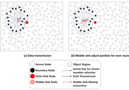
4.2.2 Static sink node outside the phenomena.
In this section, we will discuss the circumstance when static sink node is out of objects area, as shown in figure 2.
(c) Data transmission (d) Mobile sink adjust position for next round
Fig. 2 using twofold -sink approach in “static sink node outside the phenomena”
The proposed scheme appropriately adjust position of mobile sink node in accordance with this special case where the static sink node is situated outside the phenomenon. First with the information of boundary sensor nodes, we can obtain the object’s centroid using formula (2), as shown in figure 2(b). When the mobile sink moves to this point, it will broadcast hello message as mentioned in section 4.1. Subsequently, each boundary sensor node will receive this message and will compare its respective distances from the two sink nodes. The nearest sink node will be chosen as the destination for data transmissions during the current iteration.
5.
Performance evaluation
In this section, performance analysis of the proposed scheme, using twofold-sink approach, is presented. For comparisons, the proposed scheme is compared against single sink approach in terms of energy consumption and network lifetime.
5.1 Simulation setup
A 2-dimentional geographic plane of dimensions 1000 X 1000 m2 is considered for simulation test runs. Each discrete simulation test case is carried out 10 times in NS2 [14] using randomly generated seed values and the average value is plotted here. For each simulation run, 1000 sensor nodes are deployed randomly over the geographic plane, each having a sensing range of 20m. For simulations, it is assumed that the phenomena will only change as scattering of objects and will start from the centre of the geographical 2-D simulation plane.
5.2 Simulation results
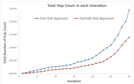
In simulation, we consider two conditions of the network: with single sink (static sink node) and with twofold sink (static sink node and mobile sink node) as shown in Fig 3., In proposed scheme, mobile sink participates to collect data from boundary sensor nodes in each iteration, which helps to reduce communication overhead. Because of mobile sink node number of hops count reduces as it moves and position itself adjacent the area of event. In Fig.3, it shows the comparison of hop-counts between one sink approach and twofold -sink approach. We can see when using twofold -sink approach, the number of hop counts obviously less compare to single static sink node approach. It is because in one static sink node approach, the boundary sensor nodes would send data at a long distance. In that process, the longer the distance, the more number of nodes are involved in the routing paths.
Fig. 3 Comparison of One sink and twofold-Sink approach in Total number of hop count in each round.
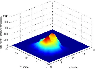
We divide the network 20x20 grids as shown in Fig. 4, whereas static sink node is in centroid location of the network and the initial phenomena appears close to the static sink node. We run the simulation for 20 iterations. At the end of simulation, we randomly select a single sensor node from each grid and calculated its number forwarded messages sent by it to static sink node. We can see that the high difference between of messages sent by sensor nodes near the static sink and the sensor nodes those are outlying. It is because most of event take place near the sink i.e. hello messages, boundary nodes selection, data gathering, whereas remaining network reposes in the idle mode.
Fig. 4 Total number of forward messages in single static approach.
Fig. 5 Total number of forward messages in twofold -Sink approach.
Total number of
forward messa
ges.
Total number of
forward messa
6.
Conclusion
This paper proposes a twofold -sink approach for boundary sensor node information colleting in continuous object tracking. It uses k-means algorithm to compute the optimal position for mobile sink to move, and with assistance of static sink node, it decrease data transmission, to extend the life time of network. Furthermore, We propose a solutions, considering two kinds of situation, static sink node inside and outside the phenomena. In Section 5, we shown performance analysis and simulation outcomes confirm our contentions. The results show that our proposed algorithm importantly surpasses the prior work as demonstrated in the simulations. Our future work will comprise precision of mobile sink’s movement and development of a new algorithm that reflects TTL value for mobile sink broadcasting.
References
1- CS Hussain, MS Park, AK Bashir, SC Shah, J Lee A collaborative scheme for boundary detection and tracking of continuous objects in WSNs - Intelligent Automation & Soft Computing, 2013.
2- Jung-Hwan K, Kee-Bum K, Chauhdary SH, Wencheng Y, Myong-Soon P (2008) DEMOCO: energy-efficient detection and monitoring for continuous objects in wireless sensor networks. IEICE Trans Commun 91:3648– 3656
3- Asmaa Ez-Zaidi and Said Rakrak, “A Comparative Study of Target Tracking Approaches in Wireless Sensor Networks,” Journal of Sensors, vol. 2016, Article ID 3270659, 11 pages, 2016. doi:10.1155/2016/3270659
4- X. B. Wu, G. H. Chen, “Dual-Sink: Using Static sink nodes for Lifetime Improvement in wireless sensor networks”, IEEE ICCCN, 13-16 Aug. 2007. pp. 1297-1302
5- J. Chen, M. B. Salim and M. Matsumoto, "Modeling the Energy Performance of Event-Driven Wireless Sensor Network by Using Static sink node and Mobile Sink," Sensors, vol. 10, no. 12, pp. 10876-10895, Dec 2010. Article (CrossRef Link).
6- X. Wu and G. Chen, "Dual-Sink: Using Mobile and Static sink nodes for Lifetime Improvement in Wireless Sensor Networks," in Proc. of the 16th International Conference on Computer Communications and Networks, pp. 1297-1302, Aug 2007. Article (CrossRef Link).
7- B. Wang, D. Xie, C. Chen, J. Ma and S. Cheng, "Deploying Multiple Mobile Sinks in Event-Driven WSNs," in Proc. of the IEEE International Conference on Communications, pp. 2293-2297, May 19-23, 2008. Article (CrossRef Link).
8- N. Bulusu, J. Heidemann, and D. Estrin, “GPS-less low cost outdoor location for very small devices”, Commun. (Special Issue on Smart Space and Environments), IEEE. Oct. 2000, vol. 7, pp. 28-34,
9- P.-K. Liao, M.-K. Chang, and C.-C. J. Kuo, “Distributed Edge Detection with Composite Hypothesis Test in Wireless Sensor Networks”, Communication Society Globecom, IEEE, 2004.
10- X. B. Wu, G. H. Chen, “Dual-Sink: Using Mobile and Static sink nodes for Lifetime Improvement in wireless sensor networks”, IEEE ICCCN, 13-16 Aug. 2007. pp. 1297-1302
11- R. Draves, J. Padhye, B. Zill “Routing in Multi-Radio, Multi-Hop Wireless Mesh Networks” MobiCom’04, ACM, Philadephia, Pennsylvania, USA, Sept 2004.
12- K-means algorithm: http://en.wikipedia.org/wiki/K-means_algorithm
13- Expectation-Maximization Algorithm:https://en.wikipedia.org/wiki/Expectation%E2%80%93maximization_algorithm