University of South Carolina
Scholar Commons
Theses and Dissertations
2016
Utilization Of Satellite-Derived Salinity For ENSO
Studies And Climate Indices
Caroline Mary Corbett University of South Carolina
Follow this and additional works at:https://scholarcommons.sc.edu/etd Part of theGeology Commons
This Open Access Thesis is brought to you by Scholar Commons. It has been accepted for inclusion in Theses and Dissertations by an authorized administrator of Scholar Commons. For more information, please [email protected].
Recommended Citation
Corbett, C. M.(2016).Utilization Of Satellite-Derived Salinity For ENSO Studies And Climate Indices.(Master's thesis). Retrieved from
UTILIZATION OF SATELLITE-DERIVED SALINITY FOR ENSO
STUDIES AND CLIMATE INDICES
by
Caroline Mary Corbett
Bachelor of Science Saint Louis University, 2015
Submitted in Partial Fulfillment of the Requirements
For the Degree of Master of Science in
Geological Sciences
College of Arts and Sciences
University of South Carolina
2016
Accepted by:
Subrahmanyam Bulusu, Director of Thesis
Venkat Lakshmi, Reader
Alexander Yankovsky, Reader
Camelia Knapp, Reader
ACKNOWLEGEMENTS
This thesis was supported in part by NASA’s Physical Oceanography Program.
This work would not have been possible without the support of numerous people. I would
first like to extend my thanks to my major professor, Prof. Subrahmanyam Bulusu, for his
generosity, guidance, motivation, and confidence in my abilities throughout my academic
career at USC. Secondly, I would like to thank my committee members, Prof. Venkat
Lakshmi, Dr. Alexander Yankovsky, and Prof. Camelia Knapp, for their time and
expertise. I would also like to thank my lab mates Joseph D’Addezio, Bryce Melzer,
Jessica Burns, Brady Ferster, and Corinne Trott for their constant personal and academic
support. And lastly, I would like to acknowledge my parents and sister, as well as my
partner Kevin Tormasi and his family for their boundless emotional, intellectual, and
ABSTRACT
Conventionally, El Niño-Southern Oscillation (ENSO) is studied using sea
surface temperature (SST) observations in the central and eastern equatorial Pacific
Ocean. Recently, sea surface salinity (SSS) in the equatorial Pacific has been studied in
relation to the phases of ENSO. Previously, SSS was observed in the equatorial Pacific
using the Tropical Ocean Global Atmosphere (TOGA) / Tropical Atmosphere Ocean
(TOA), the Argo float network, and Oceanic General Circulation Models (OGCM). The
launch of NASA’s Aquarius Salinity Mission and ESA’s Soil Moisture Ocean Salinity
(SMOS) opened a new era in which high resolution global near real-time SSS
observations are readily available. These satellites have made the collection and analysis
of SSS data easier and have improved our understanding of salinity variability during
ENSO.
This study examines the accuracy and validity of the Aquarius and SMOS SSS
datasets and compares them to the Argo float observations. This comparison shows that
the three datasets are comparable, although there are some discrepancies. These
differences are mainly focused in the regions of upwelling and high precipitation. The
performance of these datasets is analyzed specifically during the 2014-15 ENSO event.
Their observations are comparable during this event, but there are notable differences.
These salinity discrepancies cannot be explained with evaporation and precipitation
Further examination of the 2014-15 ENSO event is conducted, and it is compared
to the strong 1997-98 El Niño event and the similarly failed 2012-13 ENSO event. This
study demonstrates that both E-P variability and anomalously eastward surface currents
are required for the full development of El Niño conditions. It is also essential that
anomalous fresh SSS migrate eastward of the International Date Line in order for a
successful El Niño to occur. Observed SSS variability in the equatorial Pacific is clearly
linked to the onset and death of El Niño conditions.
Finally, a new index called the Western Pacific Salinity Index (WPSI) is
developed based on the SSS variability observed in the region defined from 5°N to 5°S
and 160°E to 170°W. When calculated using Argo and SMOS SSS data, this index is
capable of identifying warm, cool, and neutral phases of ENSO. However, the Aquarius
dataset is less capable of observing the phases of ENSO. WPSI is highly correlated to
TABLE OF CONTENTS
ACKNOWLEGEMENTS ... iii
ABSTRACT ... iv
LIST OF TABLES ... viii
LIST OF FIGURES ... ix
CHAPTER 1. INTRODUCTION ...1
1.1 STUDY AREA ...1
1.2 EL NIÑO-SOUTHERN OSCILLATION ...1
1.3 SEA SURFACE SALINITY ...2
CHAPTER 2. VALIDATION OF SATELLITE-DERIVED SALINITY IN THE EQUATORIAL PACIFIC WITH SPECIFIC EMPHASIS ON THE 2014-15 ENSO EVENT ...5
2.1 INTRODUCTION ...6
2.2 DATA AND METHODS ...8
2.3 RESULTS ...10
2.4 CONCLUSION ...13
CHAPTER 3. A COMPARISON OF SEA SURFACE SALINITY IN THE EQUATORIAL PACIFIC OCEAN DURING HE 1997-98, 2012-13, AND 2014-15 ENSO EVENTS ...23
3.1 INTRODUCTION ...24
3.2 MATERIALS AND METHODOLOGY ...26
3.3 RESULTS ...29
4.1 SUMMARY ...49
4.2 WESTERN PACIFIC SALINITY INDEX ...50
REFERENCES ...57
APPENDIX A. COPYRIGHT PERMISSIONS ...65
LIST OF TABLES
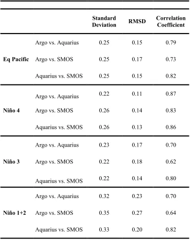
Table 2.1. Comparison of the Argo, Aquarius, and SMOS anomalies with respect to the mean taken from August 2011 to May 2015 in the equatorial Pacific (5°N-5°S, 130°E-90°W), Niño 4 region (5°N-(5°N-5°S, 160°E-150°W), Niño 3 region (5°N-5°S, 150°-90°W), and Niño 1 + 2 region (0°-10°S, 90°-80°W) ...16
Table 3.1. Comparison of SODA 1997-98 Argo 2012-13, and Argo 2014-15 SSS anomalies (black, blue, and red respectively in Fig. 3.5) in each of the Niño boxes ...39
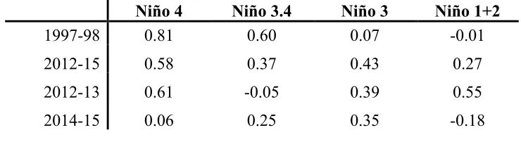
Table 3.2. Correlation coefficients between E-P and SSS anomalies in each of the Niño boxes in 1997-98 (Fig. 3.7), 2012-15, 2012-13, and 2014-15 (Fig. 3.8) ...40
Table 4.1 Phases of ENSO from 2005 to 2016 as defined by Japan Meteorological Agency Index (JMA), Oceanic Niño Index (ONI) and the Niño 3.4 Index ...53
LIST OF FIGURES
Figure 2.1. Mean SSS (psu) from August 2011 to May 2015 for (A) Argo and (B) Aquarius and (C) SMOS. Difference in mean SSS (psu) for (D) Argo and Aquarius, (E) Argo and SMOS, and (F) Aquarius and SMOS ...17
Figure 2.2. Mean (a) evaporation, (b) precipitation, and (c) E–P from monthly ECMWF evaporation and precipitation (mm) for the period from August 2011 to May 2015...18
Figure 2.3. (Top Row) SSS variability from Argo (blue), Aquarius (red), and SMOS (green) averaged over (A) equatorial Pacific (5°N-5°S, 130°E-90°W), (B) Niño 4 region (5°N-5°S, 160°E-150°W), (C) Niño 3 region (5°N-5°S, 150°-90°W), and (D) Niño 1 + 2 region (0°-10°S, 90°-80°W). (Bottom Row)
monthly SSS anomalies ...19
Figure 2.4. Taylor diagrams comparing Aquarius and SMOS SSS anomalies with Argo SSS anomalies with respect to the mean taken from August 2011 to May 2015 in the equatorial Pacific (5°N-5°S, 130°E-90°W), the Niño 4 region (5°N-5°S, 160°E-150°W), the Niño 3 region (5°N-5°S, 150°-90°W) and the Niño 1 + 2 region (0°-10°S, 90°-80°W) ...20
Figure 2.5. SSS anomalies (psu) from April 2014 to February 2015 using Argo (left column), Aquarius (center column), and SMOS (right column). Anomalous OSCAR surface currents (m s-1) for the same month are shown in the black arrows ...21
Figure 2.6. Anomalous monthly ECMWF E–P (mm) from April 2014 to February 2015...22
Figure 3.1. Hovmöller diagram from 130°E to 90°W and averaged over 5°N – 5°S of ECMWF 5-day zonal winds (m s-1) for (A) January 1996–December 1998, (B) January 2011–December 2013, and (C) January 2013–December 2015. The black line represents the location of the International Date Line ...41
Figure 3.3. Same as Fig. 3.1 but for SSS anomalies (psu) using (A) SODA reanalysis and (B, C) Argo ...43
Figure 3.4. Plot of the regions defined as Niño 4, Niño 3.4, Niño 3, and Niño 1+2. Niño 4 is the region from 5°N–5°S, 160°E–150°W (shaded in blue). Niño 3.4 is the region from 5°N–5°S, 170°W–120°W (shaded in green). Niño 3 is the region from 5°N–5°S, 150°W–90°W (shaded in red). Niño 1+2 is the region from 0°–10°S, 90°W–80°W ...44
Figure 3.5. Seasonal variability of SSS anomalies (psu) in each of the Niño boxes from SODA (January 1997–December 1998) (black line) and Argo (January 2012– December 2013, January 2014–December 2014) (blue line, red line
respectively). Solid black line represents zero ...45
Figure 3.6. Same as Fig. 3.1 but for anomalous E–P (mm/day) using OA Flux
evaporation and (A) GPCP precipitation, (B, C) TRMM precipitation ...46
Figure 3.7. Seasonal variability of SODA SSS anomalies (psu) (black line and y-axis) and anomalous E–P (mm/day) using OA Flux evaporation and GPCP precipitation (blue line and y-axis) for each of the Niño boxes from January 1997–December 1998. The black line represents zero ...47
Figure 3.8. Same as Fig. 3.7 but for January 2012–December 2015 using Argo SSS anomalies (psu), and anomalous E–P (mm/day) using OA Flux evaporation and TRMM precipitation ...48
Figure 4.1 Proposed WPSI box from 5°N to 5°S and 160°E to 170°W ...55
CHAPTER 1
INTRODUCTION
1.1STUDY AREA
The equatorial Pacific Ocean is the focus study area for this research. This region
is generally defined from 5°N to 5°S, 120°E to 70°W, a region which is diverse in sea
surface temperature (SST) and sea surface salinity (SSS). The western Pacific warm pool
dominates the western equatorial Pacific. Convection over the warm SSTs of the western
Pacific warm pool causes large amounts of precipitation over the region (Delcroix et al.,
1996; Chen et al., 2004; Cravatte et al., 2009); therefore, this region is also characterized
by fresh SSS (Cravatte et al., 2009; Qu et al., 2014).
The eastern equatorial Pacific is dominated by cool SSTs, higher saline, and
nutrient rich waters; this is due to upwelling off the coast of South America (Chavez et
al., 1999). Although these are the mean conditions in the equatorial Pacific Ocean, they
are altered significantly during El Niño-Southern Oscillation.
1.2EL NIÑO-SOUTHERN OSCILLATION
El Niño-Southern Oscillation (ENSO) is a climate scale phenomena that occurs in
the equatorial Pacific Ocean and has global oceanic and atmospheric impacts (Singh et
al., 2011; Menkes et al., 2014; Capotondi et al., 2015; McPhaden, 2015). ENSO has three
During El Niño, warm SSTs from the western Pacific warm pool are zonally
displaced eastward (Trenberth, 1997; Singh et al., 2011; Qu and Yu, 2014). Anomalously
warm SSTs migrate to the coast of South America, cutting off the equatorial upwelling
that occurs in the region (Trenberth, 1997). This affects the nutrient supply and severely
impacts biological processes and diversity (Trenberth, 1997; Chavez et al., 1999). In the
atmosphere during El Niño, the Hadley and Walker cells are altered. This causes
anomalously high precipitation over the western and central Pacific. Additional
atmospheric changes occur globally and the effects are observed in regions such as North
America and Africa. Furthermore, El Niño conditions are linked to high sea surface
height (SSH) observations in the eastern equatorial Pacific and linked to equatorial
Kelvin Wave patterns (Picaut and Delcroix, 1995; Picaut et al., 2002).
Oppositely, during La Niña, anomalously warm SSTs migrate westward and the
eastern equatorial Pacific is dominated by an anomalously large equatorial Pacific “cold
tongue” (Hasson et al., 2014). This region is nutrient rich, fueled by increased upwelling
off the coast of South America (Chavez, 1999; Hasson et al., 2014). The Walker
Circulation is altered during La Niña conditions, which affects the precipitation patterns
in the western Pacific (Hasson et al., 2014). Additionally, La Niña conditions are linked
to Rossby Wave patterns (Picaut and Delcroix, 1995; Picaut et al., 2002).
1.3SEA SURFACE SALINITY
ENSO is usually observed using SSH and SST anomalies throughout the
and cool phases of ENSO. A number of new mechanisms for SSS measurement allow for
easier, more extensive, and long-term analysis of the SSS variability.
SSS is an important variable to study generally and in connection to El Niño. SSS
can be used as a proxy for evaporation minus precipitation (E-P), because SSS increases
when evaporation dominates and SSS decreases when precipitation dominates (Yu,
2011). Unlike SST, SSS is unaffected by the diurnal cycle and varies at a slower
timescale (Spall, 1992; Yu, 2011; Qu and Yu, 2014).
SSS during ENSO is not well understood but has been studied more with
increasing access to global and high-resolution measurements. The launch of NASA’s
Aquarius Salinity Mission and ESA’s Soil Moisture Ocean Salinity (SMOS) have
provided global satellite derived SSS data since 2010. In association with the expansive
Argo float network and oceanic models, these satellite observations can be used to
expand our understanding of SSS variability.
Chapter 2 validates the use of Aquarius and SMOS SSS data as compared to Argo
near-surface salinity data in the equatorial Pacific generally and during the 2014-15
ENSO event. This study reveals the biases of both satellites as compared to Argo and
shows that the satellites are comparable in this region. However, the Aquarius Mission
ended in June 2015, leaving SMOS as the most useful satellite tool still in operation for
the study of SSS in the equatorial Pacific during ENSO.
Chapter 3 is a comparison study of the strong 1997-98 El Niño, and the failed
2012-13 and 2014-15 ENSO events. This study identifies the importance of and need for
both anomalous E-P and anomalous surface currents in the SSS variability to initiate a
factor in the failure of the 2012-13 and 2014-15 ENSO events. Additionally, the
International Date Line is identified as an important marker, as anomalously fresh SSS
must migrate east of it during a fully formed and long lasting El Niño event.
Lastly, Chapter 4 summarizes the major findings of this work. The use of these
findings for future research into and development of SSS ENSO indices is presented and
discussed. The findings from Chapters 2 and 3 can be implemented into SSS indices for
ENSO forecasts. A new SSS ENSO index called the Western Pacific Salinity Index
(WPSI) is introduced. The calculation of the index is conducted using the Argo,
Aquarius, and SMOS datasets. WPSI is shown to be capable of identifying the three
CHAPTER 2
VALIDATION OF SATELLITE-DERIVED SALINITY IN THE EQUATORIAL
PACIFIC WITH SPECIFIC EMPHASIS ON THE 2014-15 ENSO EVENT1
1Corbett, C.M. and B. Subrahmanyam. 2016. IEEE Geosci. Remote Sens Lett.
doi:10.1109/LGRS.2016.2619980.
ABSTRACT
This letter compares satellite and in situ sea surface salinity (SSS) measurements
in the tropical Pacific Ocean and validates the performance of satellite products during
the 2014–15 El Niño-Southern Oscillation (ENSO) event. SSS measurements from
NASA’s Aquarius Salinity Mission and the European Space Agency’s Soil Moisture and
Ocean Salinity (SMOS) are compared with Argo float data. This comparison shows that
the Aquarius and SMOS satellites are generally able to resolve the SSS in the tropical
Pacific, despite some discrepancies in regions of upwelling and high precipitation. The
two satellites perform better with respect to Argo in Niño 4 than in Niño 3 and Niño 1 +
2. However, in each region, Aquarius and SMOS are highly correlated with each other.
During the 2014–15 ENSO event, each dataset observes similar SSS, although some
discrepancies exist. Analysis of anomalous evaporation minus precipitation during this
event demonstrates that the differences between each dataset are not fully explained by
precipitation patterns.
2.1 INTRODUCTION
Salinity variability is known to play an important role in ocean dynamics (Rao
and Sivakumar, 2003; Foltz and McPhaden, 2008; Yu, 2011; Bingham et al., 2012). Sea
surface and near surface salinity variability is closely related to evaporation minus
dominates the intertropical convergence zone (ITCZ) and the South Pacific convergence
zone (SPCZ). These two regions meet in the western equatorial Pacific, at the western
Pacific warm pool. Low sea surface salinity (SSS) is found along the ITCZ, SPCZ, and in
the western Pacific warm pool due to the rainfall in these regions (Delcroix et al., 1996;
Vialard et al., 2002; Yu, 2011; Qu et al., 2014).
SSS and E-P in the tropical Pacific are altered during the phases of El
Niño-Southern Oscillation (ENSO). The western Pacific warm pool and the associated fresh
pool are zonally displaced eastward during El Niño (Trenberth, 1997; Singh et al., 2011).
Changes in the Walker and Hadley cells during ENSO cause anomalously high
precipitation over the western and central Pacific (Lau and Chan, 1983; Delcroix et al.,
1996). Understanding SSS variability during El Niño is important for the
ocean-atmosphere coupling during events. SSS and thus salinity stratification are partially
affected by anomalous E-P patterns in the tropical Pacific. Salinity stratification and
barrier layer formation are understood to greatly influence El Niño formation (Maes et
al., 2002; Maes et al., 2004; Qu et al., 2014).
Until recently, global SSS measurements have been sparse. The Argo float
network provides global near surface salinity measurements throughout the oceans.
However, float population is scarce in many areas around the world. With the launch of
NASA’s Aquarius Salinity Mission, which ended June 7, 2015, and the European Space
Agency’s Soil Moisture Ocean Salinity (SMOS), which is still operational, global
high-resolution SSS data is now more readily available. Argo, Aquarius, and SMOS salinity
In this letter, we compare the Argo, Aquarius and SMOS SSS data sets and their
performance in the tropical Pacific. Specifically, the performance of the two satellites is
assessed in comparison to Argo during the 2014–15 El Niño. The unusual progression of
this event makes it an interesting case study for satellite validation. The results of this
letter aim to assess the validity of the Aquarius and SMOS data sets in the tropical Pacific
generally and during El Niño events. We also aim to advance our understanding of the
SSS variability during the irregular 2014–15 El Niño event.
2.2 DATA AND METHODS
In this letter, we use International Pacific Research Center processed monthly
Argo SSS data obtained from the Asia-Pacific Data-Research Center
(http://apdrc.soest.hawaii.edu/projects/argo/). These data are produced by optimal
interpolation with a spatial resolution of 1° × 1° and are available from January 2005 to
June 2016. We use monthly Aquarius version 4.0 Level 3 SSS data at a 1° × 1° spatial
resolution obtained from NASA Jet Propulsion Laboratory (JPL) Physical Oceanography
Distributed Active Archive Center (PO.DAAC) (http://podaac.jpl.nasa.gov/aquarius).
The Aquarius mission ended in June 2015 and the monthly data set is available from
August 2011 to May 2015. SMOS version 2.0 Level 3 monthly SSS data at a 0.25° ×
0.25° spatial resolution is used and obtained from Barcelona Expert Centre (http://
cp34-bec.cmima.csic.es/). These data are available from January 2010 to June 2016, although
the mission is still in operation. Olmedo et al., (2016) provide detailed information about
methods by which this product was processed. For comparisons with Argo and Aquarius,
We use evaporation and precipitation data from the European Centre for
Medium-Range Weather Forecasts (ECMWF) ERA-Interim global atmospheric reanalysis
(http://apps.ecmwf.int/datasets/data/interim-fullmnth/levtype=sfc/). These data are
synoptic monthly means at a 1° × 1° spatial resolution and are available from January
1979 to April 2016. For surface currents, we use the Ocean Surface Current Analyses
Real-time (OSCAR) at a 0.33° × 0.33° spatial resolution, which is available through
NASA JPL PO.DAAC. These data are available from October 1992 to December 2015 in
a 5-day cycle format. For this letter, we converted to a monthly format and reduced the
spatial resolution to 1° × 1° to match the salinity data sets.
From August 2011 to May 2015, Argo, Aquarius, and SMOS were all operational.
This time period is used for comparison and statistical analysis of the three data sets. For
each data set, anomalies are calculated by removing the monthly means. Monthly means
are calculated by averaging monthly data over the entire span on the data set.
It is important to discuss the differences between Argo in situ measurements and
satellite products before conducting the validation. Argo floats measure salinity from 5 to
2000 m depth and measurements are not taken above 5 m (Moon et al., 2014; Qu et al.,
2014; Song et al., 2015). Therefore, Argo SSS is more accurately described as
near-surface salinity measurements (Lagerloef et al., 2008; Riser et al., 2008; Henocq et al.,
2010; Boutin et al., 2013; Qu et al., 2014). On the other hand, satellites observe skin
measurements of salinity, which is approximately equal to the top 5 cm of the ocean
(Moon et al., 2014; Song et al., 2015). Surface and near-surface salinity can vary
significantly. This is most notably due to rainfall-induced surface freshwater pooling
et al., 2014; Song et al., 2015). Therefore, discrepancies in the data sets can arise from the
differences in measurement depth. Additional causes for error are discussed later.
2.3 RESULTS
2.3.1 ASSESSMENT OF AQUARIUS AND SMOS
To assess the validity of Aquarius and SMOS SSS in the tropical Pacific, we
compare them to Argo. Generally, the three data sets observe the same mean SSS (Figure
2.1). Subtle differences between the data sets are realized when the satellite data sets are
subtracted from Argo and when SMOS is subtracted from Aquarius.
Argo has a salty bias, greater than 0.45 psu, along the ITCZ over the region. As
discussed, satellites are affected by precipitation induced surface freshwater pooling
because they measure the top 5 cm of the ocean surface. Alternatively, Argo profilers
measure at 5 m depth and SSS is extrapolated to the surface (Lagerloef et al., 2008; Riser
et al., 2008; Henocq et al., 2010; Boutin et al., 2013; Qu et al., 2014). Compared to
Aquarius, Argo has a salty bias off the coast of Panama (Figure 2.1D). Argo has a salty
bias over SMOS off the coast of Panama and much of South America (Figure 2.1E).
Argo has a fresh bias of the order of −0.55 psu along the rest of the Central American
coastline (Figure 2.1D, E). Land contamination and the scarcity of Argo floats in this
region could be contributing to this.
Aquarius has a small salt bias off Peru (Figure 2.1D). SMOS has a larger salt bias,
of the order of 0.35 psu, along the equator from 140° W to the coast of South America
(Figure 2.1E). Compared to Aquarius, SMOS has a fresh bias along the coast of Central
contamination (Figure 2.1F). SMOS also has a fresh bias along portions of the ITCZ and
SPCZ. SMOS has a salt bias along the equator, which is likely due to upwelling (Qu et
al., 2014). This SMOS salt bias is also documented by (Maes et al., 2014).
Evaporation and precipitation patterns in Figure 2.2 match results found in
Delcroix et al., (1996), Vialard et al., (2002), Yu, (2011), and Qu et al., (2014). Negative
E-P, resulting from more precipitation than evaporation, occurs along the ITCZ and
SPCZ and over the western Pacific warm pool. Significant E-P anomalies occur along the
coast of Panama, Columbia, and Ecuador. This is the region where Argo observes saltier
salinities than the satellites. Near zero and weakly positive E-P occurs along the equator,
where SMOS observes saltier salinities than Argo and Aquarius.
Argo and Aquarius appear to measure similar SSS in the equatorial Pacific, Niño
4 and Niño 3 (Figure 2.3A, B, C). SMOS observes fresher SSS in the equatorial Pacific
and Niño 4, but is similar to Argo and Aquarius in Niño 3. However, all three data sets
agree on the general trends of SSS in these regions. In Niño 4, all data sets agree on the
steepness and timing of the decrease in SSS in early 2014. Less agreement occurs in Niño
1 + 2, where SMOS again observes fresher SSS (Figure 2.3D). SSS anomalies appear to
correlate well in each of the regions (Figure 2.3E-H). Discrepancies that exist are on the
order of 0.2 psu or less. The largest differences between anomalies are seen in Niño 1 +
2.
Statistical analysis of Argo, Aquarius and SMOS anomalies was performed
(Table 2.1, Figure 2.4). Aquarius consistently performs better than SMOS when
compared to Argo. The lowest standard deviations and root-mean-square deviations
Pacific and Niño 4. Compared to the other regions, the satellites perform poorly with
respect to Argo in Niño 3 and Niño 1 + 2. For each comparison, the largest standard
deviations and RMSDs are in Niño 1 + 2. These results indicate that Aquarius and Argo
are most similar across the Pacific, but SMOS is still comparable.
2.3.2 SEA SURFACE SALINITY DURING THE 2014-15 ENSO EVENT
The 2014–15 El Niño is rather distinctive. In early 2014, a strong El Niño was
forecasted but failed to fully form. In 2015, the El Niño unexpectedly regenerated and
became one of the strongest El Niño events on record (McPhaden, 2015). The stalling in
2014 and the regeneration of the El Niño in 2015 make the progression of this event
unique.
During this event, Argo, Aquarius, and SMOS appear to observe similar SSS
(Figure 2.5). All three data sets tend to agree on the location of negative and positive
anomalies. Argo tends to see larger regions of negative and positive anomalies than
Aquarius. SMOS tends to show more detail and observes fresher anomalies in the regions
of negative anomalies. The largest discrepancies between the data sets are found in the
ITCZ, SPCZ, and off the coast of Central and South America. This coincides with
discrepancies between datasets in Figure 2.1.
Correlations between Argo, Aquarius, and SMOS during each month in the
tropical Pacific are calculated but not shown. Statistically, Argo is minimally correlated
with Aquarius and SMOS (less than 0.28 correlation coefficient) during each month.
Errors during this event are calculated in the equatorial Pacific, Niño 4, Niño 3,
and Niño 1 + 2 regions but also not shown. In each of the regions, the data sets are less
correlated during this event than they are from August 2011 to May 2015 (Table 2.1,
Figure 2.4). All data sets are strongly correlated in the equatorial Pacific, and Niño 4 and
weakly correlated in Niño 3. In Niño 1 + 2, only Aquarius and SMOS are strongly
correlated and the satellite data sets are not correlated to Argo.
Negative E-P anomalies over the ITCZ and SPCZ vary throughout the event but
can generally explain the observed SSS differences (Figure 2.6). Positive E-P anomalies
tend to dominate along the equator, where the three data sets are strongly correlated in
Niño 4. This indicates that the three data sets perform well with respect to each other due
to the lack of precipitation.
Negative E-P anomalies near Panama, Columbia, and Ecuador cannot explain the
observed SSS discrepancies, as Argo tends to observe fresher anomalies. Near normal
conditions and weakly positive E-P anomalies are seen in Niño 3 and Niño 1 + 2; SSS
discrepancies and lack of correlation are likely explained by upwelling conditions in and
around this region.
2.4 CONCLUSION
The modification and role of SSS in the tropical Pacific during El Niño is
increasingly studied. Atmospheric and oceanic changes during El Niño alter SSS patterns
and E-P throughout the tropical Pacific. Understanding this SSS variability is important
for characterizing the dynamical changes that occur during these events. Satellite
we have compared Aquarius and SMOS to Argo to validate the accuracy of the salinity
data sets in the tropical Pacific. We then examined their performance specifically during
the unique 2014–15 El Niño event. E-P variability was assessed as a possible cause for
the disagreements between data sets.
Typically, satellites observe fresher anomalies than Argo in regions of significant
precipitation. This was found to be true over much of the ITCZ and SPCZ, where Argo
has a salty bias. Significant negative E-P along the coast of Panama, Columbia, and
Ecuador explain the satellite fresh bias. The satellites have a salt bias over the region of
upwelling off the Peruvian coast.
When using these data sets to study the 2014–15 El Niño, these biases are
important to note. SSS discrepancies between Argo, Aquarius, and SMOS during this
event most notably occur in the ITCZ, SPCZ, and off the coast of Central and South
America. Anomalous E-P cannot always explain these salinity differences.
In the ITCZ and SPCZ, anomalously negative E-P can explain SSS discrepancies.
However, anomalously negative E-P is seen off the coast of Panama, where Argo
observes more negative SSS anomalies than the satellites. Near normal and slightly
positive E-P anomalies are observed in the Niño 3 and Niño 1 + 2 regions, despite a lack
of correlation between Argo and the satellites. Therefore, precipitation patterns cannot
completely reconcile the disagreements between data sets. Consequently, differences
between Argo and satellite observations must be discussed and taken into account.
There are numerous possible explanations for disagreements between Argo and
satellite observations. The first is the depth sampling differences between Argo and
satellites observe salinity in the top 5 cm. Differences in surface and subsurface SSS
variability caused by freshwater fluxes may be driving the discrepancies between Argo
and satellite observations (Moon et al., 2014; Song et al., 2015). Second, the relatively
coarse Argo observations, compared to satellites, and the differences in sampling times
between the products may also factor into the differences (Boutin et al., 2016). Land
contamination from satellite observations in the Niño 1 + 2 region may also factor into
the observed discrepancies.
Overall, the comparisons between the three data sets are favorable. Argo,
Aquarius, and SMOS generally agree on the large scale SSS patterns in the equatorial
Pacific. However, the biases are important to take into account when analyzing smaller
regions, specifically along the ITCZ, SPCZ, and the coast of Central and South America.
During El Niño, the data sets are still strongly correlated, but disagreements become
problematic when observing SSS in the eastern Niño regions.
As the SMOS mission continues its operation, additional studies of SSS
variability in the equatorial Pacific can be conducted. Future El Niño events can be
studied in detail using Argo, SMOS, and the new Soil Moisture Active Passive (SMAP)
Table 2.1. Comparison of the Argo, Aquarius, and SMOS anomalies with respect to the mean taken from August 2011 to May 2015 in the equatorial Pacific (5°N-5°S, 130°E-90°W), Niño 4 region (5°N-5°S, 160°E-150°W), Niño 3 region (5°N-5°S, 150°-130°E-90°W), and Niño 1 + 2 region (0°-10°S, 90°-80°W)
Standard
Deviation RMSD Correlation Coefficient
Argo vs. Aquarius 0.25 0.15 0.79
Eq Pacific Argo vs. SMOS 0.25 0.17 0.73
Aquarius vs. SMOS 0.25 0.15 0.82
Argo vs. Aquarius 0.22 0.11 0.87
Niño 4 Argo vs. SMOS 0.26 0.14 0.83
Aquarius vs. SMOS 0.26 0.13 0.86
Argo vs. Aquarius 0.23 0.17 0.70
Niño 3 Argo vs. SMOS 0.22 0.18 0.62
Aquarius vs. SMOS 0.22 0.14 0.80
Argo vs. Aquarius 0.32 0.23 0.70
Niño 1+2 Argo vs. SMOS 0.35 0.27 0.64
CHAPTER 3
A COMPARISON OF SEA SURFACE SALINITY IN THE EQUATORIAL PACIFIC
OCEAN DURING THE 1997-98, 2012-13, AND 2014-15 ENSO EVENTS2
ABSTRACT
This study examines and compares the sea surface salinity (SSS) variability
during the 1997-98 El Niño event and the failed 2012-13 and 2014-15 El Niño events.
Our analysis utilizes salinity data from Argo observations and the Simple Ocean Data
Assimilation (SODA) reanalysis to examine the SSS variability. Advective processes and
evaporation minus precipitation (E-P) variability is understood to influence SSS
variability. Using surface wind, surface current, evaporation, and precipitation data, we
analyze the causes for the observed SSS variability during each event. This comparison
study demonstrates the importance of both advective processes and E-P variability during
the generation and onset of a successful El Niño, while a lack of one or both of these
processes leads to a failed ENSO event.
3.1 INTRODUCTION
El Niño-Southern Oscillation (ENSO) is an important climatic phenomenon that
occurs in the equatorial Pacific Ocean and has local and global implications on weather
and biology (Singh et al., 2011; Menkes et al., 2014; Capotondi et al., 2015; McPhaden,
2015). While ENSO involves ocean-atmosphere interactions, it generally includes a zonal
displacement of the western Pacific warm pool (Trenberth, 1997; Qu and Yu, 2014). The
zonal displacement eastward represents the warm, or positive, phase of ENSO, called El
Conventionally, the phases of ENSO are observed and studied using SST
anomalies. Recently, El Niño is being studied by examining sea surface salinity (SSS),
surface winds and currents, and sea surface height (SSH) variability (Taft and Kessler,
1991; Li and Clarke, 1994; McPhaden, 1999; Johnson et al., 2000; Menkes et al., 2014).
Lack of extensive and accurate data previously hindered our ability to fully study
and understand the connection between SSS variability and ENSO. The Tropical Ocean
Global Atmosphere (TOGA)/Tropical Atmosphere Ocean (TOA) mooring project
provides in-situ SSS observations across the equatorial Pacific, although the coverage is
relatively sparse. SSS data is more readily available with the widespread Argo float
network, which has been in operation since 2005. The Simple Ocean Data Assimilation
(SODA) reanalysis provides a long-term SSS reanalysis dataset. With long-term and
global datasets, SSS data can be examined more thoroughly in connection to El Niño
events.
Studying SSS provides a new perspective and an alternative mechanism for
viewing and forecasting ENSO. SSS variability during ENSO events has numerous
causes and can be influenced by both atmospheric and oceanic dynamics and processes.
Advective processes, caused by wind and current variations, and evaporation and
precipitation patterns are the two important forcings for SSS variability focused on in this
paper.
Westerly Wind Burst (WWB) events, or the slackening and reversal of the Pacific
trade winds, affect the direction of surface currents (Menkes et al., 2014). WWB events
are highly variable in their duration, but typically last between 5 and 20 days (Harrison
current pattern; often, the anomalous surface current pattern lasts longer than the duration
of the WWB event (Giese and Harrison, 1990). For the remainder of this paper, it is
assumed that anomalously eastward currents are, at least partially, generated by WWB
events. Eastward currents throughout the Pacific act to advect the fresh waters of the
western Pacific warm pool eastward.
Evaporation and precipitation patterns, specifically E-P, across the Pacific also
affect SSS variability. The western Pacific warm pool is characterized by fresh surface
waters due to increased convection and precipitation over the region (Delcroix et al.,
1996; Chen et al., 2004; Cravatte et al., 2009). Evaporation and precipitation variability is
more significant in the eastern Pacific and greatly influences SSS variability in this
region (Delcroix et al., 1996). During ENSO changes in the Walker Circulation cause
higher than normal precipitation patterns in the western and central Pacific (Lau et al.,
1983; Delcroix et al., 1996).
In this study, we compare the 1997-98, 2012-13, and 2014-15 ENSO events to
better understand their similarities and differences. Surface winds, surface currents, and
evaporation and precipitation patterns are examined to gain a full understanding of their
influences on SSS variability during each event. The results of this study aim to advance
our understanding of SSS variability during El Niño. We also aim to better characterize
the conditions that aided in the development of the 1997-98 El Niño and the conditions
3.2 MATERIALS AND METHODOLOGY
3.2.1 DATA SOURCES
The International Pacific Research Center (IPRC) processed monthly SSS Argo
dataset is available through the Asian Pacific Data Research Center (APDRC). These
data are optimally interpolated with a spatial resolution of 1°x1° and available from
January 2005 to June 2016. It is important to note that Argo floats measure salinity from
5m to 2,000m depth and this product does not extrapolate the salinity measurement to the
surface; therefore the surface salinity measurement used is taken at 5m depth (Moon and
Song, 2014; Qu et al., 2014; Song et al., 2015). Lebedev et al., (2007) provides additional
information about the methods by which this product is created. SSS anomalies are
calculated by removing the monthly means averaged from January 2005 to June 2016.
The Ocean Surface Current Analyses Real-time (OSCAR) uses satellite SSH,
wind, and temperature data to estimate zonal and meridional surface currents at a
0.33°x0.33° spatial resolution. The data are output in a 5-day cycle format and available
through NASA JPL Physical Oceanography Distributed Active Archive Center
(PO.DAAC) from October 1992 to December 2015. For this research, the surface current
u- and v- components are averaged for each month and the spatial resolution is reduced to
a 1°x1° for comparison with other datasets. Anomalies are calculated by removing the
monthly means, which are calculated from October 1992 to December 2015.
The Objectively Analyzed Air-Sea Fluxes (OA Flux) project conducted by the
Woods Hole Oceanographic Institution provides monthly ocean evaporation data from
mm/day and anomalies are calculated by removing the monthly means averaged from
January 1958 to September 2015.
NASA Goddard Space Flight Center (GSFC) provides the Tropical Rainfall
Measuring Mission (TRMM)-adjusted merged infrared (IR) precipitation data (Product
3B42). Kummerow et al., (1998, 2000) describe the TRMM project and this merged
product. The data are available at a 0.25°x0.25° spatial resolution and a 3-hr timescale
from January 2000 to August 2015. For comparison with other datasets, the spatial
resolution is reduced to 1°x1° and averaged by month. Anomalies are calculated by
removing climatology calculated from January 2000 to August 2015.
Global Precipitation Climatology Project (GPCP), provided by NASA GSFC,
utilizes data from satellites, rain gauges, and sounding observations to estimate monthly
global rainfall totals from January 1979 to October 2015 at a 2.5°x2.5° spatial resolution.
Adler et al., (2003) provide a complete explanation of the dataset. For comparison with
TRMM, the data are interpolated to a 1°x1° spatial resolution and monthly anomalies are
calculated by removing the monthly means from January 1979 to October 2015. This
dataset supplements the TRMM data to study years prior to 2000.
3.2.2 REANALYSIS PRODUCTS
The Simple Ocean Data Assimilation (SODA) reanalysis is an ocean reanalysis
system. The version 2.2.4 monthly averaged salinity data spans from January 1871 to
December 2010 at 0.5°x0.5° spatial resolution. Like Argo, the top-most SODA salinity
measurement is at 5m depth. Carton and Giese, (2008) provide a comprehensive
SODA product is a combination of an ocean model based on the Parallel Ocean Program
(POP) and data assimilation (Giese and Ray, 2011). The POP model includes relaxations
to climatological SSS on a 3-month timescale. It is important to note that the data
assimilation uses salinity profiles obtained through the World Ocean Database, which
includes Argo floats. For comparisons with Argo, the spatial resolution is reduced to a
1°x1°. SSS anomalies are calculated by removing the monthly means averaged from
January 1950 to December 2010.
The European Centre for Medium-Range Weather Forecasts (ECMWF)
ERA-Interim is a global atmospheric reanalysis. For this research, the daily 10 m u-wind
component at a 1°x1° spatial resolution are utilized and converted to 5-day averages to
study the near-surface zonal winds. The data are available from January 1979 to
December 2015.
3.3 RESULTS
3.3.1 WESTERLY WIND BURSTS AND SURFACE CURRENTS
The 1997-98 El Niño is the strongest El Niño event on record (Johnson et al.,
2000). Trade winds throughout the equatorial Pacific weakened and reversed in 1997,
which pushed warm water from the western Pacific warm pool eastward (McPhaden,
1999). El Niño conditions developed quickly with SST anomalies peaking at values
greater than 6°C in the central and eastern Pacific in December 1997 (McPhaden, 1999,
2015). Strong WWB events persisted throughout the summer and winter months of 1997,
Pacific into the first few months of 1998 (McPhaden, 1999, 2015; Menkes et al., 2014;
Picaut et al., 2002).
Frequent and strong WWB events occur at the end of 1996 (Fig. 3.1A). Each
event increases in strength and fetch and are more eastwardly located. WWB events
continue until November 1997. Winds return to near normal and become anomalously
eastward for the remainder of the timeframe. Similar findings are presented by
McPhaden, (1999), Picaut et al., (2002), Singh et al., (2011), Fedorov et al., (2015), and
Menkes et al., (2014).
Although El Niño conditions were predicted for 2012, they failed to develop
(McPhaden, 2015). The onset of El Niño-like conditions occurred later in 2012 than in
1997, but then quickly dissipated. The zonal surface wind pattern lacks strong and
frequent WWB events at the end of 2011 and throughout 2012 (Fig. 3.1B). Near normal
wind patterns persist in the western Pacific for most of 2011 and 2012. However,
numerous small and weak events occur, the strongest of which occurs in early 2012.
Compared to 1997, these events are less than half in size and in strength.
Similar to the 2012-13 event, a strong El Niño was predicted in 2014 but failed to
develop. This is due to a number of factors, including the lack of sustained eastward
winds and currents in the equatorial Pacific (Menkes et al., 2014; McPhaden, 2015). In
the early stages of this event, conditions in the equatorial Pacific resemble those observed
in early 1997; later, as the El Niño dissipated, conditions more closely resemble the
2012-13 event. This event regenerated into a significant El Niño in mid-2015.
In early 2014, two strong WWB events occur (Fig. 3.1C). These events resemble
become near normal, with a few weak WWB events occurring in the latter half of the
year. WWB events occurring throughout 2015 are comparable in size, strength, and
location those observed in 1997.
As demonstrated by Fedorov et al., (2015), and others, the WWB events in late
1996 and early 1997 generate anomalously eastward surface currents (Fig. 3.2A).
Anomalously eastward currents are initiated by the first two WWB events in late 1996
and early 1997. These currents dominate the equatorial Pacific and continue throughout
1997. After the last WWB event in November, anomalously eastward currents cease and
anomalously westward currents persist in 1998.
The surface current anomalies at the end of 2011 are anomalously westward,
likely indicating the propagation of westward moving upwelling Rossby waves (Fig.
3.2B). Two short, small and weak eastward current events occur in April 2012 and from
August to September 2012. These events co-occur with weak WWB events. This proves
the inability for these weak events to initiate strong and long-lasting eastward currents.
Interestingly, eastward currents are present in the eastern and central equatorial Pacific
from January to July 2012. Weak anomalously westward currents follow the last
eastward current event, possibly indicating another Rossby wave pattern.
Strong anomalously eastward currents that stretch across the Pacific are initiated
by the two strong WWB events that occur in early 2014 (Fig. 3.2C). Without continuing
WWB events, eastward currents cease in the Spring. Some eastward currents remain in
the western Pacific for the remainder of 2014, while anomalously westward currents and
currents more similar to those seen in 1997 are initiated when stronger and more frequent
WWB events occur in 2015.
3.3.2 SEA SURFACE SALINITY
A small region of weak negative SSS anomalies develops between 130°E and
150°E in late 1996 (Fig. 3.3A). The propagation westward of this region coincides with
the earliest WWB events and the initiation of eastward currents. The negative SSS
anomalies become fresher cross the International Date Line in March. Negative SSS
anomalies continue to propagate into the central and eastern Pacific throughout 1997 and
early 1998. The sustained anomalously eastward currents throughout the region in 1997
likely generate the movement of SSS anomalies. Similar findings are presented by
McPhaden, (1999), Picaut et al., (2002), Singh et al., (2011), Fedorov et al., (2015), and
Menkes et al., (2014). The negative SSS anomalies reach their eastern-most location of
90°W in April 1998, which occurs after eastward currents cease.
Like in 1996, a small region of weak negative SSS anomalies is observed in the
western Pacific at the end of 2011 (Fig. 3.3B). However, positive SSS anomalies
travelling westward from the International Date Line reach the western Pacific in early
2012 and replace the negative anomalies. This coincides with the anomalously westward
currents and Rossby wave pattern. After July 2012, negative SSS anomalies develop at
about 170°E; although this co-occurs with the second weak anomalously eastward
currents event, there is no eastward propagation of these anomalies. This region then
Negative SSS anomalies are located in the western Pacific for much of 2013 (Fig
3.3C). These anomalies begin to move eastward at the end of 2013, before WWB events
initiate anomalously eastward currents. The eastern most edge of this region passes the
International Date Line before moving back westward and stalling between 150°E and
the International Date Line. Additional eastward propagation is likely inhibited by the
reversal of surface currents at this time. Eastward propagation of the negative SSS
anomalies occurs in mid-2015, signaling the regeneration of the stalled El Niño
conditions.
The Niño boxes, shown in Figure 3.4, are previously defined regions for ENSO
analysis and forecasting (Trenberth, 1997; Henley et al., 2002). Averaging SSS
anomalies in each of the Niño boxes during the 1997-98, 2012-13, and 2014-15 ENSO
events provides a timeline for the propagation of negative anomalies across the Pacific.
In 1997, negative SSS anomalies in 1997 are first observed in Niño 4 in April,
and a minimum of -0.4psu reached in June (Fig. 3.5A). Anomalies slowly increase during
the following months and become positive in September 1998 following the end of the El
Niño event. A similar pattern of decreasing anomalies is observed in early 2014 although
at a smaller scale. Unlike 1998, anomalies remain negative through the end of 2015. SSS
anomalies in 2012 are briefly negative in October 2012, but are otherwise positive.
A similar pattern is observed in Niño 3.4 and Niño 3, with a time delay (Fig.
3.5B, C). In Niño 1+2, 1997-98 SSS anomalies reach two minimums (Fig. 3.5D). The
first minimum, of almost -0.9psu, occurs in May and June 1997 and the second
minimum, of about -0.5psu, occurs in May 1998. Alternatively, anomalies remain at or
Table 3.1 provides a statistical analysis of the data presented in Figure 3.5. For
each dataset comparison and in each Niño region, standard deviations are small. RMSDs
are also small for each dataset comparison in Niño 4, Niño 3.4 and Niño 3.
In Niño 4, strong positive correlation is found for SODA 97-98 vs. Argo 12-13
and SODA 97-98 vs. Argo 14-15. Removing the final four months of 1998, 2013, and
2014 yields different results. This removes the positive SSS anomalies from the end of
1998. Now, Argo 12-13 is only +51% correlated to SODA 97-98 and Argo 14-15 is
+59% correlated to SODA 97-98. This indicates that a slightly stronger correlation exists
between Argo 14-15 and SODA 97-98 during El Niño conditions and between Argo
12-13 and SODA 97-98 during the end of El Niño and the onset of La Niña.
The highest correlation between datasets occurs in Niño 3.4 for SODA 97-98 vs.
Argo 14-15. SODA 97-98 vs. Argo 12-13 and Argo 12-13 vs. Argo 14-15 are negatively
correlated in Niño 3.4 and 3. Compared to the other regions, RMSDs in Niño 1+2 for the
SODA vs. Argo comparisons are much larger. Argo 12-13 is moderately and positively
correlated to SODA 97-98 in this region.
3.3.3 EVAPORATION AND PRECIPITATION
Negative E-P anomalies are in the western Pacific for much of 1996 (Fig. 3.6A).
These anomalies track eastward across the Pacific along a path that is similar to that of
the negative SSS anomalies. McPhaden, (1999) and Singh et al., (2011) present similar
findings that correspond to the large region of negative E-P anomalies in Figure 3.6A.
Negative E-P anomalies are located in the western Pacific throughout most of
Date Line at the end of 2011 and in early 2012; this coincides with the anomalously
westward currents, the Rossby wave pattern, and the positive SSS anomalies. Slight
eastward propagation of negative E-P anomalies from the western Pacific to the
International Date Line occurs in the Spring, and anomalies remain here for the rest of
2012.
Between June and August 2013, significant negative E-P anomalies are observed
in the far western Pacific (Fig. 3.6C). Slight eastward propagation of these anomalies is
first observed in September 2013. The E-P anomalies follow a track similar to that of the
SSS anomalies. It is important to note that eastward currents do not occur during this
time. McPhaden, (2015) presents similar findings. While the SSS anomalies stall just
west of the International Date Line in mid-2014, negative E-P anomalies propagate back
westward. Negative E-P anomalies are again observed propagating eastward with the
regeneration of the El Niño in 2015.
Although anomalous E-P is more variable than the SSS anomalies in Niño 4, Niño
3.4 and Niño 3, they follow a similar path (Fig. 3.7A, B, C). It is interesting to note that
minimums in E-P anomalies in Niño 3.4 and Niño 3 are reached three months prior to
minimums in SSS anomalies. Additionally, near normal and slightly positive E-P
anomalies in these regions in the latter half of 1998 are not accompanied by the saltening
of SSS.
In Niño 1+2 a large discrepancy between anomalous E-P and SSS occurs in early
1997, when SSS anomalies reach a minimum but E-P anomalies are near zero (Fig.
3.7D). For the second minimum in SSS anomalies in October, E-P anomalies reach a
Anomalous E-P and SSS appear to follow similar paths in Niño 4 (Fig. 3.8A).
Most notably, a significant drop of SSS anomalies in late 2013 and early 2014 coincides
with a drop in E-P anomalies. E-P and SSS anomalies again follow comparable paths in
Niño 3.4 until June 2014 (Fig. 3.8B). SSS anomalies reach a minimum in July 2014,
while E-P anomalies are near zero. After March 2015, a decrease in E-P anomalies is
accompanied by a minor decrease in SSS anomalies. In Niño 3, SSS and E-P anomalies
appear to follow similar paths, although there is some variability (Fig. 3.8C). In Niño
1+2, variability in the SSS anomalies cannot be explained by the near zero E-P anomalies
(Fig. 3.8D).
Table 3.2 provides correlation coefficients for the data provided in Figure 3.7 and
3.8. E-P and SSS anomalies are highly correlated in Niño 4 and Niño 3.4 during the
1997-98 event. In 2012-13, moderate correlations exit in Niño 4 and Niño 1+2. Minimal
or no correlation exists between SSS and E-P anomalies in each of the regions during the
2014-15 event.
3.4 DISCUSSION AND CONCLUSIONS
SSS is an important variable to examine in a comprehensive El Niño analysis.
Variability of salinity across the Pacific can be used to track El Niño development. The
Niño boxes are important tools to utilize when studying SSS during ENSO, as the
longitudinal expanse of negative anomalies is an indicator for the success or failure of an
El Niño.
SSS variability in the equatorial Pacific can be caused by a number of factors,
anomalously eastward currents, which act to advect negative SSS anomalies from the
western Pacific to the central and eastern Pacific (Menkes et al., 2014). Although E-P
variability tends to dominate the SSS pattern more in the eastern Pacific than the central
Pacific, changes to the Walker Circulation increase precipitation in the western Pacific
during El Niño (Lau et al., 1983; Delcroix et al., 1996; Delcroix and Picaut, 1998).
Frequent and strong WWB events at the end of 1996 and throughout 1997 initiate
anomalously eastward surface currents across the Pacific. This allows for the advection
of negative SSS anomalies into the central and eastern Pacific. Alternatively, few and
weak WWB events occur in 2012 and 2014. These wind events were unable to initiate
strong and sustained eastward currents throughout the Pacific, which limits the advection
of SSS anomalies.
Anomalously negative E-P tracks along a path similar to the negative SSS
anomalies during the 1997-98 El Niño. Statistically, E-P is highly correlated to SSS
anomalies in the Niño 4 and Niño 3.4 regions. The two parameters are only highly
correlated in the Niño 4 region during the 2012-13. Therefore, E-P processes are
important contributors to the SSS variability in the more western Niño regions. Minimal
or no correlation exists between the two variables in 2014-15. This likely indicates that
advection processes dominate the SSS variability during this event.
Analysis of SSS variability in the Niño regions provides an understanding of the
longitudinal expanse of the fresh anomalies. In 1997-98, there is a clear time delay
between the arrival of negative SSS anomalies in the Niño 4, 3.4, and 3 regions. A similar
pattern occurs during the 2014-15 event. However in 2012-13, negative anomalies are
during 2014-15 and 1997-98 are highly correlated in Niño 4, 3.4, and 3 when excluding
the final months of the event. Anomalies during both 1997-98 and 2014-15 are not
statistically similar to those in 2012-13.
These results indicate that both advective processes and E-P variability are
important and necessary features for the development of El Niño conditions. Without
eastward currents to advect negative SSS anomalies across the Pacific, El Niño events
cannot fully develop. The collocation of negative SSS and E-P anomalies in addition to
the eastward currents are needed for an El Niño to fully develop, as occurred in 1997-98.
Absence of one of these factors hinders the ability for El Niño to develop, as happened in
2012-13 and 2014. It is essential that anomalously fresh water pass the International Date
Line and move into the central, and, potentially, into the eastern Pacific for El Niño
conditions to fully form and sustain long lasting events.
As the Argo float program continues operation, additional studies of SSS in the
equatorial Pacific during ENSO events can be conducted to better understand the
connection between El Niño onset and the propagation of negative salinity anomalies.
Satellite products such as ESA’s Soil Moisture Ocean Salinity (SMOS) and NASA’s Soil
Moisture Active Passive (SMAP) provide continuous global SSS observations at a high
resolution. Going forward, these products can be used to conduct near real time analysis
of these events as they unfold, and further our understanding of SSS variability during
Table 3.1. Comparison of SODA 1997-98 Argo 2012-13, and Argo 2014-15 SSS anomalies (black, blue, and red respectively in Figure 3.5) in each of the Niño boxes
Region Datasets Compared Deviation Standard RMSE Correlation Coefficient
SODA 97-98 vs. Argo 12-13 0.06 0.12 0.67
Niño 4 SODA 97-98 vs. Argo 14-15 0.08 0.13 0.54
Argo 12-13 vs. Argo 14-15 0.08 0.08 0.28
SODA 97-98 vs. Argo 12-13 0.04 0.14 -0.38
Niño
3.4 SODA 97-98 vs. Argo 14-15 0.06 0.09 0.71
Argo 12-13 vs. Argo 14-15 0.06 0.09 -0.58
SODA 97-98 vs. Argo 12-13 0.06 0.15 -0.13
Nino 3 SODA 97-98 vs. Argo 14-15 0.07 0.12 0.39 Argo 12-13 vs. Argo 14-15 0.07 0.11 -0.43
SODA 97-98 vs. Argo 12-13 0.09 0.21 0.53
Nino
1+2 SODA 97-98 vs. Argo 14-15 0.09 0.27 -0.16
Table 3.2. Correlation coefficients between E-P and SSS anomalies in each of the Niño boxes in 1997-98 (Figure 3.7), 2012-15, 2012-13, and 2014-15 (Figure 3.8)
Niño 4 Niño 3.4 Niño 3 Niño 1+2
1997-98 0.81 0.60 0.07 -0.01
2012-15 0.58 0.37 0.43 0.27
2012-13 0.61 -0.05 0.39 0.55
CHAPTER 4
CONCLUSIONS
4.1SUMMARY
This research work focused on SSS variability observed during the phases of
ENSO. Previously, SSS changes during ENSO was not well understood and documented.
The validity of satellite derived SSS data from Aquarius and SMOS was examined in
relation to ENSO studies. Specifically, the failed 2014-15 ENSO event was examined and
compared to the 1997-98 El Niño event and the similarly failed 2012-13 ENSO event.
As compared to Argo, the Aquarius and SMOS satellites are capable of resolving
SSS variability in the equatorial Pacific. Specifically during the 2014-15 ENSO event,
Aquarius, SMOS and Argo are all able to resolve the observed SSS variability. The
discrepancies between datasets during this event cannot be fully explained with
evaporation and precipitation patterns.
In examining the 2014-15 event more closely, we compared it to the strong
1997-98 El Niño event and the similarly failed 2012-13 ENSO event. This study revealed that
both E-P variability and anomalously eastward surface currents are important factors
influencing the observed SSS variability. It is determined that both must occur for a
successful El Niño to form. Additionally, anomalously fresh SSS must move past the
4.2WESTERN PACIFIC SALINITY INDEX
Using our understanding of SSS during El Niño and using the validated SMOS
dataset, we can create climate indices for the prediction of the phases of ENSO. Few
salinity indices exist for the prediction of ENSO. Qu and Yu, (2014) developed the
Southeastern Pacific SSS Index (SEPSI), which takes the spatial average of SSS in the
region from 0° to 10°S and 150°W to 90°W; this region is located just south of Niño 3.
Other SSS ENSO indices have been introduced, but they do not incorporate new SSS
data available with satellite missions (Delcroix, 1998; Singh et al., 2011; Qu and Yu,
2014). With our findings from Chapter 3, we can identify the International Date Line as
an important region that can be used for index development.
We propose a new ENSO index, called the Western Pacific Salinity Index
(WPSI), which uses SSS observations in the western and central equatorial Pacific. This
location is chosen to capture the maximum variability observed near the International
Dateline. The index is calculated using Argo, SMOS, and Aquarius, and is capable of
observing El Niño, La Niña and neutral phases of any strength and duration.
WPSI is a 5 month running mean of spatially averaged SSS anomalies in the box
from 5°N to 5°S and 160°E to 170°W, shown in blue in Figure 4.1. SSS anomalies of
-0.2psu or less for 6 consecutive months, including the month of December, defines an El
Niño year. An El Niño year is defined as October through the following September. La
Niña is defined as SSS anomalies of +0.2psu or greater. All years that do not meet these
criteria are characterized as neutral ENSO.
Since 2005, three El Niño and three La Niña events have occurred (Table 4.1).
indices are chosen because their calculation varies significantly. JMA Index is calculated
from monthly averaged SSTA in the area between 4°N to 4°S and 150°W to 90°W,
known as the Niño 3 region (Trenberth, 1997; Hanley et al., 2002). ONI is a three month
running mean of the SST anomalies in the Niño 3.4 region, from 5°N to 5°S and 170°W
to 120°W; ONI is also referred to as the Niño 3.4 index (Trenberth, 1997; Trenberth and
Stepaniak, 2001; Hanley et al., 2002; Ren and Jin, 2011). SOI is calculated based on the
difference in SLP between Darwin, Australia and Tahiti (Trenberth, 1997; Hanley et al.,
2002).
Because of their differences in calculation, the three indices do not always agree
on the phase of ENSO. For the purposes of this study, at least two indices must agree to
define a positive or negative ENSO phase.
Table 4.2 shows the calculation of WPSI using Argo, SMOS and Aquarius. La
Niña events are in blue and El Niño events are in red. Argo WPSI captures all but one of
the defined events. Like SOI, WPSI with Argo defines 2008-09 as a La Niña year,
although JMA and ONI categorize that year as ENSO neutral.
WPSI using SMOS is also successful in identifying the phases of ENSO and
matches the consensus categorization displayed in Table 4.1. Argo and SMOS index
values are comparable, although they are not always equal. Compared to the Argo
calculation, SMOS observes a longer, continuous La Niña event from 2010 to 2012.
Aquarius is unable to sense any events. Aquarius WSPI values tend to differ from those
of Argo and SMOS by ±0.1psu or more.
When examining a number of established ENSO indices, some variability can be