How to Make a Mudsparkler

University of South Carolina

Scholar Commons

Theses and Dissertations

2017

Nonequispaced Fast Fourier Transform

David Hughey

University of South Carolina

Follow this and additional works at:https://scholarcommons.sc.edu/etd

Part of theMathematics Commons

This Open Access Thesis is brought to you by Scholar Commons. It has been accepted for inclusion in Theses and Dissertations by an authorized administrator of Scholar Commons. For more information, please [email protected].

Recommended Citation

Nonequispaced Fast Fourier Transform

by

David Hughey

Bachelor of Science

University of South Carolina 2015

Submitted in Partial Fulfillment of the Requirements

for the Degree of Master of Science in

Mathematics

College of Arts and Sciences

University of South Carolina

2017

Accepted by:

Pencho Petrushev, Director of Thesis

Peter Binev, Reader

c

Copyright by David Hughey, 2017

Dedication

I would like to dedicate my thesis to my parents who have supported and helped

Acknowledgments

I would like to thank everyone that has given me the opportunities that lead to

this thesis: Pencho Petrushev for advising me throughout my undergraduate and

graduate time, Scott Johnson for helping me learn programming, Jeff Francis for

getting me interested in signal processing, and all the others who have taught me a

Abstract

Two algorithms for fast and accurate evaluation of high degree trigonometric

poly-nomials at many scattered points are presented. Both methods rely on highly

local-ized kernels and the Fast Fourier Transform. The first algorithm uses the function

values at uniformly distributed grid points and kernels that reproduce trigonometric

polynomials, while the second method uses kernels that approximate well the

func-tion on the frequency side. Both algorithm are termed Nonequispaced Fast Fourier

Transform. The first algorithm is coded in MATLAB and shown to approximate well

Table of Contents

Dedication . . . iii

Acknowledgments . . . iv

Abstract . . . v

List of Figures . . . viii

Chapter 1 Introduction and Background . . . 1

1.1 Introduction . . . 1

1.2 Background . . . 2

Chapter 2 The Algorithm for Evaluation of Band Limited Functions . . . 10

2.1 The Idea of the Algorithm . . . 10

2.2 Implementation . . . 16

Chapter 3 Nonequispaced Fast Fourier Transform: Algorithm 2 . . . 20

3.1 The idea of the algorithm . . . 20

3.2 Description of the algorithm . . . 23

3.3 Window functions and error bound . . . 24

Bibliography . . . 26

Appendix A Code. . . 27

List of Figures

Figure 2.1 A Smooth Transition from 0 to 1 withτ = 1 . . . 14

Figure 2.2 Example of ϕwith τ = 1₂ . . . 15

Chapter 1

Introduction and Background

1.1 Introduction

The Fast Fourier Transform (FFT) is one of the most important and frequently

used algorithms in Signal Processing. This algorithm allows to compute rapidly the

values f[j],j = 0,1, . . . , N −1, of a discrete signal given its Fourier coefficients ˆf[j],

j = 0,1, . . . , N −1. That is, to compute

f[j] =

N−1

X

ν=0

ˆ

f[ν]ejν2Nπi, j = 0,1, . . . , N −1. (1.1)

The inversion of (??) has a similar form and is also amenable to the FFT. The number

of operations required by the FFT isO(NlogN). For details on FFT, see §??below.

In this thesis the focus is on the Nonequispaced Fast Fourier Transform (NFFT).

The problem is: Given the Fourier coefficients {fˆk}Nk=−N of a trigonometric

polyno-mial, f, compute its values

f(x) =

N

X

k=−N

ˆ

fke−2πikx (1.2)

at many scattered points {xj}Jj=1. Observe that the direct computation of f(xj),

j = 1,2, . . . , J, requires O(N J) operations. The problem is to develop algorithms

for stable and accurate solution of this problem that use O(NlogN +J) operations.

This problem can be viewed as a generalization of FFT.

We consider two algorithms for solution of this problem.

Algorithm 1 employs highly localized kernels of the form

KN(x) =

(1+τ)N

X

j=−(1+τ)N

ϕj N

where the cutoff functionϕis smooth, ϕ= 1 on [−1,1], and suppϕ⊂[−1−τ,1 +τ],

for someτ >0. Clearly, the above kernel KN reproduces the setTN all trigonometric

polynomials, i.e. KN ∗f = f for f ∈ TN. Let X be a set of M (sufficiently large)

equally spaced grid points on _T = _R/2π_N. Then the approximating operator takes

the form

f(x)≈ X

ξ∈X:ρ(ξ,x)≤δ

M−1KN(x−ξ)f(ξ),

where δ > 0 is a small parameter and ρ(x, y) is the distance on _T. Here the superb

localization of the kernel KN(x) plays a critical role. In developing Algorithm 1 we

adapt some ideas from [?] and [?].

Algorithm 2 also uses approximation from shifts of a very well localized kernel,

but it approximates well f on the frequency side. Our presentation of Algorithm 2 is

based on [?], [?], and [?].

Both algorithms heavily depend on the application of FFT.

This thesis is organized as follows. Subsection ?? contains a description of FFT

and highly localized trigonometric kernels which are main ingredients for our

algo-rithms. In Chapter 2 we develop Algorithm 1 for fast and accurate evaluation of

trigonometric polynomials. Chapter 3 contains a detailed description of Algorithm 2.

In Appendix A we place a description of our MATLAB code that realizes Algorithm 1.

1.2 Background

In this subsection we collect some basic well known facts that will be needed in

developing algorithms in Chapters 2 and 3.

Fourier Analysis Definitions

Definition 1.1. The Fourier Transform of a function f ∈L1₍

R) is defined by

F(f)(ξ) = ˆf(ξ) :=

Z

R

f(x)e−2πiξxdx.

Definition 1.2. The Inverse Fourier Transform of a function g ∈ L1₍

R) is defined

by

F−1_{(g)(x) = ˇg(x) :=}Z ∞ −∞g(ξ)e

2πiξx_dξ.

Definition 1.3. Convolution is defined for 1-periodic functions as follows,

f∗g(x) =

Z 1

0

f(y)g(x−y) dy=

Z α+1

α

f(y)g(x−y) dy

for any α∈_R.

Definition 1.4. The Schwarz Space, S(_R) is defined to be

S(_R) = {f ∈C∞(_R) :kFkα,β <∞ ∀ α, β ∈Z+}

where

kFkα,β = sup x∈R

|xα d

β_f

dxβ(x)|.

The Fourier inversion theorem asserts that if f ∈ S(_R), then ˆf ∈ S(_R) and

f(x) =F−1_{( ˆf)(x). (1.3)}

Observe that the assumption f ∈ S(_R) above can be considerably weakened. For

instance, (??) holds if |f(x)| ≤ c(1 +|x|)−1−ε _{and |f}ˆ_{(ξ)| ≤ c(1 +|ξ|)}−1−ε _{for some}

ε >0.

Definition 1.5. The Discrete Fourier Transform is given by

ˆ

f[j] := 1

N

N−1

X

ν=0

It is easy to see that the inversion of the Discrete Fourier Transform takes the

form

f[j] =

N−1

X

ν=0

ˆ

f[ν]ejν2Nπi. (1.5)

This can be seen in the description of the FFT below.

We will also need the Poisson Summation Formula: If as above, f is

measur-able, |f(x)| ≤c(1 +|x|)−1−ε_{, and |f}ˆ_{(ξ)| ≤c(1 +|ξ|)}−1−ε _{for some ε >0, then}

X

n∈Z

f(n) = X

n∈Z

ˆ

f(n). (1.6)

We refer the reader to [?] and [?] as general references for Fourier Analysis.

Fast Fourier Transform

The Discrete Fourier Transform (DFT) is commonly used in Computational

mathe-matics and Engineering, and in particular, Signal Processing. Consider the inverse

Discrete Fourier Transform

f[j] =

N−1

X

ν=0

ˆ

f[ν]ejν2Nπi, j = 0,1, . . . , N −1. (1.7)

Here f[j], j = 0,1, . . . , N −1, are the values of a discrete signal f and ˆf[j], j =

0,1, . . . , N−1, are its Fourier coefficients. The problem is for given Fourier coefficients

{fˆ[j]}to compute {f[j]} or vice versa given{f[j]} compute {fˆ[j]}.

Clearly, direct computation using (??) requiresO(N2_{) operations. This becomes}

quite expensive when repeated many times.

The Fast Fourier Transform is an algorithm that computes {f[j]}N

j=0 for given

{fˆ[j]}N

j=0 using only O(NlogN) operations. This method was discovered by Gauss

in 1805 and then rediscovered thanks to Cooley and Tukey (1965). The Fast Fourier

Transform is one of the most influential algorithms in history. In this section, we

describe the Fast Fourier Transform for discrete signals of N = 2k_{, k ∈}

N, points.

This algorithm plays a critical role in both methods examined by this thesis.

Theorem 1.6. The Fast Fourier Transform applied to a discrete function of length

N = 2k_{, k∈}

N, uses O(NlogN) operations.

To begin, we introduce the compact notation w:=e2Nπi in (??), leading to

f[j] =

N−1

X

ν=0

ˆ

f[ν]ejν2Nπi =

N−1

X

ν=0

ˆ

f[ν]wjν j = 0,1, . . . , N −1. (1.8)

We now define the vectors ek := (1, wk, . . . , wk(N−1))T for k = 0, . . . , N −1. Then

(??) can be rewritten as

                f[0] f[1] f[2] .. .

f[N −1]

               

= ˆf[0]

                1 1 1 .. . 1                

+ ˆf[1]

                1 w w2 .. .

wN−1                

+· · ·+ ˆf[N−1]

                1

wN−1

w2(N−1)

.. .

w(N−1)(N−1)                

= ˆf[0]e0+ ˆf[1]e1+· · ·+ ˆf[N −1]eN−1.

Note that, ifj 6=k, then

hej, eki= N−1

X

ν=0

wjνw−kν =

N−1

X

ν=0

w(j−k)ν = 1−w

(j−k)N

1−wj−k = 0, since w

N _{= 1,}

and

hej, eji= N−1

X

ν=0

1 =N.

Therefore, the vectors e0, e1, . . . , eN−1 are orthogonal. We now take inner product

with Ej on both sides of (??) and use the above identities to obrain

hf, eji= ˆf[j]hej, eji=Nfˆ[j].

This implies

ˆ

f[j] = 1

Nhf, eji=

1

N

N−1

X

ν=0

f[ν]w−jν = 1

N

N−1

X

ν=0

f[ν]e−2πijνN,

We next describe the Fast Fourier Transform. Assume N = 2k _{for some k ∈}

N.

Then, from (??)

Nfˆ[n] =

N/2−1

X

j=0

f[2j]w−2nj+

N/2−1

X

j=0

f[2j+ 1]w−n(2j+1)

=

N/2−1

X

j=0

f[2j]w−2nj+w−n

N/2−1

X

j=0

f[2j+ 1]w−2nj

for n= 0,1, . . . ,N₂, and

Nfˆ[N/2 +n] =

N/2−1

X

j=0

f[2j]w−2(N2+n)j +

N/2−1

X

j=0

f[2j+ 1]w−(N2+n)(2j+1)

=

N/2−1

X

j=0

f[2j]w−2nj−w−n

N/2−1

X

j=0

f[2j+ 1]w−2nj

for n= 0,1, . . . ,N₂, using that

wN2 =e

−2πi N

N

2 =e−πi =−1.

Thus we need only compute the odds and evens a total ofN multiplications,

N/2−1

X

j=0

f[2j]w−2nj and

N/2−1

X

j=0

f[2j+ 1]w−2nj (1.9)

to find the discrete Fourier coefficients. We now note that these are of the same form

as the Discrete Fourier Transform. Thus we break each of these two sums into their

odds and evens, that is,

N/2−1

X

j=0

f[2j]w−2nj =

N/4−1

X

j=0

f[4j]w−4nj +w−n

N/4−1

X

j=0

f[4j+ 2]w4nj

and

N/2−1

X

j=0

f[2j+ 1]w−2nj =

N/4−1

X

j=0

f[4j+ 1]w−4nj +w−n

N/4−1

X

j=0

f[4j + 3]w4nj

and so forth. We repeat thisk times since N = 2k_.

Note that if k = 1 the discrete Fourier Transform (??) takes the form

ˆ

f[0] =f[0] +f[1], fˆ[1] =f[0]−f[1]. (1.10)

Proof of Theorem ??. We will only count the number of multiplications required by

FFT. Denote by P(N) the minimum number of multiplications needed to compute

the discrete Fourier coefficients {fˆ[j]}N−1

j=0 . We claim that

P(2k)≤2k(k−1), ∀k≥1. (1.11)

This estimate follows from the following lemma.

Lemma 1.7. For any k ≥1

P(2k)≤2P(2k−1) + 2k. (1.12)

Proof. By the description of FFT above it is clear that the computation of the discrete

Fourier coefficients{fˆ[j]}N−1

j=0 reduces to the computation of the sums in (??), which

requires 2P(2k−1_{) multiplications. Also, one needs 2}k _{additional multiplications for}

total of 2P(2k−1) + 2k multiplications.

To prove (??) we proceed inductively. From (??) we have P(1) = 0, i.e. (??)

holds for k = 1. Assume that (??) holds for some k ≥ 1. Then by (??) it follows

that P(2k+1)≤2P(2k) + 2k+1 ≤2·2k(k−1) + 2k+1 = 2k+1k,which implies (??).

Highly Localized Trigonometric Kernels

In this section we develop the concept of highly localized trigonometric kernels. These

kinds of kernels will be our main vehicle in developing our Algorithm 1 in Chapter 2.

Let φ∈C∞(_R) with supp φ⊂[−a, a] for some a >0. Now define the kernel

KN(x) := ∞

X

n=−∞

φn N

e2πinx. (1.13)

Clearly,KN(x) is a trigonometric polynomial with deg KN(x)≤ baNc.

Theorem 1.8 (Localization of the Kernels). Let KN(x) be the kernel from (??).

Then for any σ > 0 there exists a constantcσ,a >0 such that

|KN(x)| ≤

cσ,aN

Proof. With φ from the definition of KN in (??) define, ˆf(ξ) := φ

_ξ

N

e2πiξx_{, which}

is the Fourier transform of some function f. Then by the Fourier inversion formula

(twice),

f(y) =

Z

R

φξ N

e2πiξxe2πiξy dξ =

Z

R

φξ N

e2πiξ(x+y) dξ

=N Z R φ ξ N

e2πiNξ(x+y)N d ξ

N =N

ˇ

φ(N(x+y)).

Here ˇφ stands for the inverse Fourier transform of Φ. Now, applying the Poisson

Summation Formula we obtain

X

n∈Z

f(n) = X

n∈Z

ˆ

f(n) = X

n∈Z

φn N

e2πinx =KN(x).

Further, by the previous work,

X

n∈Z

f(n) = N X

n∈Z

ˇ

φ(N(x+n)).

Therefore,

KN(x) =N

X

n∈_Z

ˇ

φ(N(x+n)). (1.15)

As φ∈C∞(_R) with compact support, then ˇφ(x) = R

Rφ(ξ)e

2πiξx_{dξ is in the Schwartz}

Class S(_R). Hence, for anyσ > 0 there exists a constantcσ,a >0 such that

|φˇ(x)| ≤ cσ,a

(1 +|x|)σ, x∈R.

Using this and (??),

|KN(x)| ≤N

X

n∈_Z

φˇ(N(x+n))

≤N

X

n∈_Z

cσ,a

(1 +|N(x+n)|)σ

= cσ,aN

(1 +N|x|)σ +N

X

n∈Z\{0}

cσ,a

(1 +|N(x+n)|)σ.

We now estimateP

n∈_Z\{0}

cσ,a

(1+|N(x+n)|)σ.Note that|N(x+n)| ≥N(|n| −

1

2) if|x| ≤ 1 2.

Hence,

X

n∈_Z\{0}

cσ,a

(1 +|N(x+n)|)σ ≤

X

n∈_Z\{0}

cσ,a

N(|n| − 1 2)

σ

= 2cσ,a

Nσ ∞

X

n=1

1 (n−1

2) σ ≤

2cσ,a

Nσ

₁

(1₂)σ +

Z ∞

1

1 (x−1

2) σ dx

Assuming σ >1 we get

X

n∈Z\{0}

cσ,a

(1 +|N(x+n)|)σ ≤

2cσ,a

Nσ

2σ+ 1

(1₂)σ−1_(σ−1)

≤ c

0 σ,a

Nσ ≤

˜

cσ,a

(1 +N|x|)σ.

Putting the above together we obtain

|KN(x)| ≤

cσ,aN

(1 +N|x|)σ +N

X

n∈_Z\{0}

cσ,a

(1 +|N(x+n)|)σ

≤ cσ,aN

(1 +N|x|)σ +

˜

cσ,aN

(1 +N|x|)σ ≤

c0_σ,aN

(1 +N|x|)σ.

Chapter 2

The Algorithm for Evaluation of Band Limited

Functions

We begin with a top down description of the algorithm. After the mathematical

idea has been seated, we will work our way from bottom up to show how the algorithm

can be implemented.

2.1 The Idea of the Algorithm

The Function to be Approximated

To start things off, we let f ∈ _TN(R). This means that f is a trigonometric

polynomial of degreeN. More specifically,

f(x) =

N

X

n=−N

ˆ

fn N

e2πinx.

This is the function we are interested in approximating at a large number of scattered

points.

Reproducing Kernel

To achieve this, we begin by describing a kernelKN(x), and defining M :=b(1 +

τ)Nc,

KN(x) :=

b(1+τ)Nc

X

j=−b(1+τ)Nc

ϕ j N

e2πijx:=

M

X

j=−M

ϕj N

e2πijx.

In otherwords, KN(x) is a trignomentric polynomial of degree M and has a Fourier

With this requirement in place, we examine the convolution,

\

KN ∗f(

j

N) = ˆKN( j N)·

ˆ

f(j

N) =          ˆ

f(_Nj) if −N ≤j ≤N

0 if |j|> N.

This in turn implies that convolution by KN preserves polynomials of degree N due

to the requirement ϕ(ξ) = 1 ∀ ξ ∈[−1,1]; convolution in time domain is equivalent

to multiplication in frequency domain. Thus we arrive at this statement,

KN ∗f (x) =

Z 1₂

−1 2

KN(x−y)f(y) dy=

Z 1₂

−1 2

KN(y)f(x−y) dy=f(x).

Exact Quadrature Formula for Trigonometric Polynomials

Theorem 2.1. Let f ∈_TL−1. Then, the quadrature formula

Z 1

0

f(x) dx= 1

L

L−1

X

j=0

f(j

L)

is exact.

Proof. We begin with definition of the Fourier Transform for band-limited one-periodic

functions,

ˆ

f(ξ) :=

Z 1

0

f(x) e−2πiξx dx.

Thus

ˆ

f(0) :=

Z 1

0

f(x) dx.

We now examine,

1

L

L−1

X

j=0

f(j

L) =

1

L

L−1

X

j=0 L−1

X

n=0

ˆ

f(n

L)e

2πijn L = 1

L

L−1

X

n=0

ˆ

f(n

L)

L−1

X

j=0

e2πijnL .

Looking at the sum,

L−1

X

j=0

e2πijnL = 1−e

2πin

1−e2πinL =         

0 if n= 1,2, . . . , L−1

Thus only the n = 0 term is non-trivial so

1

L

L−1

X

j=0

f(j

L) = ˆf(0) = Z 1

0

f(x)dx.

Convolution as a Quadrature Formula

We now examineKN(x−y)f(y). This new function is a trigonometric polynomial

of degree M +N with respect to y. Thus, the following quadrature formula holds

with no error:

KN ∗f (x) =

Z 1

2

−1 2

KN(x−y) f(y)dy

= 1

M+N

M+N−1

X

j=0

KN

x− j

M +N

f j

M+N

=f(x)

.

This means that if we are interested in calculating f at any x we need only M +N

samples of f and a suitable KN that is easy to calculate at any value. Infact, if we

impose the localization principle from the introduction, we may cut off terms where

KN

x− j M+N

< where is chosen to meet our error requirement. This brings us

into defining KN explicitly.

Localization of the Kernel

Earlier we defined KN(x) as,

KN(x) := M

X

j=−M

ϕj N

e2πijx.

Using this, we see that we need only define ϕ(ξ) to define KN(x). Earlier ϕ was

[−1−τ,−1] and [1,1 +τ]. If we let ϕbe symmetric about 0 then we see that

KN(x) := M

X

j=−M

ϕ j N

e2πijx = 1 + 2

M

X

j=1

ϕ j N

cos 2πjx.

This provides us with a means to directly compute KN(x) from the sampled points

of ϕ(ξ) in half as many computations.

We then use the localization principle from the introduction to make KN(x) well

localized. To this endϕmust be contained in C∞(_R) with supp ϕ⊂[−1−τ,1 +τ].

Thus we need to smoothly go from 1 to 0 on [1,1 +τ] and [−1−τ,−1]. Since ϕ

is symmetric, we only examine the part of ϕ on the interval [1,1 +τ]. We call this

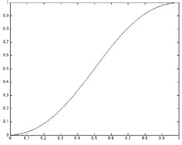
restricted function h(ξ). To create h(ξ), a smooth transition from 1 to 0, we begin

by integrating bump functions.

Integrating Bump Functions for Smooth Transitions

We arrive ath(ξ) by integrating smooth bump functions,g(y) with suppg ⊂[0, τ]

and then flipping them. Specifically,

h∗(ξ) = Rτ 1

0 g(y) dy

Z ξ

0

g(y) dy

and

h(ξ) =h∗(τ −ξ) = _Rτ 1

0 g(y) dy

Z τ−ξ

0

Figure 2.1 A Smooth Transition from 0 to 1 with τ = 1

This creates our smooth transition from 1 to 0. We then attach this on both sides

of our block of values 1 on [−1,1] to extend the support to [−1−τ,1 +τ] and arrive

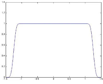
at our ϕ(ξ) that satisfies our algorithm all the way up to approximating f at anyx.

Finally we arrive at

ϕ(ξ) :=



             

             

h∗(ξ+ 1 +τ) x∈[−1−τ,−1)

1 x∈[−1,1]

h(ξ−1) x∈(1,1 +τ]

Figure 2.2 Example of ϕ with τ = 1 2

Thus we have ϕdefined and therefore,

KN = 1 + 2

M

X

j=1

ϕ j N

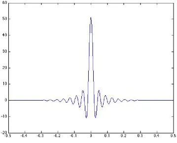
Figure 2.3 Example of K30 with τ = 1₂

We now work our way back up in the next section, implementation.

2.2 Implementation

Example Bump Functions

We begin our implementation of the algorithm by a few choices of g(y), the bump

g1(y) = (y(τ −y))b

g2(y) =

sinyπ

τ b

g3(y) =e −1 y(τ−y)

g4(y) =eb √

y(τ−y)

for some b’s.

Example Smooth Transitions

We then calculate the respective h∗’s andh’s:

h∗₁(ξ) = Rτ 1

0 (y(τ −y))b dy

Z ξ

0

(y(τ −y))b dy

h∗₂(ξ) = Rτ 1

0 (sin yπ τ ) b _dy Z ξ 0 (sin yπ τ ) b _dy

h∗₃(ξ) = 1

Rτ

0 e −1 y(τ−y) _dy

Z ξ

0

e

−1 y(τ−y) _dy

h∗₄(ξ) = 1

Rτ

0 e

b√y(τ−y) _dy

Z ξ

0

eb

√ y(τ−y)

dy

and

h1(ξ) =

1

Rτ

0 (y(τ−y))b dy

Z τ−ξ

0

(y(τ−y))b dy

h2(ξ) =

1

Rτ

0 (sin yπ

τ )b dy

Z τ−ξ

0

(sinyπ

τ )

b _dy

h3(ξ) =

1

Rτ 0 e

−1 y(τ−y) dy

Z τ−ξ

0

ey(−τ−1y) _dy

h4(ξ) =

1

Rτ

0 e

b√y(τ−y) _dy

Z τ−ξ

0

eb

√

y(τ−y) _dy.

Note that h4(ξ) does not necessarily end at 0. This means it is not an ideal

transition. However, it still serves as a valid function since we may assume the next

sample to take value 0, and any continuous function with compact support can be

Trapezoidal Quadrature Formula

We begin by letting ˜M ∈_Nbe large. Then for tk := _Mk˜τ, we approximate by,

Z tk

0

h(x)dx≈ τ

˜

M

k

X

j=0

h(tj)−

1

2h(0)− 1 2h(tk)

.

Approximating the Smooth Transition

The first step in is evaluating the smooth transitions. To this end, we either

calculate the integral directly (in the case ofh1(ξ)) or use a quadrature formula. For

instance, the trapezoidal with a high number of sample points, ˜M, from above.

From here we calculateh(_Nj ) forj = 0,1,2, . . .bτ Nc; these are equispaced samples.

We attach these onto an array of size N where the values are all 1. This makes an

array of samples of the positive side of ϕ. Since ϕis symmetric this is all we need.

With ϕ in hand, we now compute the sampled points of KN(x). To do this we

either tack on an array of 0’s to ourϕarray and compute the inverse fourier transform

(preferably using the inverse fast fourier transform) or we compute the points directly

using the formula:

KN(x) = 1 + 2 M

X

j=1

ϕ j N

cos 2πjx.

We now have a large number of sampled points of KN(x) to work with, let this

number beW many points. KN(x) should be well localized thanks to our selection of

ϕ. Thus we may cut off the tails of KN(x). I.e., we restrict the support of KN(x) to

[−δ, δ] when

KN(x)

< ∀x∈[−

1

2,−δ)∪(δ, 1

2] for δ dependent on and is chosen

to meet our error requirement.

Approximation of the Kernel Using Lagrange Interpolation

From here we approximate KN(x) at any x using Lagrange Interpolation on the

remaining points. Let

KN

n W

a

n=−a

trun-cation. Then our approximating function of KN(x) using Lagrange Interpolation is

given by

f

KN(x) := a

X

j=−a

KN

j

W

Y

−a≤n≤a n6=j

x− n W j W −

n W

.

Finalizing the Kernel

Now that we have an approximate KN at any x, we may apply our original

quadrature formula for approximation off at any xusing only the sampled points of

f. Let xj = _M+Nj , then:

f(x)≈ 1

M +N

M+N−1

X

j=0

f

KN(x−xj) f(xj).

And since we have supp KN(x)⊂[−δ, δ], we further restrict this sum:

f(x)≈ 1

M +N

M+N−1

X

j=0 |x−xj|≤δ

f

Chapter 3

Nonequispaced Fast Fourier Transform:

Algorithm 2

In the chapter, we examine another algorithm for fast and accurate evaluation of

high degree trigonometric polynomials at many scattered points. This algorithm was

proposed by A. Dutt and V. Rokhlin in [?] and further developed by other authors,

see e.g. [?]. Our goal is to compare the performance of the algorithm of Dutt and

Rokhlin with the algorithm we developed in Chapter 2. For convenience we shall use

the notation from [?].

Similarly as before we are interested in the following

Problem. Given the Fourier coefficients {fˆk}

N 2−1

k=−N 2

, N even, compute the values of

the trigonometric polynomial

f(x) = N

2−1

X

k=−N 2

ˆ

fke−2πikx (3.1)

at many scattered points {xj}Mj=1.

3.1 The idea of the algorithm

Start by defining IN :={k :−N₂ ≤k < N₂}. Then f(x) =Pk∈IN ˆ

fke−2πikx. The idea

is to approximate f(x) using a linear combination of the shifts of very well localized

1-periodic function ˜ϕ, that is,

f(x)≈s1(x) :=

X

j∈In

gjϕ˜

x− j

n

, (3.2)

An important component of this method is to define the function ˜ϕ by

one-periodization of a very well localized smooth window functionϕ, i.e.

˜

ϕ(x) := X

r∈Z

ϕ(x+r) = X

r∈Z

ck( ˜ϕ)e−2πikx,

serving a similar role as ϕ in Chapter 2 and having a similar localization. We will

assume that ϕ is in the Schwartz class S(_R), i.e. ϕ ∈ C∞(_R) and for any k, ` ≥ 1

there exists a constant c(k, `) > 0 such that|ϕ(k)(x)| ≤ c(k, `)(1 +|x|)−` for x ∈ _R.

Above ck( ˜ϕ) is thekth Fourier coefficients of the 1-periodic function ˜ϕ. Thus

ck( ˜ϕ) =

Z

T

˜

ϕ(x)e2πikxdx=

Z 1

0

X

r∈Z

ϕ(x+r)

e2πikxdx.

We now interchange summation and integration and apply a change of variables

u=x+r after multiplying by e2πikr _{= 1 to obtain}

ck( ˜ϕ) =

X

r∈Z

Z 1

0

ϕ(x+r)e2πik(x+r)dx=X

r∈Z

Z r+1

r

ϕ(u)e2πikudu=

Z

R

ϕ(u)e2πikudu= ˆϕ(k).

Therefore,

s1(x) =

X

j∈In

gjϕ˜

x− j

n

= X

j∈In

gj

X

k∈_Z

ck( ˜ϕ)e−2πik(x−

j n)

=X

k∈_Z

X

j∈In

gje2πi

k nj

ck( ˜ϕ)e−2πikx.

We define

ˆ

gk:=

X

j∈In

gje2πi

k

nj, (3.3)

and note that {gˆk} is n-periodic. We split the above sum into two

s1(x) =

X

k∈Z

ˆ

gkck( ˜ϕ)e−2πikx =

X

k∈In ˆ

gkck( ˜ϕ)e−2πikx+

X

k∈_Z\In ˆ

gkck( ˜ϕ)e−2πikx,

where similarly as aboveIn:={k:−n₂ ≤k < n₂}. Using then-periodicity of {ˆgk}we

obtain

X

k∈_Z\In ˆ

gkck( ˜ϕ)e−2πikx =

X

r∈_Z\{0}

X

k∈In ˆ

gnr+kck+nr( ˜ϕ)e−2πi(k+nr)x

= X

r∈Z\{0}

X

k∈In ˆ

Hence

s1(x) =

X

k∈Z

ˆ

gkck( ˜ϕ)e−2πikx=

X

k∈In ˆ

gkck( ˜ϕ)e−2πikx+

X

r∈Z\{0}

X

k∈In ˆ

gkck+nr( ˜ϕ)e−2πi(k+nr)x.

As ϕ∈ S(_R) the coefficients ck( ˜ϕ) = ˆϕ(k) are small for |k| ≥n and hence

X

r∈Z\{0}

X

k∈In ˆ

gkck+nr( ˜ϕ)e−2πi(k+nr)x

≤ε

for some ”small” constant ε >0. Thus

s1(x)≈

X

k∈In ˆ

gkck( ˜ϕ)e−2πikx.

We also assume that ck( ˜ϕ) 6= 0 for k ∈ IN. Now, comparing the above with (??)

suggests to set ˆfk = ˆgkck( ˜ϕ). More precisely, we set

ˆ

gk :=

         ˆ fk

ck( ˜ϕ) for k ∈IN,

0 for k ∈In\IN.

Then the values{gj} can be obtained from (??) by

gj =

1

n X

k∈IN ˆ

gke−2πi

k nj

applying FFT of sizen, see §??.

The next step is truncate the “long“ sum in (??). The good localization of ϕ(x)

motivates its approximation by

ψ(x) =ϕ(x)1[−m_n,m_n](x),

where1_[−m n ,

m

n](x) is the characteristic function of [−

m n,

m n], and

m

n

1

2. The 1-periodic

version ˜ψ of ψ is defined by

˜

ψ(x) = X

r∈Z

ψ(x+r)

and we observe that

˜

ψ(x) =ψ(x) = ϕ(x)1[−m n,

m

Thus we arrive at the following approximation

f(x)≈s1(x)≈s(x) =

X

j∈In,m(x)

gjψ˜

x− j

n

= X

j∈In,m(x)

gjϕ

x− j

n

, (3.4)

where

In,m(x) :=

k ∈In:

x− k n ≤ m n

={k∈In:nx−m≤k ≤nx+m}.

One uses the “short“ sum on the right in (??) to approximate f(x) at arbitrary

scattered points {xj}mj=1.

3.2 Description of the algorithm

Here we describe the algorithm for evaluation of f(x) from (??) and arbitrary

scat-tered points {xj}Mj=1 ⊂R.

Input: N, M ∈_N, {fˆk}k∈IN ⊂C, {xj}

M

j=1 ⊂R.

One first precomputes the coefficients ck( ˜ϕ) = ˆϕ(k) fork ∈IN and then proceeds

as follows:

(1) For k ∈IN compute

ˆ

gk=

ˆ

fk

ck( ˜ϕ)

= ˆ

fk

ˆ

ϕ(k).

(2) For j ∈In compute by FFT

gj =

1

n X

k∈IN ˆ

gke−2πi

k nj.

(3) For j = 1,2, . . . , M compute

fj =

X

j∈In,m(xj)

gjϕ

xj−

j n

.

Output: Approximate values {fj}Mj=1.

Remark. The above algorithm requires the development of an algorithm and code

for fast and accurate evaluation ofϕ(x) at an arbitrary pointx∈h−m

n, m

n

i

and ˆϕ(k)

3.3 Window functions and error bound

Several window functions with good localization in space and frequency domain have

been proposed:

(a) The Gaussian

ϕ(x) = (πb)−1/2e−(nxb)2

b:= 2σm

π(2σ−1)

,

ˆ

ϕ(k) = 1

ne

−bπk_{n .}

(b) B-splines

ϕ(x) = M2m(nx),

ˆ

ϕ(k) = 1

nsinc

2m_(πk/n),

whereM2mis the centered cardinal B-spline, i.e. M2m(x) :=1[−1,1]∗1[−1,1]∗· · ·∗1[−1,1]

with the convolution applied 2m times and sinc ξ = sin_ξξ.

(c) Sinc function

ϕ(x) = N(2σ−1)

2m sinc

2mπnx(2σ−1)

2m

,

ˆ

ϕ(k) = M2m

_2mk

(2σ−1)N

.

(d) Kaiser-Bessel functions

ϕ(x) = 1

π            sinh

b√m2_−n2_x2

√

m2_−n2_x2 for |x| ≤

m

n, (b:=π(2−1/σ)),

sin

b√m2_−n2_x2

√

m2_−n2_x2 for |x|>

m n,

ˆ

ϕ(k) = 1

n          I0

mqb2_−(2πk/n)2 _{for −n1−} 1 2σ

≤k ≤n1− 1 2σ

,

0 otherwise ,

where I0 is the modified zero-order Bessel function.

The following error estimate has been proved in [?] in the case (a) of the Gaussian:

|f(xj)−fj| ≤4e−πm(1−1/(2σ−1))

X

k∈IN

|fˆ(k)|.

Similar error estimates are established in cases (b) - (d), see [?]. The above

esti-mate shows the Nonequispaced Fast Fourier Transform presented above is a viable

algorithm for evaluation of high degree trigonometric polynomials.

3.4 Complexity

As was shown in §?? the Fast Fourier Transform requires O(nlogn) operations.

On the other hand, the parametermis a “small“ constant. Therefore, the complexity

of the above described algorithm is O(NlogN+M).

It should be pointed out that the direct computation of the values f(xj), j =

1,2, . . . , M, of the trigonometric polynomial from (??) requires O(M N) operations,

Bibliography

[1] J. Berrut, L. Trefethen, Barycentric Lagrange Interpolation, SIAM Review, 46

(2004), 500-517.

[2] A. Dutt, V. Rokhlin, Fast Fourier transforms for nonequispaced data, SIAM J.

Sci. Stat. Comput. 14 (1993), 1368–1393.

[3] B. Elbel, G. Steidl, Fast Fourier transform for nonequispaced data, In C. K.

Chui and L. L. Schumaker, editors, Approximation Theory IX, Nashville, 1998, Vanderbilt University Press.

[4] L. Grafakos,Classical Fourier Analysis, Springer, New York, 2008.

[5] K. Ivanov, P. Petrushev, Fast memory efficient evaluation of spherical

polyno-mials at scattered points, Adv. Comput. Math. 41 (2015), no. 1, 191–230.

[6] K. Ivanov, P. Petrushev, Highly effective stable evaluation of bandlimited

func-tions on the sphere, Numer. Algorithms, 71 (2016), no. 3, 585–611.

[7] J. Keiner, S. Kunis, D. Potts, Using NFFT 3–a software library for various

nonequispaced fast Fourier transforms, ACM Trans. Math. Software 36 (2009), no. 4, 19:1–19:30.

[8] E. Stein, G. Weiss, Fourier analysis on Euclidean spaces, Princeton University

Appendix A

Code

Here we include some MATLAB code for the method discussed in Chapter 2.

Using this code to test the four Kernels with a exponent (where applicable) of 7, aτ

of 1, oversampling 30 times, a cut-off of 10−9_{(decimation of the Kernel), and with f of}

degree 50: the Square Root Exponential (h4) had an average error of 5.3×10−13, the

Gaussian (h3) had an average error of 9.0×10−11, the Power Sine (h2) had an average

error of 1.3×10−10_{, and the Polynomial (h}

1) had an average error of 1.7×10−10.

These values were found after computing 1000 random points per randomly generated

f, 200 times.

A.1 Algorithm 1

1 f u n c t i o n [ out ] = A l g o r i t h m 1 ( in , h a t f , tau , e p s i l o n ,

oversamp , p , b )

2 %APPROX1 R e a l i z a t i o n o f A l g o r i t h m 1

3 % i n : p o i n t s o f a p p r o x i m a t i o n

4 % h a t f : f o u r i e r c o e f f i c i e n t s o f t h e approximated

f u n c t i o n

5 % tau : c h o i c e o f tau ( l e n g t h o f e x t e n s i o n i n f o u r i e r

domain )

6 % e p s i l o n : c u t o f f a m p l i t u d e f o r t h e k e r n e l

8 % p : c h o i c e o f p h i ( 1 SqrtExpo , 2 Expo , 3 S i n e , 4

Poly )

9 % b : f o r p h i where t h e r e i s a s e l e c t a b l e b

10

11 MN = f l o o r((2+ tau )∗s i z e( h a t f , 2 ) ) ;

12 n od e s = 0 : 1 /MN: (MN−1)/MN;

13

14 %These a r e t h e sampled p o i n t s o f f

15 %Can u s e FFT h e r e o r a l r e a d y have t h e s a m p l e s precomputed /

sampled

16 f = D i r e c t E v a l ( nodes , h a t f ) ;

17

18 s w i t c h p

19 c a s e 2

20 p h i = E x p o F o u r i e r K e r n e l ((1+ tau )∗s i z e( h a t f , 2 ) , tau ) ;

21 c a s e 3

22 p h i = S i n e F o u r i e r K e r n e l ((1+ tau )∗s i z e( h a t f , 2 ) , b , tau ) ;

23 c a s e 4

24 p h i = P o l y F o u r i e r K e r n e l ((1+ tau )∗s i z e( h a t f , 2 ) , b , tau ) ;

25 o t h e r w i s e

26 p h i = S q r t E x p o F o u r i e r K e r n e l ((1+ tau )∗s i z e( h a t f , 2 ) , b ,

tau ) ;

27 end

28

29 %s e t t i n g up f o r t h e o v e r s a m p l e d k e r n e l

30 s n o d e s = 0 : 1 / ( oversamp∗MN) : ( oversamp∗MN− 1 ) / ( oversamp∗MN) ;

32

33 %c a l c u l a t i o n o f t h e o v e r s a m p l e d k e r n e l

34 f o r j = 1 : oversamp∗MN,

35

36 temp = 0 ;

37

38 f o r k = 1 :s i z e( phi , 2 ) ,

39

40 temp = temp + p h i ( k )∗c o s( 2∗p i∗k∗s n o d e s ( j ) ) ;

41

42 end

43

44 K( j ) = 1 + 2∗temp ;

45

46 end

47

48 %D e c i m a t i o n o f K when s t r i c t l y under e p s i l o n ( from t h e t a i l s )

49 f o r i = 1 :f l o o r(s i z e(K, 2 ) / 2 ) ,

50 i f abs(K(f l o o r(s i z e(K, 2 ) / 2 )−i +1) ) > e p s i l o n . . .

51 | | abs(K(f l o o r(s i z e(K, 2 ) / 2 )+i−1) ) > e p s i l o n ,

52 b r e a k;

53 end

54 K(f l o o r(s i z e(K, 2 ) / 2 )−i +1) = 0 ;

55 K(f l o o r(s i z e(K, 2 ) / 2 )+i−1) = 0 ;

56 end

57

59 out = i n∗0 ;

60

61 f o r i = 1 :s i z e( out , 2 ) ,

62

63 tempK = n od e s∗0 ;

64

65 f o r j = 1 :MN,

66

67 tempK ( j ) = Lagrange ( n o de s ( j )−i n ( i ) ,K, 4 ) ;

68

69 end

70

71 f o r j = 1 :MN,

72

73 out ( i ) = out ( i ) + tempK ( j )∗f ( j ) ;

74

75 end

76

77 end

78

79 out = out /MN;

80