ESTIMATION OF QUASI-STATIC
J
-
R
CURVES FROM CHARPY
ENERGY AND ADAPTATION TO ASTM E 1921 REFERENCE
TEMPERATURE ESTIMATION OF FERRITIC STEELS
P.R. Sreenivasan1
1Metallurgy and Materials Group, Indira Gandhi Centre for Atomic Research, Kalpakkam, Tamilnadu,
INDIA-603102
E-mail of corresponding author: [email protected]
ABSTRACT
Many researchers had suggested a sort of scaling procedure for predicting the quasi-staticJ-Rcurves from dynamic
J-Rcurves obtained from instrumented Charpy V-notch (CVN) impact tests using key-curve, compliance or other procedures. Chaouadi, based on extensive tests and literature data, had quantitatively formalized the method and suggested general applicability of his method for a class of steels. In this paper, first, Chauoadi-procedure is tried on some selected data from the literature (including the data used by Chaouadi and other workers) and an adaptation of the method is suggested using Wallin’s as well as Landes’s lower bound methods for upper-shelf J-R curve estimation from CVN energy. Using Chaouadi and other data as the benchmark, suitable scaling factors have been determined that enable estimation of quasi-staticJ-Rcurves from CVN energy alone, without the need for dynamic CVNJ-Rcurves. The final formulae are given. This new method can be called modified Wallin-Landes procedure. Then this method is applied to fracture toughness and reference temperature (T0– ASTM E-1921) estimation from
the full Charpy-transition data. The results are compared with those from the author’s IGC-procedure, and modifications , if any, are suggested. Based on the new results, it is suggested that the IGC-procedure may be modified as: finalTQ-est=TQ-IGC for TQ-Schdy ≤ 20 °C (in the IGC-procedure the dividing temperature was 60 °C);
and forTQ-Schdy> 20 °C, TQ-IGC=TQ-WLm(different from the IGC-procedre and subscript WLm indicating modified
Wallin-Landes procedure). For the 59 or more steels examined (including highly irradiated steels), the TQ-WL
estimates at higher temperatures are consistent and conservative; a few non-conservative values are acceptably less than 20 °C, where as other predictions show non-conservatism of up to 40-50 °C. At lower temperatures,TQ-IGC is
consistently conservative and not over-conservative as the other estimates. The limitations suggested by Chaouadi for his method, namely, dependence on work-hardening, strain rate, yield stress, etc., hold good for the present method also and require further quantification based on finite element analysis, if necessary; however, these are not likely to affect theTQestimation significantly. KJ-WLmis better than RNB correlation in making a conservative or
closer estimate of fracture toughness at the upper shelf.
INTRODUCTION
Charpy V-notch impact (CVN) test is very attractive because of its low-cost, simplicity and wide familiarity and availability compared to the more sophisticated and costly fracture mechanics test which requires very skilled manpower and special instumentation [1,2]. For quantitative design involving assurance of structural integrity, fracture toughness data in terms ofKIC,JICor, its engineering equivalent,J0.2, and fracture resistanceJ-R
curves are required. To achieve this, many Charpy-fracture toughness correlations have been proposed; because of differences in loading rate, notch acuity, constraint etc. between the Charpy and fracture toughness tests, these lack universal applicability and are restricted to the specific material and test conditions for which they were derived [1-9]. However, some of the recent correlations are more promising from the point of view of producing design relevant fracture toughness properties that are consistently, and, often, assuredly, conservative [1,9]. This paper is an attempt to further extend these efforts. Aurich et al. [4] and Tronskar et al. [5] had suggested a sort of scaling procedure for predicting the quasi-static J-R curves from dynamic J-R curves obtained from instrumented CVN impact tests using key-curve, compliance or other procedures. They had given approximate scaling factors. Chaouadi [1,6], based on extensive tests and literature data, had quantitatively formalized the method and suggested general applicability of his method for a class of steels. Chaouadi [1] had suggested the need for quantifying the variation of the scaling factors depending on work-hardening index, yield stress, strain rate etc., based on finite element analysis also. In this paper, using Chaouadi and other data as the benchmark, an adaptation of the method is suggested using Wallin’s [7] as well as Landes’ [8] methods for upper-shelfJ-Rcurve estimation from CVN energy. Methodolgy for obtaining the suitable scaling factors has been oulined that will enable estimation of quasi-staticJ-R
results discussed. This new method can be called modified Wallin-Landes procedure. Then this method is applied to fracture toughness and reference temperature (T0– ASTM E-1921 [10]) estimation from the full Charpy-transition data. The results are compared with those from Sreenivasan's [9] IGC-procedure and modifications, if any, are suggested. Also, the effectiveness of the new formulae in predicting the upper-shelf fracture toughness is examined and compared with the results from the well known Rolfe-Novak-Barsom (RNB) equation [3].
BASIC METHODOLOGY AND MATERIALS Basic Methodology
Fig. 1. Illustration of the Wallin and Landes procedure predictions and derivation of scaling factors
a/ mm
0.0 0.2 0.4 0.6 0.8 1.0 1.2 1.4 1.6
J
/
k
J
.m
-2
0 200 400 600 800 1000 1200
0 200 400 600 800 1000 1200 QSJR- CT25 test
JW
JL
JWLm
JCh
JR CVN dynamic
Steel: E460(3) tested at 200C
ys= 480 MPa;yd= 626 MPa
Charpy energy,CV= 104 J
AverageJR-QS/JW: 1.55
AverageJR-QS/JL: 2.295
Aurich et al. [4] and Tronskar et al. [5] had suggested the possibility of obtaining quasi-staticJ-Rcurves from dynamicJ-Rcurves obtained from instrumented impact tests of blunt-notched or precracked CVN specimens using appropriate scaling. The scaling factor was determined empirically, often with an additional factor involving the ratio of dynamic to static yield stress. Chaouadi and Puzzolante [1,6] had formalised these efforts in the following equations:
2 yd
static CVN impact
LR config ys
.
.
.
(1)
R R
J
J
which for dynamicJRreduces to:CVN impact
config
.
(2)
dynamic
R R
J
J
where,JRCVN impact, represents the dynamicJR-curve obtained from CVN impact test using key-curve, compliance or
other procedures [1,6,11] andJRdynamicandJRstaticare the dynamic and quasi-staticJR-curves, respectively, obtained
from deeply precracked specimens using standard fracture toughness tests; αLR is a loading rate factor, βconf is a
factor accounting for notch acuity and configuration effects (V-notch vs. fatigue precrack),σydandσysare dynamic
and static yield stress, respectively, at the test temperature. The square term arises from the consideration thatJR(J
Chauoadi [1] has empirically determinedαLR= 0.46;βconfis given to be 0.52 at quasi-static loading rate and 0.84 at
impact loading rate. JRstaticobtained from Eq. (1) using Chaouadi’s factors (αLR = 0.46 andβconf = 0.52) may be
termedJCh. Figure 1 illustrates the application of Eq. (1) to the results for a C-Mn steel - E 460(3) – given in Aurich
et al. [4].
Now, one disadvantage of the above procedure is that it requires instrumented impact test facility and sophisticated and careful data processing to obtainJRCVN impact, that is, the dynamicJR-curve from CVN impact test. Recently, Wallin [7] as well as Gioielli, Landes et al. [8] have derived semi-empirical equations for estimating the static JR-curve from the CVN energy, CV (because of the unfamiliarity and difficulty of the name Gioielli, for
convenience, the procedure or equation due to the latter is referred as Landes’ equation in this paper; Prof. Landes is well known in the elastic-plastic fracture field). Wallin’s [7] near-lower-bound correlation for predominantly ductile fracture (especially applicable to Charpy upper-shelf – US - region) is applicable in the temeperature region -100 to 300 °C. In fact, this new correlation gives not only the initiationJ-value, but also theJ-Δatearing resistance curve (J-Rcurve) as a function ofCVvalues in the US. The correlations are as given below:
m -2
W 1mm
[kJ.m , mm]
(3)
J
J
a
where
1.28 -2
1mm V-US
20
= 0.53
exp(
) [kJ.m , J, C]
(3a)
400
T
J
C
and
ys-RT 0.256
V-US
20
= 0.133
exp(
)
+ 0.03 [J, C, MPa]
(3b)
2000
4664
T
m
C
where σys-RTis the yield stress at room temperature,CV-USis the upper-shelfCVvalue andTis the test temperature.
The equation due to Landes [8] is as given below:
0.5 2
V-US
L = 139.75 ( ) [kJ.m ,J, m] (4)
3.15 C
J a
TheJvalue from Eq. (3), that is due to Wallin, will be referred asJW, and that from Eq. (4), that is due to Landes,
will be referred asJL. TheJWandJLobtained for the steel in Fig. 1 are shown along with the quasi-staticJR-curve
(QS-JRorJR-QS).
As Eqs. (3) and (4) already incorporate a sort of notch effect and strain rate factors, only a simple multiplicative scaling is considered sufficient (unlike in the case of Eqs. (1) and (2)). The scaling factors are obtained by taking the ratios ofJR-QS/JWandJR-QS/JL; the average ratios obtained for the results in Fig. 1 are 1.55 and 2.295, respectively (i.e., over the whole range of Δa= 1.4-1.5 mm shown in Fig. 1). Similarly, ratios are found for various other steels. Other results and comparisons are given in detail later.
Materials
For calibration of the procedure, that is for determining the scaling factors as discussed in the previous paragraph, the data for the steels tested mainly at 20-25ºC or 280-300ºC and described in Aurich [4], Blauel [12], Eberle [13], Yoon [14] and El-Fadaly [15] have been used. For later comparison of the reference temperature estimates, apart from the above steels (only those for which full transition range Charpy data are available), all the steels described in Sreenivasan [9] have been used along with a few other steel data culled from recent literature, which are not listed here to restrict the bulk of the paper.
RESULTS AND DISCUSSION
Modified Wallin-Landes Procedure forJRcurve estimation
For calibration, the scaling factors,JR-QS/JWandJR-QS/JL, have been determined for the steels listed in Table
1. The average scaling factors are 1.656 and 2.146 forJR-QS/JWandJR-QS/JL, respectively, though for the particular
steel shown in Fig. 1, they were 1.55 and 2.295, respectively. For the present purpose, for representing the material
and (4) respectively. The JR-curve based on the mean value is called the J based on modified Wallin-Landes
procedure, represented byJWLm(subscript indicating Wallin-Landes-modified). This is given as Eq. (5).
a/ mm
0.0 0.5 1.0 1.5 2.0
J
/
k
J
.m
-2
0 200 400 600 800 1000 1200
JRCVN dynamic- X-52 steel
QS-JR- X-52 steel
JCh- X-52 steel
JWLm- X-52 steel
JRCVN dynamic
- CrMoNi steel
JCh- CrMoNi steel QS-JR- CrMoNi steel
JWLm- CrMoNi steel
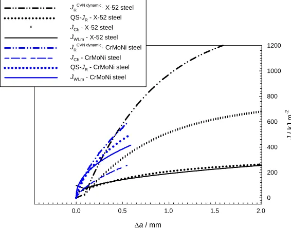
Fig. 2. Application of the modified Wallin-Landes procedure to an X-52 grade pipeline steel (Tyson et al. [16]) and a CrMoNi steel (Blumenauer et al. [17])
Table 1. Scaling factors determined for various steels (source references listed in square brackets)
Steel
JR-QS/JR-W JR-QS/JR-L
Test Temp/ ºC
CV/ J YS/MPa
Eberle:St460 [13] 1.8420 2.5130 25 78 470
Aurich:E460(3) [4] 1.5500 2.2950 20 104 480
Blauel :20MnMoNi55[12] 1.3880 1.8790 80 161 464
Blauel:20MnMoNi55 [12] 1.3947 1.5992 150 155 441
Blauel:20MnMoNi55 [12] 2.1073 1.6550 300 145 433
20MnMoNi55:BM [15] 1.6460 2.8230 25 194 454
20MnMoNi55: -10%PD [15] 1.1390 1.9360 25 201 509
Yoon:Mod9Cr1Mo [14] 1.7640 2.8340 25 187 520
Yoon:Mod9Cr1Mo [14] 2.0732 1.7750 288 260 476
Computed values
Mean 1.656 2.146
SD 0.325 0.485
Std. Error 0.108 0.162
95% Confidence Level 0.250 0.373 99% Confidence Level 0.363 0.543
W L
WLm
1.656 2.146
= (5)
2
J J
J
In Fig. 1, theJWLmcurve shows fair agreement with theJR-QScurve; in fact, it shows much better agreement with the JR-QScurve than the curve obtained by the Chaouadi procedure,JCh(Eq. (1)). For all the steels for which
compared with the respective quasi-staticJR curves (all the data used in the present calibration are different from
those used by Chaouadi). Hence, this agreement is very satisfactory.
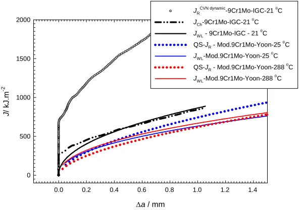
Fig. 3. Comparison of theJWLmwithJChorJQS(QS-JR) for a 9Cr1Mo steel [18] and a modified 9Cr1Mo steel [14]
a/ mm
0.0 0.2 0.4 0.6 0.8 1.0 1.2 1.4
J
/
k
J
.m
-2
0 500 1000 1500 2000
JR
CVN dynamic-9Cr1Mo-IGC-21C
JCh-9Cr1Mo-IGC-21
C
JWL- 9Cr1Mo-IGC - 21
C
QS-JR- Mod.9Cr1Mo-Yoon-25
C
JWL-Mod.9Cr1Mo-Yoon-25C QS-JR- Mod.9Cr1Mo-Yoon-288
C
JWL-Mod.9Cr1Mo-Yoon-288
C
In fact, for some different steels, for which the Chaouadi method doesn’t work, use of Eq. (5) results in excellent agreement with the QS data. Two such cases are shown in Fig. 2. For the X-52 steel the agreement extends to very large crack extension upto 6-7 mm while for the CrMoNi steel, the theJWLmcurve is acceptably conservative
at large crack extensions. The results for a 9Cr1Mo steel [18] and a modified 9Cr1Mo steel [14] are presented in Fig. 3. The dynamicJR curve for the 9Cr1Mo steel shown in Fig. 3 was determined by Sreenivasan [18] from the
instrumented impact test results of CVN (non-precracked) specimens by applying the key-curve procedure described in Sreenivasan et al. [11]; the agreement between theJChandJWLmcurves is quite good. For the modified 9Cr1Mo
steel (Yoon et al. [14]) shown in Fig. 3, the 25 °C results are acceptably (but not excessively) conservative (i. e.,
JWLm<JQS) while the 288 °C results are non-conservative, but within the scatter expected forJvalues - Sreenivasan
et al. [19]. The relevant mechanical data for the steels shown in Figs. 2 and 3 are given in Table 2.
Table. 2. Relevant mechanical data for steels shown in Figs. 2 and 3 (source references listed in square brackets)
Steel Test Temp/
°C
YS / MPa
Dy. YS / MPa
CV/ J RT-YS /
MPa
Remarks
X-52 (Tyson et al. [16]) 23 376 554 65.5 376 IIT*+ QS#
CrMoNi (Blumenauer et al. [17]) 25 447 603 160 447 IIT+ QS
9Cr1Mo (Sreenivasan [18]} 21 515 668 244 515 Only IIT
Mod. 9Cr1Mo (Yoon et al. [14]) 25 525 670 187 525 No IIT
Mod. 9Cr1Mo (Yoon et al. [14]) 288 476 473 260 525 No IIT
*: IIT - Instrumented Impact Test; #: QS – Quasi Static
Application ofKJ-WLmfor Estimation of ASTM E 1921 Reference Temperature (T0)
Modified Wallin-Landes procedure for JR curve estimation was described in the previous section. One
thing that emerges from the previous section is that though JR curve by the Wallin-Landes procedure may differ
from the actual QS-JRcurve (conservatively, and, sometimes, non-conservatively), the commonly used engineering
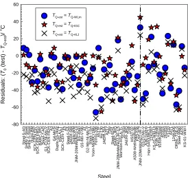
Fig. 4. Residuals various reference temperature estimates compared with that ofTQ-WL
Steel S te e l-5 -A D S H IN -T -S te e l S H IN -S -S te e l D u p lx -B M S C K -C E N E 9 7 S C K -C E N E M 1 0 B A R C -J P G S te e l-7 -A D G 1 -C r-N i-M o -V S C K -C E N F 8 2
H A3
G 4 -M n S i D u p lx -S S -H o lz H S L A -L T S C K -C E N -T 9 1 A 2 S te e l-5 -S A J A E R I-S tB D u p lx -W M J N M -2 0 M n M o N i2 2 -U I B S -4 3 6 0 G 5 -M n -V -N b A 1 G 2 -M n -N i-M o -V S te e l-7 -S A Y o o n -M o d 9 C r1 M o F e rr n o -3 3 6 A 5 1 7 F H y -1 3 0 J A E R I-S tA A 2 1 7 7 3 W S te e l-9 2 4 1 B A R C -J R Q J N M -2 0 M n M o N i2 2 -I R -3 .5 M o rr is o n -H S L A -T L 3 1 7 8 S t J A E R I-J R Q 7 2 W H S S T -0 2 A 5 0 8 -W e llm a n R o lf e F Z D -5 3 6 J N M -2 0 M n M o N i2 2 -I R -7 G 3 -C r-M o -V A 3 6 -S o re m H a n -S A 5 3 3 B C L 1 1 2 4 J 3 5 7 K S -0 1 -W ld -U I E U R -2 3 5 9 8 9 1 6 3 8 1 S te e l 4 0 3 S S 2 6 1 8 S t V 1 2 3 3 A 4 7 1 1 2 4 K 4 0 6 O R N L -T S E -5 S te e l-9 9 8 0 A 4 7 0 K S -0 1 -W ld -I R e s id u a ls : ( T0 (t e s t) -TQ -e s t )/ 0 C -80 -60 -40 -20 0 20 40 60
TQ-est=TQ-WLm
TQ-est=TQ-IGC
TQ-est=TQ-41J
correspondingKJ-WLm can be estimated by the usual conversion formula (KJ = √EJ/(1 - ν2)). Though Eqs. (3)-(5)
have been resticted to be applicable to the fully ductile upper shelf, for our purpose we remove that restriction and apply the Eqs. (3)-(5) over the whole range of Charpy transition to obtain the correspondingKJ, taking ∆a = 0.2 mm.
Then theKJ-WLmvalues corresponding to the straight line portion of the CVN transition curve are taken to estimate
an equivalent of T0. This can be done by superimposing an eye-fit straight on the linear portion of the Charpy
transition curve avoiding the lower shelf. Then starting from the lowest value on the straight line portion a range of
values up to 50-70 MPa√m above the lowest value are taken with the corresponding temperatures and these are
applied to the multi-temperature Wallin formula(Eq. (6)) to yield an estimate of T0, namely, TQ-WL. Since all the
calibrations given Table 1 pertain to 1" thick quasi-static test, theKJ-WLmvalues obtained fromJWLare considered as
pertaining to 1" specimen tests. Equation (6) is as given below [10,9]:
4
0 min 0
5
1 min 0 1 min 0
exp{0.019(
)
(
) exp{0.019(
)}
0
(6)
[31
77 exp{0.019(
)}]
[31
77 exp{0.019(
)}]
i n n
i i J WL i
i i i i
T
T
K
K
T
T
K
T
T
K
T
T
where the Kroneckeri= 1,Kmin= 20 MPam,Tiis the test temperature andT0=TQ-WL. The validity conditions and
other requirements as required by ASTM E 1921 [10] are not examined. TheKJ-WLmvalues for application in Eq. (6) range from 100-170 to 200-270 MPa√m, depending on the steel.
Figure 4 shows the residuals of the TQ-WL values (i. e., T0 (test) - TQ-WL) for about 59 steels (all steels mentioned in [9] plus some additional steels) in comparison with other estimates discussed in [9] (TQ-IGC:TQ-estbased
on the IGC procedure described by Sreenivasan [9] and TQ-41J: taking TQ-est = T41J, the 41J Charpy transition
temperature, a very conservative estimate). It can be seen thatTQ-WLis either as much conservative or more over the
whole range ofT0values ranging from about -140 to +140 °C examined in Fig. 4. The steels in Fig. 4 are arranged
with increasing TQ-Sch dy
(a dynamic fracture toughness based reference temperature estimate as described in [9] which is necessary to estimate TQ-IGC) from left to right ranging from -100 to 230 °C. In fact, for the high
temperature steels to the right of the vertical line shown in Fig. 4 (i. e., TQ-Schdy > ~20 °C), TQ-WLshows more
consistency in producing assuredly conservative values thanTQ-IGC. So the criterion given in [9] may be modified as: TQ-est=TQ-IGCforTQ-Sch
dy ≤ 20 °C and
TQ-est=TQ-WLforTQ-Sch dy
his method, namely, dependence on work-hardening, strain rate, yield stress, etc., hold good for the present method also and require further quantification based on finite element analysis, if necessary; however, these are not likely to affect theTQestimation significantly.
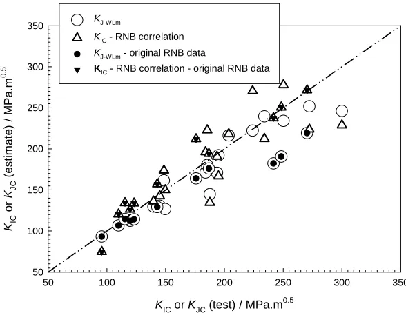
Fig. 5. Comparison ofKJ-WLm(fora= 0.2 mm) at the upper shelf with the predictions from RNB correlation for 27 steels
KICorKJC(test) / MPa.m0.5
50 100 150 200 250 300 350
KIC
o
r
KJ
C
(e
s
ti
m
a
te
)
/
M
P
a
.m
0
.5
50 100 150 200 250 300
350 KJ-WLm
KIC- RNB correlation
KJ-WLm- original RNB data
KIC- RNB correlation - original RNB data
KJ-WLm as an Upper Shelf Fracture Toughness Estimator
As described in the previous section, estimates ofJWLm values at the upper shelf corresponding to ∆a= 0.2
mm will give the upper shelfKJ-WLmusing the usual conversion formula. The results for 27 steels are shown in Fig. 5
in comparison with predictions from the RNB correlation [3]. The conservatism of the KJ-WLmfor all the steels is
obvious - closer to or below the 1:1 line. In fact, the filled symbols shown in Fig. 5 pertain to the 11 steels that went into the original RNB correlation.KJ-WLmis better than RNB correlation in making a conservative or closer estimate
of fracture toughness at the upper shelf.
CONCLUSION
Chaouadi procedure predicts the quasi-static J-R curves from dynamic J-R curves obtained from instrumented Charpy V-notch (CVN) impact tests. Wallin and Landes formulae predict lower bound upper shelf fracture toughness and quasi-staticJ-Rcurves from CVN energy. Using Chaouadi and other data as the benchmark, suitable scaling factors have been determined that enable estimation of quasi-static J-R curves from CVN energy alone by application of the Wallin and Landes formulae, without the need for dynamic CVNJ-Rcurves. The final formulae are given. This new method can be called modified Wallin-Landes procedure. Then this method is applied to fracture toughness and reference temperature (T0 – ASTM E-1921) estimation from the full Charpy-transition
data. The results are compared with those from the author’s IGC-procedure, and modifications , if any, are suggested. Based on the new results, it is suggested that the IGC-procedure may be modified as: finalTQ-est=TQ-IGC
for TQ-Schdy ≤ 20 °C (in the IGC-procedure the dividing temperature was 60 °C); and for TQ-Schdy> 20 °C, TQ-IGC=
TQ-WLm(different from the IGC-procedre and subscript WLm indicating modified Wallin-Landes procedure). For the
59 or more steels examined (including highly irradiated steels), the TQ-WL estimates at higher temperatures are
consistent and conservative; a few non-conservative values are acceptably less than 20 °C, where as other predictions show non-conservatism of up to 40-50 °C. At lower temperatures, TQ-IGC is consistently conservative
further quantification based on finite element analysis, if necessary; however, these are not likely to affect the TQ
estimation significantly. KJ-WLm is better than RNB correlation in making a conservative or closer estimate of fracture toughness at the upper shelf.
REFERENCES
[1] R. Chaouadi and J.L Puzzolante. Procedure to Estimate the Crack Resistance Curve from the Instrumented Charpy V–Notched Impact Test. ICF-12, Toronto, Canada, 2009.
[2] Sreenivasan, P. R. Instrumented Impact Testing—Accuracy, Reliability, and Predictability of Data,Trans. Indian Inst. Met., Vol 49 (No. 5), Oct. 1996, pp. 677–696.
[3] Nevasmaa P and Wallin K. STRUCTURAL INTEGRITY ASSESSMENT PROCEDURES FOR EUROPEAN INDUSTRY SINTAP TASK 3 STATUS REVIEW REPORT: RELIABILITY BASED METHODS. REP. SINTAP VTT/4 (SINTAP-3-2-1997). VTT Manufacturing Technology, Espoo, Finland, March 1997.
[4] D. Aurich, R. Helms, H.-J. Kuhn, K. Wobst and J. Ziebs. Charpy upper shelf energy and crack resistance.
Nuclear Engineering and Design,87, 1985, pp.109-121.
[5] J.P. Tronskar, M.A. Mannan, M.O. Lai. Correlation between quasi-static and dynamic crack resistance curves.Engineering Fracture Mechanics,70, 2003, pp.1527–1542.
[6] Chaouadi, J.L. Puzzolante . Loading rate effect on ductile crack resistance of steels using precrackedCharpy specimens,Int J Pres. Ves. Piping85, 2008, pp.752–761.
[7] K. Wallin. Low cost J–R curve estimation based on CVN upper shelf energy,Fat Frac Eng Mat Struc.,24, 2001, pp.537–549.
[8] P.C. Gioielli, J.D. Landes, J.D. Paris, H. Tada, L. Loushin. Method for predicting J–R curves from Charpy impact energy, in: P.C. Paris, K.L. Jerina (Eds.)Fatigue and Fracture Mechanics: 30th Volume,ASTM STP 1360, 2000, pp. 61–68.
[9] Sreenivasan P R. Inverse of Wallin’s relation for the effect of strain rate on the ASTM E-1921 reference temperature and its application to reference temperature estimation from Charpy tests.Nucl. Engng. and Design,241, 2011, pp. 67-81.
[10] ASTM E1921-97. Standard test method for determination of reference temperature,T0, for ferritic steels in
the transition range.Annual Book of ASTM Standards,Vol. 03.01, 1998, pp.1060-1076. ASTM, Philadelphia, USA.
[11] P.R. Sreenivasan and S.L. Mannan. DynamicJ-Rcurves and tension-impact properties of AISI 308 stainless steel weld.Int. J. Fracture,101, 2000, pp. 229–249.
[12] J. G. Blauel, L. Hodulak, T. Hollstein & B. Voss. Material Characterization by J-R Curves of a 20MnMoNi55 Forging.Int. J. Pres. Ves. & Piping17(1984) 139-162.
[13] A. Eberle, D. Klingbeil, J. Schicker.The calculation of dynamicJR-curves from the finite element analysis of a Charpy test using a rate-dependent damage model.Nuclear Engineering and Design198 (2000) 75–87.
[14] Ji-Hyun Yoon, and Eui-Pak Yoon.Fracture Toughness and the Master Curve for Modified 9Cr-1Mo Steel.
METALS AND MATERIALS International,12(6), 2006, pp. 477-482.
[15] M.S. El-Fadaly, T.A. E1-Sarrage, A.M. Eleiche, W. Dahl. Fracture toughness of 20MnMoNi55 steel at different temperatures as affected by room-temperature pre-deformation.Journal of Materials Processing Technology,54,1995, pp.159-165.
[16] W. R. Tyson, S. Xu and R. Bouchard. Correlation between J and CVN in upper shelf. In: From Charpy to Present Impact Testing (Charpy Centenary Conference, Poitiers, France, 2-5 Oct. 2001). D. Francois and A. Pineau (eds.). ESIS Publication 30, ESIS-Elsevier, Oxford OX5 IGB, UK, 2002, pp. 325-332. [17] Horst Blumenauer, Elfrun Schick and Rainer Ortmann. Elastic-plastic fracture-mechanics
assessment of a CrMoNi pressure vessel steel,Nuclear Engineering and Design,130(1991)pp.289-295. [18] P. R. Sreenivasan. Unpublished results. MMG, IGCAR, Kalpakkam, India (2004).