ABSTRACT
RATZLAFF, CHELSEA ROBYN. Detector Response Function for a Germanium Strip Type Detector/Imager. (Under the direction of John Mattingly).
Coded aperture imagers using high purity germanium (HPGe) dual sided strip detectors are a
technology that has become increasingly popular in the past ten years. Pioneers in this field
include Klaus Ziock et al. who developed the initial design of this type of detector and
Fenimore and Cannon in the field of coded aperture imaging. Ethan Hull of the company
PHDS is responsible for the detector design found in this project. These technologies
combine superior spectral resolution with position resolution to produce spectroscopic
images of unknown radiation sources. This has potential impacts in many fields from
homeland security to medical imaging. This research expands on an interpolation method by
M. Guttormsen et al. to create a detector response function. The response function is
pre-calculated using Monte Carlo transport, and uses MATLAB and Python scripts that pull from
a log of gamma ray interactions generated with MCNPX-PoliMi for individual source
energies and radial distances. MCNPX-PoliMi, a Monte Carlo transport code, was used to
create a model of the dual sided, electrode strip, cylindrical HPGe detector located at Oak
Ridge National Laboratory and created by the company PHDS. The detector was shown to
be radially symmetric, therefore cutting down on computational time by replacing the two
dimensional (x,y) pixel coordinates with a single radial position on the detector. The
response function interpolation was validated by comparing the MCNPX-PoliMi direct
calculations with the interpolated detector response function for a single source energy. In
addition, a direct calculation of the Ba-133 gamma spectrum was also compared to the
pre-calculated interpolated detector response function. The interpolated spectrum maintained the
general features of the spectrum but did exhibit some error compared to the direct
calculation. The error appears in the re-binning of the interpolated spectrum and could be
Detector Response Function for a Germanium Strip Type Detector/Imager
by
Chelsea Robyn Ratzlaff
A thesis submitted to the Graduate Faculty of North Carolina State University
in partial fulfillment of the requirements for the degree of
Master of Science
Nuclear Engineering
Raleigh, North Carolina
2014
APPROVED BY:
____________________________ ___________________________ Robin Gardner David Lalush
BIOGRAPHY
Chelsea Robyn Ratzlaff was born in Tulsa, Oklahoma on April 29, 1989. She grew up in
Asheville, NC and received her B.S. in Nuclear Engineering in May, 2012 from North
ACKNOWLEDGMENTS
Most importantly, I would like to thank the NCSU Nuclear Engineering Department and
specifically Dr. John Mattingly for giving me this great opportunity. Special thanks to Oak
Ridge National Laboratory (ORNL) for supporting me during this research and especially
Matthew Blackston at ORNL. In addition, I would like to thank Dr. Tony Nettleton for his
continued support, Casper Holmgreen for his programming insight, and Wesley Holmes for
his help and moral support. And, of course, I would like to say thanks to my friends and
family for putting up with me during my long hours of stress and coursework. Especially
TABLE OF CONTENTS
LIST OF TABLES ...v
LIST OF FIGURES ... vi
Chapter 1: Introduction ...1
1.1 Background and Motivation ...1
1.2 Scope of Thesis ...2
Chapter 2: Germanium Detectors and Response Functions ...6
2.1 Germanium Detector Fundamentals ...6
2.2 Gamma Spectroscopy ...10
2.2.1 Spectral Features ...10
2.2.2 Energy Resolution ...16
2.3 Coded Aperture Imaging with HPGe Strip Detector ...19
2.4 Detector Dimensions and Setup ...24
2.5 Detector Response Functions ...26
Chapter 3: Procedures for Calculating the Detector Response Function ...29
3.1 MCNPX-PoliMi Simulations ...29
3.2 Creating Detector Image ...32
3.3 Determining Source Beam Radius ...34
3.4 Determining Energies to Run ...39
3.5 Creating Input Files and Running Script on 32 CPUs ...40
3.6 Proving Radial Symmetry of the Detector ...42
3.7 Interpolating Separate Features of the Spectrum ...48
3.8 Re-binning Interpolated Energy Bins to MCNP Energy Bins ...56
Chapter 4: Results ...57
4.1 Calculated Response Function ...57
4.2 Single Energy and Radial Position Interpolated Response Function ...62
4.3 Ba-133 Decay Spectrum Using Interpolation Method ...66
Chapter 5: Conclusions ...78
LIST OF TABLES
Table 2.1: Properties of Germanium as a Semiconductor ... 8
Table 3.1: Important Detector Dimensions in MCNPX-PoliMi ...29
Table 3.2: Count Error for Comparing X and Y Directions ...44
LIST OF FIGURES
Figure 2.1: Semi-Conductor Detector Mechanics ...7
Figure 2.2: Gamma-Ray Spectrum Features ...11
Figure 2.3: Klein-Nishina Kernel ...13
Figure 2.4: Compton Continuum Shape ...14
Figure 2.5: Energy Resolution ...16
Figure 2.6: Pinhole Camera Diagram ...19
Figure 2.7: A Uniformly Redundant Array Coded Aperture ...20
Figure 2.8: Steps Involved in Coded Aperture Imaging ...21
Figure 2.9: Side Measurement of HPGe Strip Detector ...22
Figure 2.10: Front View Measurements of Detector ...23
Figure 2.11: Detector Setup ...24
Figure 2.12: Detector Setup Cont’d. ...25
Figure 2.13: Germanium Detector Response Function Example ...28
Figure 3.1: Front (a) and Back (b) Detector Views ...30
Figure 3.2: Front (a) and Back (b) Tilted Detector Views ...30
Figure 3.3: Detector/Source Setup ... 31
Figure 3.4: MCNPX PoliMi Log File Coordinates & Energy Deposited ...33
Figure 3.5: HPGe Strip Detector Image Running 109 Particles ...34
Figure 3.6: Setup for Determining Beam Width ...35
Figure 3.7: Detector Face Beam Width Visualization ...36
Figure 3.8: Center Pixel Counts vs. Source Beam Width ...37
Figure 3.9: Far Left Pixel Subset Counts vs. Source Beam Width ...37
Figure 3.10: Top Pixel Subset Counts vs. Source Beam Width ...38
Figure 3.11: Energy vs FWHM for HPGe Detector ...40
Figure 3.12: Input Card Generating Algorithm ...41
Figure 3.13: Algorithm of MCNPX-PoliMi across N CPUs ...42
Figure 3.14: Distribution of Pixel Counts in the Y Direction ...43
Figure 3.15: Distribution of Pixel Counts in X Direction ...43
Figure 3.16: Spectral Changes with X-Position ...45
Figure 3.17: Spectral Changes with Y-Position ...46
Figure 3.18: Comparing SLERP Method & MCNPX-PoliMi Calculation ...47
Figure 3.19: Linear Scale w/ SLERP Method & MCNPX-PoliMi Calculation ..48
Figure 3.20: Detector Response Function Data Building Algorithm ...50
Figure 3.24: Sweep-Style Re-binning Algorithm ...57
Figure 4.1: Response Function for the HPGe detector at 0.25 cm Radius ...58
Figure 4.2: Response Function for the HPGe detector at 0.25 cm Radius, Log ..59
Figure 4.3: Response Function for the HPGe detector at 4.25 cm Radius ...60
Figure 4.4: Response Function for the HPGe detector at 4.25 cm Radius, Log ..61
Figure 4.5: Photon Effects at Different Energy and in Different Material ...62
Figure 4.6: Spectrum vs Interpolated w/o Re-binning, Linear ...63
Figure 4.7: Spectrum vs Interpolated Spectrum w/o Re-binning, Log ...64
Figure 4.8: Spectrum vs Interpolated Spectrum w/ Re-binning, Linear ...65
Figure 4.9: Spectrum vs. Interpolated Spectrum w/ Re-binning, Log ...66
Figure 4.10: Decay Scheme for 133Ba to 133Cs ...67
Figure 4.11: 133Ba Decay Spectrum Using MCNPX-PoliMi ...68
Figure 4.12: 133Ba Decay Spectrum Using MCNPX-PoliMi (Log Scale) ...68
Figure 4.13: Germanium Spectrum of 133Ba ...69
Figure 4.14: 133Ba Spectrum Rebinned, Radius=0.25cm, Linear ...70
Figure 4.15: 133Ba Spectrum Rebinned, Radius=0.25cm, Log ...71
Figure 4.16: 133Ba Spectrum Rebinned, Radius=2.25 cm, Linear ...72
Figure 4.17: 133Ba Spectrum Rebinned, Radius=2.25 cm, Log ...73
Figure 4.18: 133Ba Spectrum Rebinned, Radius=2 cm, Linear ...74
Figure 4.19: 133Ba Spectrum Rebinned, Radius=2 cm, Log ...75
Figure 4.20: 133Ba Spectrum Rebinned, Radius=2 cm, Linear ...76
Chapter 1: Introduction
1.1 Background and Motivation
Coded aperture imaging with germanium strip detectors is a new technique that has
been developed in the past ten years. These types of detectors can pinpoint the location of the
radiation by using directional information, in addition to having better energy resolution than
earlier designs based on inorganic scintillators [34]. However, several drawbacks have
impeded the acceptance of these imagers into practice. Portability, cost, and time to create
high quality images have kept this technology out of regular field use in portal monitoring
[2]. Adding an aperture in the form of a uniformly redundant array is a direct way to create
even higher quality images [2].
Radiation portal monitoring (RPM) has become an important aspect of nuclear
security and safeguards worldwide. RPM provides a passive means to detect potentially
dangerous nuclear materials in cargo by using radiation detectors that carriers slowly pass by,
one at a time [1]. The data from the detectors, which essentially is a time sensitive profile of
the carriers, either triggers an alarm or is collected, stored, and analyzed [2]. Currently, to
detect gamma rays and neutrons from potentially harmful nuclear material in these portals,
polyvinyl-toluene (PVT) based plastic scintillation gamma ray and 3Hedetectors are used,
respectively [2]. The combined number of false alarms for all US ports of entry is around
200,000 annually [7]. False alarms can be caused by certain materials like granite which
worth of nuclear material across the ports [10]. It is clear that the technology in radiation
portal monitoring systems needs to be improved. Better detection of weak sources in the
background, locating the source position, and identifying its constituents can aid in
decreasing false alarms- all things that the detector in this project is able to do.
Increased spatial resolution with coded apertures has been used with organic
scintillators [37]. The goal of this research was to ultimately use this increase in spatial
resolution in a Compton imager. Coded apertures are limited by the position resolution of the
detector it uses, and this use of the Compton imager can overcome this problem [37]. These
inorganic scintillator detectors have better energy resolution than traditional alkali-halide
scintillators and can be built at a much cheaper price than germanium detectors [37].
However, though these detectors have high spatial resolution, capable of 1.0 mm voxels,
their energy resolution is significantly worse than that of HPGe detectors.
Furthermore, the work on detector response functions using the CEARDRFs code
from Gardner et al. creates accurate DRFs for scintillation detectors [20]. The gamma ray
transport algorithms and benchmark experiments have helped to lay a foundation for creating
detector response function methods, even in high purity germanium (HPGe) type detectors.
1.2 Scope of Thesis
This work includes computational modeling and analysis of a specific coded aperture
imager that uses HPGe strip detectors. The work is broken down into three main
contributions:
Creating a detector response function
Interpolating the response function and re-binning the results
All of these stages are done computationally using a combination of MATLAB, MCNPX
PoliMi, Python, and Haskell.
HPGe based coded aperture gamma ray imagers are a new technology that can detect
and identify nuclear materials with high energy and spatial resolution. Ziock et al. was the
pioneer in HPGe-based coded aperture gamma ray imagers [3]. In particular, Ethan Hull et
al. of PHDS created this specific detector. These imagers are capable of acquiring high
resolution spectroscopic images to detect and identify nuclear materials. The drawbacks of
this technology include its high cost and poor portability of HPGe detectors. Some of his
research led to the creation of a highly portable system of these HPGe detectors, despite
needing to be cryogenically cooled [3]. Since Germanium detectors are semi-conductors,
they must be cryogenically cooled because at higher temperatures electrons have enough
energy to cross the band gap into the conduction band of the germanium crystals which
creates noise in the spectroscopic data [15]. In addition, even more work on these imagers
has been developed by Ziock et al. where a similar cross-stripped planar germanium based
detector was used to created pixel-by-pixel spectra with a fully de-convolved coded aperture
[18] [34]. This means that the energy spectrum is available at each individual pixel with a
high number of energy bins because of the high detector resolution- presenting a large
computational task. Instead of creating a pre-calculated detector response function that can
pre-imaged arrays of the response with the coded aperture intact [3]. Similarly, this project used
pre-generated spectra but only for the strip detector itself, not including the coded aperture.
Much of the work done on coded aperture imaging with uniformly redundant arrays
was originally created by Fenimore and Cannon [4]. Their work created the autocorrelation
functions and de-convolution methods that have the advantageous properties of image
reconstruction. This includes high angular resolution but still a relatively high efficiency of
gamma rays coming through to be detected [4]. In their work, multiple holes arranged in a
uniformly redundant array form many overlapping images of the same object that can be
decoded and reconstructed yielding a very high quality image. In addition, their works have
shown that the anti-mask pattern of the uniformly redundant array negates background
radiation when this data is overlaid on top of one another [4].
Detector Response Functions (DRF) act as a library of different spectra with
different source energies and positions. In other words, by pre-calculating the response
function, a synthetic spectrum for identification is rapidly generated. By implementing an
interpolation method of the response function, computational time is greatly reduced
compared to Monte Carlo calculation of a specific source energy and position. One way to
unfold gamma ray continuum spectra was developed by Guttormsen et al. [33]. This method
interpolates different features of gamma ray spectra such at the Compton scattering parts, full
energy peaks, and backscatter peaks, etc.- all identifiable by set equations. In this specific
case, an unfolding method estimating the shape of the Compton continuum, single and
double escape peaks, and pair-production annihilation peaks were not considered. This
effects such as escape peaks and annihilation peaks. These effects are hard to track and are
not present in MCNPX PoliMi. The method described in this work focuses on the full energy
peak, backscatter peak, and Compton edge/continuum stretching.
One of the limiting factors of this technology is the time it takes to create a high
quality image. By looking at the HPGe strip detector without the aperture and creating a
pre-calculated detector response function, a spectrum can be generated for an arbitrary position
and energy much faster than by using a Monte Carlo simulation to determine the gamma ray
spectrum of an unknown source.
The novel parts of this work contributing to HPGe coded aperture imagers include:
Proving radial symmetry of the detector to decrease computational time to
characterize the entire detector
Implementing a linear interpolation method of individual features of the gamma
ray spectra detector response function
Decreasing computational time by using this interpolation method to characterize
unknown radiation sources
These new contributions for the field of HPGe strip detector coded aperture imaging and
decrease in computational time can have effects in a broad range of fields from homeland
Chapter 2: Germanium Detectors and Response Functions
2.1 Germanium Detector Fundamentals
For semiconductor detectors, germanium and silicon are the best detector mediums.
HPGe is germanium that has undergone reduction of impurities by zone refining and then
slowly grown into crystals from the melted feedstock to be used as detector material [15].
This type of detector is called a semi-conductor and uses electron-hole pairs as charge
carriers made by the interacting gamma rays in the detector medium. Gamma rays can excite
electrons into the conduction band from the deeper valence bands in the detector medium.
This can sometimes cause secondary ionization, increasing the number of electron hole pairs.
This raises an electron to the conduction band which leaves behind a “hole” in the valence
band [15]. The conductivity in the detector depends on the band gap, or the difference in
energy between the valence band and the conduction band. In an electrically neutral
semiconductor detector, these holes in the valence band equal the electrons in the conduction
band. When a current is applied across the detector, these electron-hole pairs drift in opposite
directions towards the electrical contacts because electrons are negatively charged and the
holes act in response as a positive charge resulting in a count in the detector (Figure 2.1)
Figure 2.1: Semi-Conductor Detector Mechanics [32]
Sometimes, the band gap is so large between the valence and conduction bands that at normal
temperatures, electrons are not able to reach the conduction band. This is called an insulator
(band gap is greater than 10 eV). Conversely, if the band gap is nonexistent and the
conduction and valence band overlap, this is called a conductor. As mentioned before, in a
the band gap with only thermal energy, there will always be electron hole pairs in the
detector medium. However, because thermal energy is present, there will always be a thermal
leakage current. As the temperature increases, the electron/hole concentration increases and
the band gap also decreases. This is the reason germanium type detectors have to be
cryogenically cooled, thus getting rid of the leakage current (noise) at regular temperatures
[15]. Important semiconductor properties are shown in Table 2.1.
Table 2.1 Properties of Germanium as a Semiconductor [15]
Property Germanium
Atomic Number 32
Atomic Weight 72.6
Density 5330 kg/m^3
Energy Gap @ (300 K) 0.67 eV
Energy Gap @ (0 K) 0.75 eV
Average Energy per electron-hole pair (77 K) 2.96 eV
There are two types of semiconductor detectors, intrinsic and extrinsic. Intrinsic
germanium semiconductors have atoms that share 4 covalent bonds with nearby atoms and
the electrons equal the number of holes. However, germanium detectors are typically doped
with an impurity that has 5 or 3 covalent bonds so the electron hole pairs will not be the
same, called an extrinsic type semiconductor [15]. Therefore, one of the bonds in the
allowing it to move easily into the conduction band without leaving behind an electron hole
[15]. This is a donor impurity, called an n-type (negative) extrinsic semiconductor
(germanium, for instance). Conversely, if the impurity has 3 covalent bonds, one of the
electrons is not bonded and the host can covalently bond at this site, subsequently creating a
hole. This is an acceptor impurity, called a p-type (positive) extrinsic semiconductor detector.
A p-n junction is created when a p-type and an n-type semiconductor are put together [15].
Since the n-type has extra electrons and the p-type has extra holes, the electrons and holes
will diffuse into each other from high to low concentrations making a p-n junction that has a
small electrical potential difference [15]. An applied electric field will collect these electron
hole pairs. When a positive voltage is applied to the n-type electrode and a negative voltage
to the p-type electrode, this “reverse bias” slows down the electron/hole diffusion and a
depletion region is formed at this junction where electron/hole pairs are scarce [15]. Most of
these pairs will be at the donor and acceptor sites creating an electrical potential difference
that is affected by the voltage of this bias. If radiation enters the depletion region, new
electron/hole pairs will be created and are pulled to the electrodes with the reverse bias
voltage electric field. The hole mobility of semiconductor detectors is close to the electron
mobility so charge collection only takes a short amount of time, creating a faster time
response than other detectors [15]. HPGe detectors are doped with both n and p-type
impurities at the cathode and anode and have large depletion regions (10mm-100mm) [15].
Though semiconductor detectors operate similarly to gas filled detectors, there are
photoelectric to Compton ratio and much higher intrinsic efficiency due to its greater density.
Additionally, compared to gas filled detectors, they can operate in a vacuum, are insensitive
to magnetic fields, and have faster pulse rise times [15]. Semiconductors also have faster
pulse rise times than scintillator detectors. Furthermore, compared to scintillator detectors,
semiconductor detectors have greater energy resolution and have a linear response with
energy over a much greater range [15].
However, there are a few disadvantages of using a semiconductor detector.
Semiconductors use crystals which are hard to manufacture causing them to be much more
expensive, especially for larger detectors that have greater efficiency. Germanium and silicon
detectors must also be cryogenically cooled to reduce thermal leakage noise.
2.2.1 Spectral Features
Because gamma-rays have no charge, they create a direct excitation of the material
and therefore rely on secondary reactions in the detecting material [15]. Gamma rays can
interact with material in few different ways including photoelectric absorption (photopeak),
Compton scattering, and pair production [29]. An example of these features is given below
Figure 2.2: Gamma-Ray Spectrum Features [41]
Photoelectric absorption happens when a gamma ray is completely consumed by an
orbital electron causing that electron to leave its orbit. As a result, an x-ray is produced from
this energy when a higher energy electron falls back into this vacancy [29]. The x-ray gets
absorbed unless the detector is very small.
The energy of this electron is given in Equation 1 where B is the binding energy of the
electron and Eis the energy of the incoming gamma ray. The binding energy is usually
absorbed in the detector when the resulting x-ray or Auger electron is captured [15].
Compton scattering happens when a gamma ray hits an electron orbiting an atom,
depositing some of its energy into the electron and then continuing on a different trajectory
than before [29]. The energy is given by Equation 2. When Compton scattering occurs, the
energy can range from zero to a maximum found using the electron energy and angle
relationship of Compton scattering (Equation 2) where theta is 180 degrees [29].
'
2
1 (1 cos )
e E E E m c (2)
Te E E' (3)
Eis the gamma ray energy, E' is the scattered gamma ray energy, meis the rest mass of an
electron, and Te' is the kinetic energy of the electron.
The Compton continuum is caused by the partial deposition of energy in the detector
from a gamma ray. The shape is based on the differential cross section of gamma rays that
are Compton scattered, shown in the Klein-Nishina distribution (Figure 2.3) where larger
gamma ray energies are more likely to scatter in the forward direction than those of a lower
Figure 2.3: Klein-Nishina Kernel [15]
This distribution causes changes in the Compton continuum shape as shown below (Figure
2.4). As the atomic number value is increased in a detector medium, the scattering
Figure 2.4: Compton Continuum Shape [15]
The energy of the Compton edge or where the maximum electron energy is located (
180o
), can be found using Equation 4 and 5.
'min
2 2 1
e
E E
E
m c
Te,max E E',min (5)
Eis the gamma ray energy, me is the rest mass of an electron,Te,max is the Compton edge
and E' is the scattered photon.
Another way that gamma rays can interact with material is through pair production.
Under the influence of the nuclear Coulomb field, a gamma ray splits into an electron and a
positron. This only happens with gamma rays of an energy 1.022 MeV or higher, because
this is the energy of the combined rest mass of these electron/positron pair. Escape peaks
occur when one or both of the annihilation photons escape the detector [15].
The backscatter peak in gamma ray spectroscopy happens when a photon has a Compton
scatter in a material other than the detector first and then is absorbed in the detection medium
[15]. The equation for the backscatter peak is similar to the scattered photon equation
(Equation 2) but instead theta is typically close to pi, yielding Equation 6.
' 2 2 1 e E E E m c (6)
Eis the gamma ray energy, me is the rest mass of an electron, and E' is the scattered
2.2.2 Energy Resolution
The measurement of resolution is usually described using Full Width Half Max
(FWHM), or the width of the spectrum at half its maximum height. If this value is divided by
the centroid of the peak, it should give the resolution of the peak (Equation 70 [1]. This is
seen in Figure 2.5.
0
R H
(7)
is the FWHM and H0 is the centroid of the peak.
The standard deviation () for the resolution is shown in Equation 8.
2 2ln 2 2.35 (8)
The number of information carriers, N, has variation equal to the square root of N (Equation
9) [1].
N (9)
Because the resolution is affected by this variation and assuming all photons interact
completely, the larger number of information carriers (N) yields better resolution. When
observing resolution versus energy, the peaks tend to widen as pulse height increases but the
resolution narrows. This is shown in Equation 10 and 11 [15].
0 0 0 0 2.35 1 H N N H H H (10)
Thus, in the statistical limit, resolution is proportional to one over the square root of the
centroid energy [15].
Energy resolution reflects the precision of the energy measurement [1]. The energy
resolution is affected by three factors. The first is statistical noise from the random variation
of electron/hole pairs that are produced in the detector medium (s). This is calculated using
Equation 12.
2 2 (2.35)
S EwF
(12)
W is the amount of energy needed to make an electron hole pair, 2.35 E is the standard
deviation of the random variation of charge carriers, and F is the Fano factor. The Fano factor
accounts for the fact that the energy loss is not completely statistical. The Fano factor for
HPGe is around 0.1 and would be 0 for no variation in the charge carriers and would be 1 for
a Poisson distribution in charge carriers [15].
A ballistic deficit is another factor that decreases efficiency, and is due to incomplete
charge collection (B). There is also random variation is the electronics of the system
causing changes in the pulse height (E). The total of the factors affecting the resolution (
2
) of the system is shown in Equation 13.
2 2 2 2
S B E
(13)
In summation, germanium detectors have two main advantages, the first being that the
detector medium is solid, allowing for many more collisions in less space than a gaseous
makes an electrical output results in the detector having much better energy resolution [15].
Germanium has a resolution that is 100 times better than most scintillators because of the
greater number of charge carriers [15].
2.3 Coded Aperture Imaging with HPGe Strip Detector
Coded apertures, in their simplest form, are known as pinhole apertures [34]. Pinhole
apertures provide excellent angular resolution but they do so at the cost of efficiency.
Figure 2.6: Pinhole Camera Diagram [35]
detector sees through the aperture to the object being imaged therefore giving a particular
depth of the object [3]. There is an inherent tradeoff between noise and resolution, and when
a high resolution imager is used there is significant noise as a result. Reducing the size of the
aperture hole increases resolution but at the same time reduces light sensitivity- adding to
noise [40].
Coded apertures consist of a grid with opaque and non-opaque material for stopping
gamma rays in a “mask” pattern. They can be in different arrangements, such as a
semi-random uniformly redundant array. This aperture design has rotational symmetry and the
anti-mask has the unique property of canceling out background radiation [3]. The uniformly
redundant array in this project is shown in Figure 2.7.
Figure 2.7: A Uniformly Redundant Array Coded Aperture [23]
The shadow created from the mask onto the detector can yield information that can
Figure 2.8: Steps Involved in Coded Aperture Imaging [4]
HPGe strip detectors have more than just superior energy resolution; they also have
the ability to perform as an imager. The detector used in this project is classified as a dual
sided strip detector (DSSD) because it is made up of one cylindrical piece of HPGe with
electrode strips on each side. The strips are rotated 90 degrees on one side to create a grid
pattern of detection area. With this design, the two dimensional position of the incident
radiation interaction can be measured by coincidence. The measurements of the actual
Figure 2.10: Front View of Detector [23]
The dimensions of the strips and crystal give enough information for three-dimensional
positions of gamma ray interactions [17]. The primary application of having imaging
capability is to detect a weak signal out of background radiation; imaging properties give
spatial resolution which can distribute background measurements across the solid angle but
still looking at the flux in one point [17]. They can operate with low count rates and high
bandwidth which requires less energy to power the detector. With less power, it means the
detector can be more compact and require less complicated cooling, thus making it more
2.4 Detector Dimensions and Setup
Oak Ridge National Laboratory (ORNL) supplied dimensions and detector setup. The
actual detector setup is show in Figures 2.11 and 2.12. The detector itself was manufactured
by PHDs Co.
Figure 2.12: Detector Setup Continued. [23]
The conductive material on the strips making an anode is very thin. This was therefore
neglected in the model. In addition, the detector electronics and casing were not included in
the model since this information was proprietary and of negligible impact in the detection
process.
2.5 Detector Response Functions
The Detector Response Function (DRF) is an inherent property of detectors that can
be used to create a spectral library dependent on position and energy for a spectroscopic
imager like the one described in the preceding section. It is defined by Equation 14.
S E( )
dE R E E Q E' ( , ') ( ') (14)E is the registered energy deposition, E'is the energy of the gamma ray emerging from the
source, S(E) is the detector spectrum, R(E,E’) is the response function, and Q(E’) is the
source spectrum [15]. The discrete version used in this project takes on the form below
(Equation 15).
' ' ' 1
( ) ( , ) ( )
M
n m n m m
m
S E E R E E Q E
(15)Or, in matrix form:
1 1
11 12 13 14
2 2
3 21 22 23 24 3
4 4
The DRF can be considered as relating the pulse height distribution to the emission spectrum
of the source. These can be pre-calculated to save gamma-ray tracking time inside the
detector [20]. All particles for a mono-energetic source spectrum start at the same energy but
have a probability of depositing different energy inside the detector which is called a
response function, R E E( , '). An example is shown below.
' 0
0
( ) ' ( , ') ( )
( ) ( , )
S E dE R E E E E
S E R E E
(17)
Therefore, the detector system is defined by probability that a particle will deposit energy
Chapter 3: Procedures for Calculating the Detector Response Function
3.1 MCNPX-PoliMi Simulations
A computer model of the detector was created. The software used to build the model
was Monte Carlo N-Particle (MCNPX) code for calculating photon transport. The specific
version used was MCNPX PoliMi for its ability to log event-by-event photon interaction
data, including each collision in the detector for each particle [39]. Important detector
dimensions are given in Table 3.1 for the detector model.
Table 3.1: Important Detector Dimensions in MCNPX-PoliMi
Detector Radius (cm) Detector Thickness (cm) Strip Gap (cm) Strip Width (cm) Source to Detector (cm)
4.5034 1 0.025 0.45 30
The front and back views of the detector are shown in Figure 3.1 and Figure 3.2. Note that in
Figure 3.2 that the hexagon shape is due to an approximation of a circle in the program, and
(a) (b)
Figure 3.1: Front (a) and Back (b) Detector Views
(a) (b)
Figure 3.2: Front (a) and Back (b) Tilted Detector Views
To ensure that the detector model geometry was correct and exhibited our expectations for
from the detector. The point source was collimated into a cone of directions on the Z-axis.
The conical angle was determined by the cosine relative the vector (VEC) described in the
source card (the vector from the point source to the middle of the detector parallel to the
Z-axis). The conical angle was first calculated to cover the entirety of the detector so the
number of counts is maximized during a MCNPX-PoliMi run. In other words, all the
particles are guaranteed to strike the detector.
The HPGe detector is double-sided, i.e. the electrode strips on the back are
perpendicular to those on the front create a grid pattern in the strips. To model this, the front
detector was rotated 90 degrees using a transformation card and placed 1 cm behind the front
detector. The detector only processes a particle if its charge is collected by both the front and
back electrode strips so it has enough spatial information to identify the (x,y) position of the
interaction. The material used in this model was germanium for the detecting strips and
non-sensing germanium for the guard rings of the detector. All guard rings and casing parts were
30 cm
9 cm
HPGe Strip Detector
Source
Figure 3.3: Detector/Source Setup
3.2 Creating Detector Image
To visualize the detector image and confirm MCNPX-PoliMi is correctly modeling
the detector, a Python script was written to create an image from the log of photon
interactions in the detector after each run as an image file (Figure 3.5). The Python script also
generates a list of channel and energy number to be used in post-processing. More
information about this list part of the algorithm will be described in the post-processing
section (Section 3.5).
To create the detector image, the user specifies the number of pixels (320), the
maximum energy to be observed (0.51 MeV), and the channel width (0.05 MeV). The object
created in the Python script is made up of an array of pixels initialized to zero counts. The
energy bins are arranged from zero to the maximum energy with the widths specified.
Therefore, a “data cube” of the detector image is filled out in the grid containing the number
in each channel or energy bin. The depth of the voxels is in the z-direction, which is 1.0 cm.
To populate the grid, the position of the gamma ray interactions in the detector must be
tracked. The MCNPX PoliMi log file, shown below (Figure 3.4), shows the energy deposited
and outputs the x, y, and z coordinates in columns 8, 9, and 10, respectively, for each gamma
ray interaction (particle history number).
Figure 3.4:MCNPX PoliMi Log File Showing x,y, and z Coordinates and Energy
Deposited [39]
The coordinates of the interactions from the log file are converted into pixel coordinates by
halving the number (N) of pixels (to be at the center of the detector) and adding the x value
Pixel Position 2 .05
N x
(18)
This is the physical smallest pixel. As previously mentioned in Chapter 2, the detector only
counts particles that are registered by both the front and back electrodes, so the script only
records gamma rays that strike sensitive germanium cells in both the front and back of the
detector. To find the appropriate channel for the energies, each energy is divided by the
maximum energy specified and multiplied times the channel width. The channel of each of
these collisions is populated with the corresponding pixel.
The Python script uses matplotlib to plot the energy and collisions in pixels of the detector.
Figure 3.5 shows the detector (intensity on each pixel) after running 109 particles. A clear
grid pattern is seen from the germanium strips while the non-sensing germanium parts of the
Figure 3.5: HPGe Strip Detector Image Running 109 Particles
3.3 Determining Source Beam Radius
To calculate the detector response function, the best source beam width must be
determined. Without this calculation, the number of histories for each run would be
enormous, since there are 50 channels by 40 source energies by 160 pixels by 160 pixels- too
much data to handle efficiently. The optimal beam width would be the number of counts in a
physical pixel where increasing beam width no longer contributes to more counts in that
pixel. The physical pixel is defined by the strips of the front and rotated detector which form
a grid when overlapped. The size of one square in the grid is referred to as the physical pixel
of the detector which is 0.45 cm x 0.45 cm (Figure 3.6). The detector face with a beam radius
30 cm
9 cm
cosθ
θ
3.5 cm
HPGe Strip Detector
Source Beam Source
Figure 3.6: Setup for Determining Beam Width
The input deck used for the detector was modified in the source card to account for
increasing source beam widths at 200 keV. The direction of the beam was also changed to
reflect which pixel was being analyzed. The vector (VEC) from the source to the detector
was shifted to point to each new pixel being analyzed which comes from the cosine of this
vector. In addition, the conical angle determining the beam width by the cosine relative to the
vector (VEC) was increased incrementally from a width of 0 to 90 mm. This was done for a
physical pixel located in the center of the detector, a pixel at the far left of the detector, and a
pixel at the very top of the detector, due to the symmetry of the detector. Results of the
normalized subset counts are shown in Figures 3.8, 3.9, 3.10, respectively.
Figure 3.8: Center Pixel Counts vs. Source Beam Width
0 1000000 2000000 3000000 4000000 5000000 6000000
0 20 40 60 80 100
Co u n ts/ B e am A re a ( co u n ts/ m m 2)
Figure 3.9: Far Left Pixel Subset Counts vs. Source Beam Width
Figure 3.10: Top Pixel Subset Counts vs. Source Beam Width
0 500000 1000000 1500000 2000000 2500000 3000000 3500000 4000000 4500000 5000000
0 20 40 60 80 100
Co u n ts/ B e am A re a ( co u n ts/ m m 2)
Beam Width (mm)
0 500000 1000000 1500000 2000000 2500000 3000000 3500000 4000000 4500000 5000000
0 20 40 60 80 100
Co u n ts/ B e am A re a ( co u n ts/ m m 2)
Based on these figures, the appropriate beam spot size is about 35 mm for every pixel
examined because this is where the counts stop changing significantly with increasing spot
size. The number of counts in each physical pixel should approach an asymptotic value as the
beam width increases because the photons contained in the width of the beam become more
likely to hit outside of the pixel area where the beam is directed. However, the conical beam
width sweeping the pixels will eventually increase enough to where the counts stop
increasing in the physical pixel. The photons striking the detector at the edge of the beam
rarely scatter into the pixel at the center of the beam. This ultimately improves the efficiency
of the simulation.
3.4 Determining Energies to Run
To create the detector response function of this detector, energies must be chosen to
represent the FWHM (Full Width Half Maximum) curve for a Germanium detector. The
resolution of the detector can be modeled from the standard deviation of its Gaussian
distribution, which is in a power-law form where is the standard deviation of the
resolution, E is the gamma ray energy, and a and b are constants determined experimentally
[22].
aEb (19)
FWHM=2.35 (20)
Because this curve is represented by a power law function, some energies will be sampled
closer together to get a more accurate representation of this Energy vs. FWHM curve. In
other words, this refines the energy mesh to get a more accurate representation of the energy.
Forty energies were selected and used in the MCNPX-PoliMi input deck for the reference
spectra of the eventual detector response function (Figure 3.11).
Figure 3.11: Energy vs FWHM for HPGe Detector
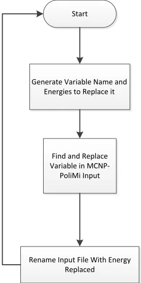
3.5 Creating Input Files and Running Script on 32 CPUs
To expedite running forty instances of MCNPX-PoliMi, input cards with an energy
energy (Figure 3.11) and run the MCNPX-PoliMi instance across 31 CPUs (Figure 3.12).
This dramatically reduces the effort and time required to collect these data.
Start
Generate Variable Name and Energies to Replace it
Find and Replace Variable in
MCNP-PoliMi Input
Rename Input File With Energy Replaced
Figure 3.12: Input Card Generating Algorithm
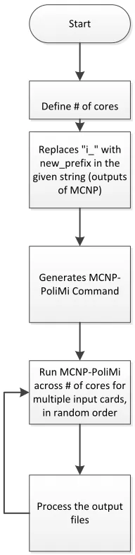
The algorithm for running all these instances of MCNPX-PoliMi defines the number of cores
and renames the outputs and log files with the corresponding input name. With this
information, the MCNPX-PoliMi run commands can be created and run across multiple cores
Start
Define # of cores
Replaces "i_" with new_prefix in the given string (outputs
of MCNP)
Generates MCNP-PoliMi Command
Run MCNP-PoliMi across # of cores for multiple input cards, in random order
Process the output files
Figure 3.13: Algorithm for running instances of MCNPX-PoliMi across N CPUs
3.6 Proving Radial Symmetry of the Detector
By using the 35 mm beam width, the count distribution across the detector was
established. Starting at the center and shifting the beam direction in 50 mm increments across
the entire detector face, the count distribution was analyzed (Figure 3.14, 3.15). The counts
Figure 3.14: Distribution of Pixel Counts in the Y Direction 30500 31000 31500 32000 32500 33000 33500 34000
-5 -4 -3 -2 -1 0
Co u n ts Position cm 31000 31500 32000 32500 33000 33500 34000
-5 -4 -3 -2 -1 0
Co
u
n
ts
Table 3.2: Count Error for Comparing X and Y Directions
Beam Distance from Center Point (cm)
Difference in X and Y Counts
Percent Difference
Std Dev Y Direction
Std Dev X Direction
0 0 0 1160 1160
0.25 0 0 1161 1161
0.75 456 0.033 1160 1160
1.25 651 0.048 1159 1159
1.75 2157 0.165 1156 1155
2.25 1887 0.144 1145 1144
2.75 1328 0.123 1086 1086
3.25 816 0.083 987 988
3.75 1047 0.128 903 902
4.25 2242 0.431 721 723
From Table 3.2, the percent difference between the x and y directions never reach 0.5%. This
allows the assumption that the x and y directions may be treated as a single radial dimension.
Figure 3.16 shows how the spectrum changes in the x direction with changing beam
distances from the center. As the beam is directed at an area farther from the center of the
detector, counts are lost by gamma rays escaping the boundary of the detector. Therefore, as
expected, the center point has the most counts and 4.25 cm from the center has the least
Figure 3.16: Spectral Changes with X-Position
Figure 3.17: Spectral Changes with Y-Position
To further prove the radial symmetry of the detector, spectra from the x and y
directions were interpolated to find the spectrum expected at a point between these two
directions. Conventional bilinear interpolation does not work in this case because we are
interpolating on a circular surface.
A method called SLERP, or Spherical Linear Interpolation, essentially takes two
vectors (the spectra in the x and y directions) and interpolates the rotation about these
vectors. The shortest path on this unit sphere can be scaled to the right magnitudes [11]. This
Figure 3.19: Linear Scale Comparing SLERP Method and MCNPX-PoliMi Direct
Calculation
These two figures show that the detector is radially symmetric because the SLERP values
coincide with MCNPX-PoliMi generated spectra in addition to the x and y directions
previously shown in Figures 3.16 and 3.17.
3.7 Interpolating Separate Features of the Spectrum
The MCNPX-PoliMi generated spectrum must be split into separate features based on
different photon interactions before the spectrum can be interpolated. Some features of
gamma spectra do not change linearly when the source energy is changed and therefore
show in Figure 3.20. The algorithm uses all the log files generated from the MCNPX-PoliMi
Start -Choose Filename -Import Class dumn_file End Class: dumn_file
Create New Object: self
-Parses the filename provided at object instantiation. - populate the self.energies and self.cube from PoliMi log
Class: detector
Computes the energy spectrum from the data contained in self.cube
Writes the energy spectrum for each feature to a .csv file
Uses matplotlib.pyplot to save a plot of the energy spectrum as a
.png file
Gets the cube subset specified and returns it
Converts from dumn-file coordinates to pixel
coordinates Define front and back
detector
New Particle?
NO YES
Which Feature?
The log files appear in the form of Figure 3.21. As mentioned before, this algorithm also
produces an image file that shows the detector face displaying where the most collisions
happened. The data columns used in this post-processing include: particle history number,
interaction type, cell number of collision event, collision position, and number of scatterings.
This information is extracted and put into one of three spectral feature categories: Compton
scattering, full energy peak, and the backscatter peak. These were saved as a list for use in
Matlab to be interpolated.
must collide in both the front and back parts of the detector to register a collision. When this
happens, the particle interaction type on the last collision, either an absorption or scatter (0 or
1), is noted. When it ends in a scatter event (1), it is a Compton feature. If it ends in
absorption, then this particle belongs to the full energy peak or backscatter category. To
determine which feature it belongs to, the value in the collision column is checked to
determine if it is monotonically increasing. If it is, this means all collisions occurred in the
sensing cells of the detector which makes it part of the full energy peak. If instead there is a
missing collision, then the particle had an interaction outside the sensing cells of the detector
but then scattered back into a sensing cell of the detector making it a backscatter feature.
Hits Front and Back Detector
NO
END
YES Does Particle History End in a 0(Capture)? NO New Particle History
Add Count to Compton Scatter
Are Numbers Monotonically Increasing?
NO Add Count to
Backscatter
YES Add Count to Full Energy Peak Start
YES
To interpolate each feature, the list files were loaded into MATLAB. The full energy peak,
backscatter, and Compton scattering were interpolated. First, the radial positions and energies
calculated are tabulated in a large array. The user inputs the desired radial position and
energy in the detector and MATLAB accesses the corrected lower and upper position and
energy spectra.
The x-coordinate for the interpolated full energy peak is the source energy. The ratio
of this energy to the x-coordinate of either the upper or lower spectrum full energy peak was
calculated. This number was used to multiply the entire upper or lower spectrum abscissa
(energy) values to yield a new interpolated spectrum.
To find the interpolated ordinate values (counts) of the spectrum, the line between the
upper and lower peaks is calculated using Equation 21 and shown in Figure 3.23.
Figure 3.23: Determining Interpolation Counts from Lower and Upper Spectra
Because two points on the line are known (the two peaks), the slope m for each feature can
be directly calculated using Equation 22 for the 3 separate features (full energy peak,
Compton edge/continuum, and backscatter peak).
1 2
1 2
y y
m
x x
(22)
The point-slope version was used, Equation 23, where m is the slope and ( ,x y1 1) is the
upper or lower spectrum peak and x is the known location of the full energy peak which in
this case is merely the source energy. The number of counts in the peak of the interpolated
y y1 m x( x1) (23)
From this, a ratio was found by dividing this y value by the y value of the counts at the peak
of either the lower or upper spectrum. This number is multiplied by all the y-values on the
newly x-interpolated spectrum from above. The interpolated spectrum is now defined.
This interpolation method was used for the backscatter and Compton scattering
features [33]. However, the location of the x-coordinate for the interpolated spectrum is
different for both of these features. For Compton scattering, Equation 5 is used and for
backscatter Equation 6 is used from Chapter 2. As a result of the new position, the continuum
is stretched to fit the new x-values.
Te,max E E',min (5)
' 2 2 1 e E E E m c (6)
Finally, the counts of the three spectra are summed to get the complete number of counts.
The average of the three spectra’s x-values was used for the energies of these counts on the
3.8 Re-binning Interpolated Energy Bins to MCNPX Energy Bins
In order to compare the interpolated spectra with the MCNPX PoliMi calculations,
the interpolated energy bins must be re-binned into the original 50 keV interval energy bins.
This allows the spectrum to be compared directly with the MCNPX-PoliMi calculated
spectrum that uses the 50 keV binning structure.
To re-bin the interpolated data, a script in Haskell was used [24]. In short, this script
takes advantage of the “sweep” style algorithm, which means it takes the x-coordinate data
and “sweeps” from left to right to calculate how many counts are in each new energy bin. It
creates a “number line” of each increasing bin and when they overlap, the counts are split
based on a linear weight based on the amount of overlap of the two bins. To clarify, the
contributions of each pixel are weighted.
To use this code, the user will input x1, y1, and x2 which correspond to the
interpolated spectrum x values (energy bins), the interpolated y values (counts), and the
desired MCNPX-PoliMi based binning, respectively. The sweep style algorithm can
determine the number of counts from the x1 bins that go into the new x2 bins based on how
Figure 3.24: Sweep-Style Re-binning Algorithm for Interpolated Bins (X1) and the
MCNPX-PoliMi Bins.
If x2 comes before the next x1 value, a fraction of the x1 counts will go into the first x2 bin
while the remaining fraction goes into the following x2 bin [25]. This assumes that the
energies are uniformly distributed in the bins.
Chapter 4: Results
4.1 Calculated Response Function
The response function that the interpolated method draws from should be in the form
of the figure in Chapter 2, Figure 2.11. This response function for the HPGe detector is
Figure 4.2: Response Function for the HPGe Strip detector at 0.25 cm Radius (Log Scale)
The plot follows a similar trend as the example with a full energy peak following the
diagonal. Similarly, if a radius closer to the edge of the detector was chosen, a plot with
fewer counts is expected. This is seen in Figure 4.3 and Figure 4.4 below with a radius of
Figure 4.4: Response Function for the HPGe Strip detector at 3.25 cm Radius (Log Scale)
The full energy peak from the photoelectric effect is the dominant feature in these spectra.
Since the Z value for Germanium is 32 and the energy range is from 0.05 to 0.5 MeV, the
graph below substantiates that the full energy peak from the photoelectric effect is indeed the
Figure 4.5: Dominating Photon Effects at Different Energy and in Different Material [28]
4.2 Single Energy and Radial Position Interpolated Spectra
A single source energy and radius not in the generated response function library was
interpolated and re-binned to prove this interpolation method is accurate. An energy of
0.1635 MeV and a radius of 2.00 cm was interpolated and then compared with the
MCNPX-PoliMi generated spectrum. The Compton edge and continuum begin at approximately 0.06
Figure 4.6: MCNPX-PoliMi Generated Spectrum vs Interpolated Spectrum Without
Figure 4.7: MCNPX-PoliMi Generated Spectrum vs Interpolated Spectrum Without
Re-binning, Log Scale
Notice in Figure 4.7 that the discontinuity at the Compton edge derives from the lack of
counts collected at this energy. Comparing the interpolated spectrum and the direct
calculation reveals that the spectra are very similar. After the interpolated spectrum was
re-binned, the final spectrum comparison is shown below for a single interpolated energy and
Figure 4.8: MCNPX-PoliMi Generated Spectrum vs Interpolated Spectrum with Re-binning,
Figure 4.9: MCNPX-PoliMi Generated Spectrum vs. Interpolated Spectrum with Re-binning,
Log Scale
The difference between re-binning is small but necessary to compare the MCNPX-PoliMi
calculation to the interpolated and re-binned spectrum. As expected, re-binning the data
resulted in the data being spread across more energy bins.
4.3 Ba-133 Decay Spectrum Using Interpolation Method
To verify that this is the correct response function for the HPGe strip detector and that
this interpolated and re-binning method is correct for generating a spectrum, a real source
spectrum from a radionuclide was compared to the MCNPX-PoliMi direct calculation of the
detector’s energy range (50-500 keV). The decay scheme and gamma ray energy and
intensities are given in Table 4.1 and Figure 4.10.
Table 4.1: Gamma Ray Energies and Intensities for 133Ba [26].
Gamma Ray Energy (keV) Gamma Ray Intensity (%)
53.1625 2.2
79.6139 2.6
80.9971 34
160.6109 0.64
223.2373 0.45
276.3997 7.16
302.851 18.3
356.0134 62
383.848 8.9
These nine energies were run separately in MCNPX-Polimi, multiplied by their intensity, and
then added together to get the full 133Ba decay spectrum (Figure 4.11 and Figure 4.12).
Figure 4.12: 133Ba Decay Spectrum Calculated Using MCNPX-PoliMi (Log Scale)
Figure 4.13 demonstrates the typical Ba-133 spectrum found in practice and these peaks
align correctly to the spectrum found in literature. The lowest energy peak, 0.053 MeV, does
not show up in MCNPX-PoliMi generated spectrum as much because the lower energy
photon does not have enough energy to strike both the front and back detector. If the photon
Figure 4.13: Germanium Spectrum of 133Ba [27]
The result of these interpolations, with only energy being interpolated and the radius being a
directly accessible in the library of interpolation data, is displayed in Figure 4.14 and Figure
Figure 4.14: 133Ba Spectrum Comparison with Interpolated and Re-binned Spectrum at a
Figure 4.15: 133Ba Spectrum Comparison with Interpolated and Re-binned Spectrum at a
Radius of 2.25cm on a Log Scale
The interpolated and re-binned spectrum closely follows the direct calculation. The spread of
the interpolated spectrum to the left of the 0.302 MeV energy was the result of the re-binning
algorithm where the binning boundary fell such that only a few counts fell into the 0.302
MeV peak. These plots with error bars, using a Poisson distribution (square root of the
Figure 4.16: 133Ba Spectrum Comparison with Interpolated and Rebinned Spectrum at a
Figure 4.17: 133Ba Spectrum Comparison with Interpolated and Rebinned Spectrum at a
Radius of 2.35 cm on a Log Scale, with Error Bars (Poisson)
The 133Ba spectrum was also compared with a radius that had to be interpolated (2.00cm).
This radial distance was not already one of the radii already calculated in the interpolation
Figure 4.18: 133Ba Spectrum Comparison with Interpolated and Rebinned Spectrum at a
Figure 4.19: 133Ba Spectrum Comparison with Interpolated and Re-binned Spectrum at a
Radius of 2.00 cm on a Log Scale
These spectra are very similar but follow the direct calculation less closely than the spectrum
where only energy was being interpolated. Since this interpolates both radius and energy, the
results are not as accurate since there are now two dimensions interpolated. Again, the
spreading issue at the 0.302 MeV peak is a result of the rebinning algorithm where the
interpolated and MCNPX-PoliMi bin values greatly overlapped resulting in only a few
counts making it to the bin that contains the 0.302 MeV peak. These results with error bars,
Figure 4.20: 133Ba Spectrum Comparison with Interpolated and Re-binned Spectrum at a
Figure 4.21: 133Ba Spectrum Comparison with Interpolated and Re-binned Spectrum at a
Chapter 5: Conclusions
This work on HPGe strip-type detector/imager has far reaching effects in many fields,
especially in applications for homeland security and medical imaging. Position sensitive
HPGe imagers like this give not only superior energy resolution with the gamma ray
spectrum, but also information pertaining to the coordinates of the measured source. This
project characterizes this type of detector using a model built in MCNPX PoliMi. The
detector was determined to be radially symmetric in gamma ray counts. The generated
photon interaction log was analyzed by photon features to create a detector response function
versus radial position using 40 mono-energetic sources. These gamma ray spectra were then
interpolated to create a detector response function that could be used to interpolate the
response to an arbitrary source spectrum.
The main findings suggest that the single source energy interpolated spectrum in both
the energy and radial position dimensions closely match the spectra directly calculated using
MCNPX-PoliMi (Figures 4.8 and 4.9), showing this interpolation method is valid in this
case. When comparing the Ba-133 decay spectrum in literature to that in the MCNPX PoliMi
direct calculation for this detector setup (Figures 4.12 and 4.13), there were some notable
differences. Namely, the lower gamma-ray energy at 0.053 MeV does not have enough
energy to strike the front and back electrodes of the detector, therefore not registering a count
as seen in these Ba-133 decay spectra that are being compared.
follows the general shape of the direct calculation (Figures 4.16 and 4.17). Similarly, adding
the radial distance as an interpolation dimension yields a similar result with the interpolation
method following the general shape of the direct calculation, albeit with more error due to the
extra dimension being interpolated (Figures 4.20 and 4.21). Note that at the 0.302 MeV
gamma ray energy, the re-binning algorithm has spread the counts in bins to the left of the
actual direct calculation bin. Although this is rare, it can happen as a result of the sweep-style
binning algorithm (Figure 3.22) where it is possible to have minimal overlap in the correct
bin if the original bin structure falls in the new re-binning structure with only a few counts.
In order to expand on this research, a finer mesh of energy and pixels should be used.
This project was limited by computational time due to access of only 32 cpus. The time for
one MCNPX PoliMi run with one million particles took 5.61 minutes and with 40 energy
points and 18 radius distances, this would take over 2 hours on 32 cpus. This was a
reasonable amount of computational time on this project. However, since these counts are
Poisson distributed and calculated with Monte Carlo methods where confidence is increased
with more histories, decreasing the error by a factor of N requires the number of histories to
be increased by N2 which greatly increases computational time for small decreases in error.
A smaller error would increase the validity of these calculations since the interpolation
distances between energies and radii would be less coarse. In addition, experimental data
should be compared to the computational data generated in this project. During the course of
this research, the detector being studied was not available.
Overall, this research shows that by combining the detector symmetry in the radial
computational time can be hugely decreased compared to that of direct Monte Carlo
![Figure 2.1: Semi-Conductor Detector Mechanics [32]](https://thumb-us.123doks.com/thumbv2/123dok_us/1332327.1166196/17.612.97.539.74.430/figure-semi-conductor-detector-mechanics.webp)
![Figure 2.2: Gamma-Ray Spectrum Features [41]](https://thumb-us.123doks.com/thumbv2/123dok_us/1332327.1166196/21.612.119.526.101.361/figure-gamma-ray-spectrum-features.webp)
![Figure 2.3: Klein-Nishina Kernel [15]](https://thumb-us.123doks.com/thumbv2/123dok_us/1332327.1166196/23.612.167.459.149.433/figure-klein-nishina-kernel.webp)
![Figure 2.4: Compton Continuum Shape [15]](https://thumb-us.123doks.com/thumbv2/123dok_us/1332327.1166196/24.612.173.462.67.440/figure-compton-continuum-shape.webp)
![Figure 2.6: Pinhole Camera Diagram [35]](https://thumb-us.123doks.com/thumbv2/123dok_us/1332327.1166196/29.612.224.442.291.536/figure-pinhole-camera-diagram.webp)
![Figure 2.7: A Uniformly Redundant Array Coded Aperture [23]](https://thumb-us.123doks.com/thumbv2/123dok_us/1332327.1166196/30.612.244.421.372.544/figure-uniformly-redundant-array-coded-aperture.webp)