The Application of Bayesian Hierarchical Models
to Heterogeneous DNA Profiling Data
Thesis submitted to the University of London for the degree
of Doctor of Philosophy in the Faculty of Science
by
John Pueschel
Department of Statistical Science
University College London
ProQ uest Number: 10014978
All rights reserved
INFORMATION TO ALL U SE R S
The quality of this reproduction is d ep en d en t upon the quality of the copy subm itted. In the unlikely even t that the author did not sen d a com plete manuscript
and there are m issing p a g e s, th e se will be noted. Also, if material had to be rem oved, a note will indicate the deletion.
uest.
ProQ uest 10014978
Published by ProQ uest LLC(2016). Copyright of the Dissertation is held by the Author. All rights reserved.
This work is protected against unauthorized copying under Title 17, United S ta tes C ode. Microform Edition © ProQ uest LLC.
ProQ uest LLC
789 East E isenhow er Parkway P.O. Box 1346
Abstract
A situation is considered in which a suspect has been found whose DNA profile matches that of a sample, assumed to originate from the offender, found at the scene of a crime being investigated.
The way in which this evidence should be used is reviewed, high lighting the role of the match probability, the probability of a particular individual having the profile in question given the suspect’s possession of the profile, and a database of individual profiles. The value of this prob ability is affected by the heterogeneity of the population, and failure to take account of this could result in a false conviction.
A Bayesian hierarchical model designed to represent population sub structure is presented. Parameters are clearly defined at each level within a model displaying justifiable conditional independence properties. This model is then used as a basis for inference about the required match probabilities, highlighting errors in previous approaches.
A ck n ow led gem en ts
I would especially like to express my gratitude to Professor Phil Dawid for his excellent guidance, encouragement and patience.
The financial support provided by EPSRC is also much appreciated.
I would also like to thank many other members of the Departm ent for their help and encouragement, in particular fellow members of the research student group, and the undergraduates who ‘dared’ to enter our room. I would like to mention you all by name, but fear th at I would miss someone. You know who you are, and the friendships developed are truly valued.
Various other people require thanking for keeping me (relatively) sane, in cluding the Marshalls crew, the football lads, Ryz, Andy and Dave.
C ontents
1 In tro d u ctio n 10
1.1 B a c k g ro u n d ... 10
2 M eth o d s o f m atch p ro b a b ility calcu lation 15 2.1 Product r u l e ... 15
2.2 Taking account of population s u b s tr u c tu r e ... 16
3 T h e H ierarchical M od el 23 3.1 In tro d u c tio n ... 23
3.1.1 E x changeability ... 23
3.2 Outline of the m o d e l ... 24
3.3 Introducing extra levels to hierarchical m o d e ls ... 27
4 Inference 35 4.1 In tro d u c tio n ... 35
4.1.1 Model I ... 36
4.1.2 Model I I ... 38
4.2 Inference under the two m o d e l s ... 39
4.3 Inference under unknown individual subpopulation labels . . . . 43
4.4 Markov chain Monte C a r lo ... 44
5 M easu res o f su b p op u lation d ifferentiation 45 5.1 N e i ... 46
5.2 Weir and C o c k e rh a m ... 47
5.3 How are the measures of subpopulation differentiation related? . 48 6 M arkov chain M on te Carlo m eth od s 50 6.1 In tro d u c tio n ... 50
6.2 Markov c h a in s ... 51
6.3 Metropolis-Hastings a lg o rith m ... 53
6.4 Gibbs s a m p lin g ... 55
6.5 Hybrid MCMC schemes ... 56
6.6 Techniques to improve m ix in g ... 56
6.7 Simulated te m p e r in g ... 56
6.8 Im portance s a m p lin g ... 58
7 A p p lica tio n o f M arkov chain M on te Carlo 60 7.1 In tro d u c tio n ... 60
7.2 Subpopulation labels k n o w n ... 61
7.3 Subpopulation labels u n k now n ... 69
8 T h e d efin itio n o f a sub p op u lation , and its effects 71 8.1 In tro d u c tio n ... 71
8.2 A n a ly s is ... 74
8.2.1 Assumptions regarding subpopulation membership of cul prit C and suspect s ... 76
8.3 Individual subpopulation labels k n o w n ... 77
8.4 Labels u n k n o w n ... 80
8.4.1 Subpopulation proportions assumed k n o w n ... 82
8.4.2 Subpopulation proportions assumed u n k n o w n ... 93
9 A lte r n a tiv e m eth o d s 107 9.1 In tro d u c tio n ... 107
9.2 Roeder, Escobar, Kadane and B a l a z s ... 107
9.3 Foreman, Evett and S m i t h ... 110
9.3.1 C i V s ... 113
9.3.2 C ^ V s... 114
9.4 D isc u ssio n ... 115
10 F u ture w^ork 125 10.1 Variable number of s u b p o p u la tio n s ... 126
10.3 Application of Bayesian methods in the c o u rtro o m ... 128
10.4 Presentation of the e v id e n c e ... 129
10.5 A critical a n a ly s is... 131
10.6 Adjusting the m o d e l ... 135
10.7 S u m m a r y ... 135
A B io lo g ica l background 142
B D eriv a tio n o f th e full con d ition al d en sity o f a 144
List o f Tables
1 Comparison of third centralised moments of 1 and 2 stage models. . 33
2 Comparison of fourth centralised moments of 1 and 2 stage models. . 33
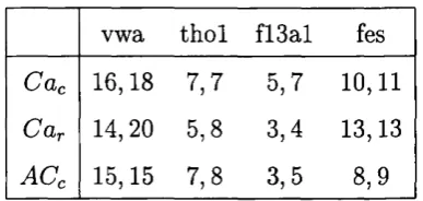
3 Suspect profiles used for analysis... 75
4 Posterior match probabilities for profile Cac... 78
5 Posterior match probabilities for profile Car... 79
6 Posterior match probabilities for profile ACc... 79
7 Individual locus posterior match probabilities for profile ACc... 80
8 Posterior match probability estimates when k is known... 82
9 Posterior match probabilities when k is known, employing simulated tempering... 92
10 Posterior match probabilities when k, ~ Dirichlet 11 Posterior match probabilities when k ~ Dirichlet 12 Posterior match probabilities when k ~ Dirichlet 13 Posterior match probabilities when k ~ Dirichlet 14 Posterior match probabilities when k, ~ Dirichlet 15 Posterior match probabilities when k ~ Dirichlet 16 Posterior match probabilities when k. ~ Dirichlet ( 17 Quantités of the posterior distribution of the overall match probability. 105 18 Posterior probabilities of guilt for an individual with profile ACc under a range of prior probabilities of guilt... 106
1,1)... 96
7.3 )... 96
70.30 )... 97
700.300 )... 97
7.3 )... 103
70.30 )... 104
List o f Figures
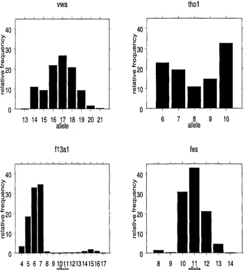
1 Relative frequency graphs of alleles in a Caucasian database... 11
2 Population substructure model... 17
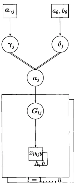
3 DAG outlining basic model... 25
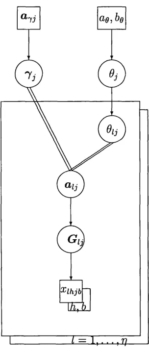
4 DAG showing subpopulation specific differentiation parameters. . . . 28
5 DAG for the case of complete information... 37
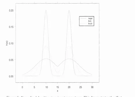
6 Normalized densities at various temperatures... 57
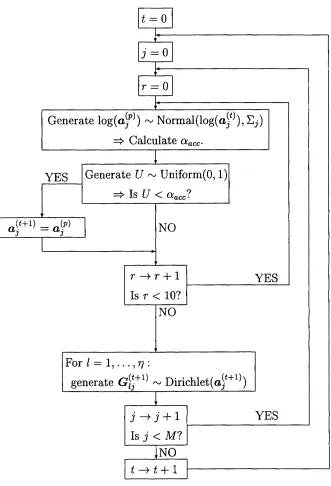
7 Flow diagram representing MCMC scheme... 67
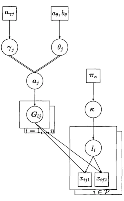
8 DAG for the case of incomplete information... 70
9 Trace of (713(6) initialised by 7 different random seeds... 83
10 Allocation of individuals: « known, random seed = 12... 84
11 Allocation of individuals: k known, random seed = 1... 84
12 Allocation within the two posterior modes... 85
13 Comparison of log likelihood... 8 6 14 DAG for the case of incomplete information, including ‘mixing’ vari able S... 89
15 Traces of simulated tempering level and an allele frequency... 92
16 Prior densities for k(1)... 95
17 Individual allocation: k ~ Dirichlet(1,1), random seed = 12... 98
18 Individual allocation: k ~ Dirichlet(1,1), random seed = .1... 98
19 Individual allocation: k ~ Dirichlet(7,3), random seed = 12... 99
20 Individual allocation: k ~ Dirichlet(7,3), random seed = .1... 99
21 Individual allocation: /c ~ Dirichlet(70,30), random seed = 12. . . . 99
22 Individual allocation: k. ~ Dirichlet(70,30), random seed =.1... 100
23 Individual allocation: k, ~ Dirichlet(700,300), random seed = 12. . . 100
24 Individual allocation: k, ~ Dirichlet(700,300), random seed = 1. . . . 100
25 Comparison of log likelihood ratios for Caucasian individuals... 117
26 Comparison of log likelihood ratios for Afro-Caribbean individuals. . 117
29 Comparison of posterior probabilities of guilt, tts = 10"'^, 6j = 0.0. . 121
30 Comparison of posterior probabilities of guilt, tts = 10~'^... 121
31 Comparison of posterior probabilities of guilt, tts = 10“ ®, 9j = 0.0291. 122 32 Comparison of posterior probabilities of guilt, tTs = 10“ ®, 6j = 0.01. . 122
33 Comparison of posterior probabilities of guilt, tts = 10“ ®, 9j = 0.0. . 123
34 Comparison of posterior probabilities of guilt, tts = 10“ ®... 123
35 Caucasian database... 146
36 Afro-Caribbean database... 147
1
Introduction
1.1
Background
Over the past ten years, ‘DNA fingerprinting’ has become an im portant tool in the legal world. High profile cases such as the O.J. Simpson trial [Weir, 1995] have increased public awareness of the technique.
At any criminal trial, the ultim ate aim is to reach a decision regarding the guilt of the defendant. It has been argued [Fienberg and Finkelstein, 1996] th a t Bayesian methods provide a sensible framework for reaching this decision. The application of such a method would result in a posterior probability of guilt of the suspect given the evidence. The suspect would then be convicted if this probability is above a certain value.
A DNA profile consists of pairs of observations, one at each of a small number of well defined sites, or loci One member of each pair is inherited from the individual’s father, and one from the mother. The possible observations at each locus are referred to as alleles, each effectively representing a number of repeats of a sequence of base pairs (see Appendix A for further detail).
For our purposes, a DNA profile takes the form of a series of pairs of inte gers, one pair for each locus considered, each number representing a different allele. The empirical frequencies of various alleles at four loci within a Cau casian database can be seen in Figure 1. W ithin this population, the profile {(16,17)(7,10)(5,7)(11,11)} would be considered a relatively common profile, while {(13,20)(5,8)(8,8)(8,9)} is a rare profile.
In this thesis we consider a situation in which a crime has been committed and a tissue sample (possibly blood, hair, semen, etc.) has been recovered from the scene. From this sample we have a DNA profile X c assumed to be th a t of the culprit C.
In addition we have a suspect s whose DNA profile X s is found to match
X c - We denote the known matching profile by y.
vwa
tho1
13 14 15 16 17 18 19 20 21
allele 6 7 allele8 9 10
fISal
fes
4 5 6 7 8 9 1011121314151617
allele
' I I
8 9 10 11 12 13 14
allele
Figure 1: Relative frequency graphs of alleles in a Caucasian database.
comprise a number of suspects, some of their close relatives, a database of kno'wn criminals and a “statistical” database drawn from the general population. We restrict ourselves to the instance in which â represents a statistical database. The collection of DNA profiles from these individuals is labelled Xâ- O ther (non-DNA) evidence, such as eye witness accounts or alibis, which may appear to be for or against the suspect, is labelled e.
all the evidence and d ata available
Pguilt Pr(C7 = s| ^ C ~ ^ s ~ y ^ X ô — ^<îj
^)-Application of Bayes’ Theorem allows this probability to be expressed [Dawid and Mortera, 1996, Weir, 1994] as
where
— Pr((7 = — y^XS ~
— P r ( xc ~ y \ c ~ -Xs ~ y 1 Xs )
i labels individuals, and V represents the population of possible culprits.
W ithout knowledge of the culprit profile X c , it is reasonable to assume th a t C is independent of (X s,^ j). In this thesis we assume th a t the sample X c is definitely th at of the culprit, and th at there are no errors in the process establishing a profile from a sample. In reality this is not necessarily so, but these assumptions allow us to take rris to be 1, and simplify equation (1) to give
where
7Ti = P r(C = zle),
— Pl^(Xc — y \ C — Z, X a = y, Xs —
^)-A priori the members of the database are potential perpetrators. It is as sumed th a t the DNA profile measurements contain no error, and it is therefore possible to eliminate any database individual whose profile does not match y.
where j3 is the set of individuals in the complete database a whose profiles m atch the profile y of the culprit.
To evaluate (3), prior probabilities of guilt must be specified for each indi vidual. In particular, members of the jury use the non-DNA evidence to arrive at a subjective prior probability tts of guilt of the suspect. Match probabili ties can then be used to update these prior probabilities, leading to a posterior probability of guilt for the suspect.
A major problem faced is th at of evaluating a match probability for each of a potentially large number of individuals in the suspect population V.
The calculation of a match probability for each individual in the population is impracticable.
Some methods previously employed have calculated a single match probabil ity for all the individuals. These methods, described in Chapter 2, do not take reasonable account of genetic relationships between individuals. In Chapter 2 we consider why it it is im portant to take account of these relationships, and consider how this might be achieved. Chapter 3 introduces a hierarchical model designed to incorporate population substructure. In Chapter 4 we consider how this hierarchical model can be used to define two statistical models, and how these can be used to calculate the required match probabilities. The hierarchi cal model provides a framework which is used in Chapter 5 to clearly define the roles of various genetic parameters.
As the calculations required to evaluate match probabilities are impossible analytically, Markov Chain Monte Carlo methods are introduced in Chapter 6 as a precursor to their application in Chapter 7.
O ther authors, in particular Foreman, Evett and Smith
th a t the approach of this thesis represents a step forward, match probabilities and posterior probabilities of guilt are calculated under the various methods described, and compared.
2
M ethods o f m atch probability calculation
To calculate a posterior probability of guilt for the suspect we require a match probability rrii for each individual i in the population V:
— y \ ^ s — 2/j X.5 — ^5 i
^)-Frequently close relatives of the suspect can be eliminated from the enquiry. If they cannot be eliminated, it is im portant th at they be included in the calcu lation. If it is impossible to obtain a DNA profile from a close relative, then the match probability of th at individual should be calculated separately. Two indi viduals having recent ancestors in common have a greatly increased probability of inheriting common genes. This means th at, for a close relative of the suspect, the probability th a t they have the profile y given th a t X s = y will generally be much higher than for unrelated members of the population, reducing the weight of evidence against the suspect. Derivation of close family match probabilities is described by Donnelly [Donnelly, 1995].
For the remainder of the thesis we concentrate upon methods for match probability calculation for members of the general population.
In this chapter we consider methods of match probability calculation previ ously presented in court. The errors in these methods are highlighted, leading to an outline of the philosophy employed in this thesis.
2.1
P rod u ct rule
The initial method used to calculate the match probability of the offender em ployed the product rule [NRC, 1996].
We define gj{k) as the relative frequency of allele k at locus {j = 1 , . . . , M )
within the population under consideration. Under the product rule, the match probability is then defined as
M
rrii = n (4)
h{r, s) = <
where yjb refers to allele b of the pair observed at locus j of the suspect profile, and
0 if r = 5;
1 if r ^ s. for all individuals i.
This is estim ated by substituting empirical relative frequency estimates from a suitable database into the product in equation (4).
Derivation of equation (4) requires the assumption of independence of profile alleles across loci. To accept this method, one must also consider m ating to be random across the whole population. This is not a valid assumption, and its use can result in prejudice against the suspect.
2.2
Taking account o f p opulation substru ctu re
W ithin a large population, mating cannot be considered random. Individuals within sections of the population are more likely to m ate with another individual in th a t section than with someone outside it.
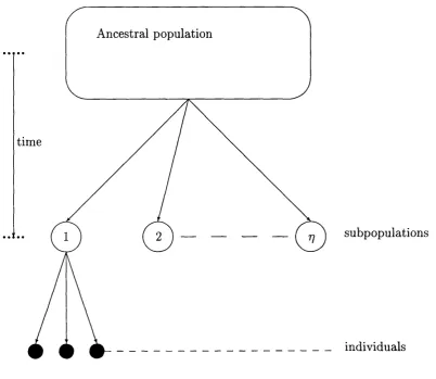
We approximate this situation with a model which divides the population into discrete subpopulations within which individuals are considered randomly mating. These subpopulations are considered to have evolved from a large an cestral population, as outlined in Figure 2.
One interpretation of these subpopulations within, say, an American Cau casian population would be as groups of people whose ancestors came from various countries of Europe. More usually, however, these subpopulations are mere artifacts of the model, designed to reflect the fact th a t individuals within a large population do not m ate at random. It is thus difficult to clearly define these subpopulations, and to allocate individuals to them in the way th at we could allocate, say, by nationality.
Ancestral population
time
subpopulations
individuals
The ceiling principle was designed to give a deliberately conservative estim ate of the match probability, i.e. greater than the true value. Its execution involves the use of samples from a number of subpopulations and for each allele taking the highest frequency among the groups sampled, or 5%, whichever is larger. The bound on the profile frequency is then obtained by multiplying together these individual allele limits. As the subpopulations are not usually clearly defined in terms of observable characteristics, it is difficult to obtain the samples required.
As a result of this difficulty, the interim ceiling principle was developed. This has been widely used. The rule states th a t “In applying the m ultiplication [of frequencies across loci] rule, the 95% upper confidence limit of the frequency of each allele should be calculated for separate ‘racial’ groups and the highest of these values or 10% (whichever is larger) should be used. D ata on at least three major ‘races’ should be analyzed.” The ceiling principle has been heavily criticized [NRC, 1996]. A clear flaw in the interim ceiling principle is th a t it will give the same limit regardless of the racial group of the individual concerned.
Weir [Weir, 1994] introduced a method far more satisfactory than the ceiling principle. Relating posterior odds to prior odds in the manner outlined in Chap ter 1, he too stressed the need to take into account the dependence between the
profiles of culprit and suspect when calculating m atch probabilities.
Wright [Wright, 1951] introduced parameters Fs t: Fi t and Fis to summarise
substructure within a population. They are defined as the correlations of genes of different individuals in the same subpopulation, of genes within individuals and of genes within individuals within populations respectively. This definition of “correlations” is unclear as when defining correlations it is necessary to be clear upon what we are conditioning. Population structure can be considered to be of a hierarchical nature (Figure 2). Assuming such a structure, statem ents of
are not equivalent. This further clouds the study of population substructure and is discussed in more detail in Chapter 5.
However the principle of introducing a param eter to govern subpopulation differentiation within the above model is a very im portant one. Weir [Weir, 1994] considered the effects of inbreeding on forensic calculations using this param eter based method.
Two genes at a locus are defined as being identical by descent (ibd) if they have the same ancestral gene. Weir defines a number of measures of descent affecting the probabilities of observing a particular set of four genes within two pairs. These include
0 the probability th a t any two genes at a locus are ibd;
7 the probability th a t any three genes are ibd;
6 the probability th a t any four genes are ibd;
A the probability th a t any two pairs of genes are ibd.
Single locus match probabilities
rrii = = { y i , y 2 ) \ X s = (?/i, 2/2), 7, A)
when the individuals i and s are assumed to belong to the same subpopulation are derived to be
[(1 — 6^ + 8 7 + 3A - 6ô)pi
+6(0 - 2 7 - A + 26)pi if yi = 2/2
+ ( 4 7 + 3A - 75)pi + (5] / [pi + (1 - Pi)9] ;
rrii = (5)
[(1 - 60 + 8 7 + 3A - dô)piPj
+2(0 — 2 7 — A + 20){pi + pj) if yji ^ yj2 + 2 ( A - ( ^ ) ] / ( l - 0 ) .
If the population under consideration is in evolutionary equilibrium, the quantities 0, 7, 6 and A are not changing over the time. Li [Li, 1996] showed
th a t in this instance 7, 6, and A can be expressed in terms of 0: 20^
7 =
602
à =
A =
(l + 0) (l + 2 0)
^2 (1 + 5^)
(l + 0) (l + 2 0)
Substituting these expressions into the conditional probabilities (5) gives expres sions in terms of 0 and population-wide allele frequencies 7 . These are similar in
form to those determined by Balding and Nichols [Balding and Nichols, 1995]. If, at a particular locus, the matching gene pair is homozygous (i.e. the two alleles displayed are similar),
(2 0 + ( 1 - 0)7 (î/i))(3 0 + ( 1 - 0)7 (î/i))
( l + 0 ) ( l + 20) ’
and if it is heterozygous,
_ „ (0 + (1 - 0)7(01)) + (1 -
8)y{y2))
(l + 0) (l + 2 0) ^ ^
Weir and Evett [Weir and Evett, 1998] discuss methods of estim ating the coancestry coefficient 6 given data from a number of subpopulations. However, because of the difficulty in allocating individuals to subpopulations, they suggest two possible alternatives to the problem of estimating match probabilities taking into account population substructure.
The first is to refer to previous studies of human population structure such as th a t by Cavalli-Sforza et al [Cavalli-Sforza et al, 1994]. Assuming th a t popu lations similar to th at under consideration have been studied, appropriate esti m ates can be substituted into equations 6 and 7.
The other alternative covered was proposed in the second NRC report [NRC, 1996] which was produced following heavy criticism of the ceiling principle and other aspects of the initial report. The NRC recommended the substitution
0Î9 = 0.03 into equations (6) and (7) when suspect and culprit are considered to
come from the same subpopulation. This is larger than most empirical estimates meaning th a t the resultant match probability estimates should be conservative.
about the posterior distribution of 6 conditional upon a database of individual profiles. The problem of a lack of subpopulation d ata is overcome by allowing the individuals to be partitiioned into a specified number of groups, their like lihood assigning most weight to those partitions grouping individuals with the most similar profiles. The results are then combined with the theory of Balding and Nichols to produce match probability estimates in the presence of popula tion substructure. The paper of Foreman et al is discussed in more detail in Chapter 9. It proposes the calculation of two match probabilities, one condi tional on the suspect being in the same subpopulation as the culprit, and one conditional on the two being in different subpopulations. In this thesis we calcu late r) match probabilities, each conditional on the suspect being in a particular subpopulation (Vi; / = 1, . . . , 77).
As random mating is assumed within each subpopulation, all individ uals within a particular subpopulation are considered to be exchangeable [Dawid and Mortera, 1996]. This means th at
P r ( X i = y \ X a = (8)
is constant for all individuals i (outside the database a) in subpopulation Vi.
This probability will be referred to as the subpopulation match probability mi.
Assuming th at there are 77 subpopulations, the denominator of the posterior
probability of guilt of the suspect (equation (3)) becomes
^ 7T^ -H P r(C 0 a) ^ AfTTTf, (9)
ie/3 1=1
where A, = P r(C e Vi\C ^ a).
Calculation of the subpopulation match probabilities (mi] I = 1, . . . , 77) is
based upon the Bayesian hierarchical model outlined in Chapter 3 and is de scribed in detail in Chapter 4.
3
The Hierarchical M odel
3.1
In troduction
The population model described in Chapter 2 displays a clear hierarchical stuc-
ture with the following three levels:
(i) ancestral population;
(ii) subpopulations, descended from the ancestral population;
(iii) individuals, within the subpopulations.
3.1.1 E xch an geab ility
Assumptions of exchangeability feature heavily in this model. Variables
X i , . . . , X n are considered exchangeable if their joint probability distribution
f { x i , . . . ,Xn) is invariant to perm utations of the indices, i.e. there is no in formation conveyed by the unit indices themselves.
We assume th at, before observing any data, we have no way of distinguishing subpopulations, or individuals within subpopulations. We therefore apply the assumption of exchangeability to the units at stages (ii) and (iii) of the above model.
It is generally appropriate to model exchangeable variables as independently and identically distributed (iid) given some unknown param eter 6, say, with some distribution p{9). This arises from de Finetti’s theorem which states th a t in the lim it as n —>• oo, any suitably well-behaved exchangeable distribution on
( x i , . . . , Xn) can be w ritten in the iid mixture form p(æ) = j
-2 = 1
p{6)d9.
The structure and exchangeability properties assumed mean th a t the pop ulation model described is readily translated to a Bayesian hierarchical model involving param eters th at can be interpreted in terms of genetic characteristics.
3.2
O utline o f th e m odel
The profile X i of an individual i is a collection of genotypes, one at each of M
loci. The genotype at locus j consists of a pair of values from a finite set IZj of alleles. The set I tj consists of Vj consecutive integers, and at this point we map this series onto the sequence ( 1, . . . , rj). One member of the pair (the paternal
hand) is inherited from the father, the other (maternal band) from the mother. Generally we would not know which of the pair was the paternal band. However, as it simplifies the notation while making no difference with regard to inference from the database profiles, we consider the paternal and m aternal bands to be distinguishable. These bands are labelled by 6 = 1 (paternal), 2 (maternal). It is
im portant to note th at, when considering a match between the crime sample and the suspect s or a ‘random ’ individual z, we must take account of the fact th a t the bands are not truly distinguishable when calculating match probabilities.
The full DNA profile for individual i is
X i = {Xijb\j = 1, . . . , M; 6 = 1, 2}.
However, during this chapter, when describing the model we assume th a t the subpopulation of each individual is known. This allows us to define an alternative notation, replacing Xiji by Xihjb representing band b at locus j of individual h within subpopulation I.
We consider a heterogeneous population, consisting of (large) subpopulations labelled by / = 1 , . . . , 77, and propose the following 3-stage hierarchical model:
S ta g e 1 It is assumed that, conditional on some collection { G =
(Gij[l) , . . . , Gij{rj))] / = 1, . . . , 77; j = 1 , . . . , M } of “within-population” param e
ter vectors, there is independence of the values {Xijb) across bands within a pair, across loci, and across individuals. We then have, for each individual i e Vi
PT{Xihjb = k\G) = Gij{k), independently for all {h,j, b, I). (10) W ith reference to the “genetic model” described earlier, Gij{k) could be inter preted as a limiting relative frequency of allele k at locus j in subpopulation Vi,
if the size of th a t subpopulation tends to infinity.
S ta g e 2 As we consider the subpopulations exchangeable, it is appropriate,
at a fixed locus j , to treat [Gij] I = 1, . . . , 77) as independently and identically
distributed given some distribution II.
The distributon II can be chosen based upon a genetic model, such as th at described by Balding and Nichols [Balding and Nichols, 1994, Balding and Nichols, 1995]. At this point we introduce param eters {9j,7^), both
with a genetic interpretation at the ancestral population level. We consider 7^
to be a probability vector representing the mean, at locus j , of the process gener ating subpopulation allele probabilities. To govern the variance of this process, we define 9j. Such subpopulation differentiation param eters are mentioned fre quently in population genetics literature and are discussed further in Chapter 5. Assuming th at the model of Balding and Nichols is reasonable, there is some justification for the use, for IT, of the Dirichlet distribution:
Gij ~ D irichlet(aj(l), aj{2) , . . . , aj{rj)), independently for all /, j, (11) conditionally on hyperparameters (oj(l), Uj(2) , . . . , aj{rj)), where aj =
Under this distribution,
where % (+ ) = The variance of the subpopulation probabilities generated is then given by
= Sj'fj(.k){l ~ jj{k)). (13)
S ta g e 3 Finally, we need to give a distribution to II (or, equivalently, to (7 ,6)).
Assuming 7 and 0 to be independent, a reasonable prior for a would be based
upon
7j ~ Dirichlet{a^j{l),.. . ,a^j{rj));
6j ~ Beta(ug,6g);
where (aj^ag^be) are hyperparameters to be chosen.
This model can be used as a reference point for a discussion of the pub lished methods of tackling the problem of DNA identification using heterogenous databases. Of particular interest in a number of studies is the param eter describ ing subpopulation differentiation. In this instance, 0 is a param eter controlling the variance of allele frequencies generated. An alternative param eter could be defined to summarise the variation actually observed in the subpopulations 1 to
V-In many cases such parameters are confused and interchanged. Chapter 5 compares these parameters and clearly distinguishes them using the hierarchical framework outlined in this chapter.
3.3
Introducing extra levels to hierarchical m odels
It has been suggested th a t subpopulation specific differentiation parameters
[9i\l = 1,...,??) should be used. This adds an extra level of complexity to the model, but could be justified if it gives greater flexibility.
outline the m ethod we initially consider a similar model with Normal distribu tions, and then go on to consider the model described in this chapter.
It should be noted th a t adding extra levels of complexity to a hierarchical model does not necessarily result in a more flexible final model. An example is provided by the following model;
S tage 1
i = 1 , . . . ^ Normal(m/, cr^), independently across I.
S tage 2
mil/j,, ~ Normal(yU, r^), independently across I.
Assuming a, // and r to be known, this 2 stage model can be expressed as follows:
A/ = m/ -t- aZi
where {Zi) is defined to be a collection of independent standard Normal random variables, also independent of {mi)]
mi = 11 + tWi
where (Wi) is also a collection of independent standard Normal random variables. Then
A/ = f i + { a Z i + tWi)^
A/ ~ Normal()U, -f cj^)
independently across /, i.e. this two stage model can be expressed as a one stage model in which (A;) is a collection of independent and identically distributed variables with specified mean and variance.
If we now consider the following ‘extra’ levels as a potential extension to the hierarchical model introduced in this chapter (at this point simplifying by considering a univariate Gi for each subpopulation (Vi] / = 1, . . . , 77) and a single
locus):
S tage 1
GiKOi-z = 1 , . . . , 77,7) Beta ^ “ ^ 7 , ~ 7)1 , (14)
independently across {l]l = 1, . . . , 77).
S tage 2
6i\6 Bei3i{k6,k{l — 6)), (15) independently across I, where k is a fixed parameter. The density of G{=
(Gi,... ,Gr j)) is given by
/ ( G |e ,7 ) = I f i G \ 0 , 0 , j ) . n { 0 \ e ) d 9 i . . . d e ^
= / n / ( G 'l l f t , 7). n ^ W 9 ) d 0 i ■■■d9^
The probability density function of G conditional upon ^ is a product of identical terms, one for each subpopulation /, i.e. the subpopulation allele fre quencies {Gi, . . . , Gr,) are independent and identically distributed.
This is to be compared with the simpler model originally introduced:
G/16>,7 ~ Beta ~ y ~ ( l “ 7) j
The thinking behind the introduction of the extra level in the hierarchy is th at it increases the flexibility of the model, and th a t it reflects more closely the population substructure exhibited in the ‘real world’. However, it can be seen th a t the form of the model is essentially unchanged. In both cases, con ditional upon (0,7), the random variables (G^) are independent and identically
distributed.
Adding the extra level will lead to a greater degree of complexity in the model, increasing the difficulty in calculating results of interest. It is therefore appropriate to fully establish its necessity before including it in the model to be used as a basis for calculations within this thesis.
The conditional expectation and variance of Gi given (0 ,7) are calculated as
follows:
E[G,|7,^] = E[E[G,|^z, 7,^117,^] = E[7|7,0]
= 7. (16)
Var(G/|7,0) = E[var(G/|^z, 7,0)|7, 0]
+var(E[Gi|0;,7,6>]|7,6>]
= E[6a{l - 7) I7, e] + var(7|7,9)
= M l - 7). (17)
This means th a t the parameters of the simpler model can be selected to give a conditional mean and variance of Gi equal to the those of the ‘extra level’ model. This is also true of the multivariate case in which the Beta distribution of equation (14) is replaced by
Gi - Dirichlet ^ ^ ^ ^ 7 (1), ^ ^ ^ 7(2) , . . . , ~ ^ 7 ( 0 ^
The third and fourth central moments of the more complicated model are as follows;
E[ ( G/ — 7)^17, = E[Gf — 8 7^^ + 37^G /— 7^|7, 0] (18)
E[(G; — 7)^17, = E[Gf — 47Gf + 6 7^Gf — 47^Gz + 7^|7, (19)
The conditional expectation of Gi given (7,6) is known to be equal under
both models (16), as is the conditional expectation of Of (17).
E[Gf\^,6] and E[Gf|7, 0] can be evaluated exactly under the single level
model and approximated under the two level model:
_
^ 7((1 ~ ^1)1 + 0f)((l ~ ^/)7 + 2^z)~ [ (1 + 0/)
= E [ 7 ( ( l- % ) 7 + % ) ( ( l - 0 ,) 7 + 2 0;)
|7,0
x ( l ~ 0/ + 0f ~ 0? + • • -)|7 ,0]*
Similarly,
E[G?|7,0] = E[E[G3|%,7,0,]
X ((1 — 0 ^ )7 + 30/)(1 — 20/ + 40f — 80f + . . . I7, 0].
Non-centralised moments of 0/ are known for given (0,7) under the Beta
distribution of equation 15. Expanding these expressions up to 0" (for a chosen value of n), the moments can be approximated for chosen values of 0, 7. The
use of such approximations is justified by the fact th a t 0/ is known to be close
to zero.
Similarly to Foreman at al [Foreman, Evett and Smith, 1997], we have used values of k and 0 which give a conservative prior distribution for 0/ (i.e. giving
a higher probability density to values of 0/ greater than we would expect based
on previous studies).
k 9 7 E [(Q — 7 )^ 1 1 s t a g e m o d e l] E[{Gi - 7)5 12 s t a g e m o d e l] 5 0 0 . 0 2 5 0 .4 5 . 8 5 X 1 0-^ 9 . 9 7 X 1 0 - 5
1 0 0 0 . 0 2 5 0 .4 5 .8 5 X 1 0 - 5 7 . 9 7 X 1 0 - 5 5 0 0 . 0 2 5 0 .1 8 . 7 8 X 1 0 - 5 1 . 5 0 X 1 0 - 4
5 0 0 . 0 4 0 .1 2 .2 2 X 1 0 - 4 3 . 1 5 X 1 0 - 4
Table 1: Comparison of third centralised moments of 1 and 2 stage models.
k 9 7 E[{Gi - 7)4 |1 stage model] E[(Gi — 7)4[2 stage model]
50 0.025 0.4 1.04 X 10⁻⁴ 1.73 X 10⁻⁴
100 0.025 0.4 1.04 X 10⁻⁴ 1.40 X 10⁻⁴
50 0.025 0.1 1.95 X 10⁻⁵ 4.30 X 10⁻⁵
50 0.04 0.1 5.57 X 10⁻⁵ 9.82 X 10⁻⁵
Table 2: Comparison of fourth centralised moments of 1 and 2 stage models.
and fourth moments of Gi conditional upon {9,7) are higher than those under
the 1 stage model. This suggests th at under the two stage model, there is more weight given to higher values of 9, and the distribution is more skewed. However, the most im portant consideration is not if there is a difference between the two distributions, but what effect this difference has upon the results of ultim ate interest, i.e. the match probabilities.
One aim of this thesis is to consider subpopulation differentiation param eters in the context of the hierarchy introduced in this chapter. By doing this we are looking to clarify the differences between some of the param eters previously introduced, and present a framework within which they can be more easily compared.
param eters are used when subpopulations develop in differing proportions. The suggestion is th a t as subpopulations develop, the variance of allele probabilities (G/) is greater for smaller subpopulations. This means th a t larger values of 6i
would be required to generate Gi for these smaller subpopulations.
However, the major consideration must be the effect of any extension to the model upon our final result. As acknowledged by Devlin et al, estim ating a number of subpopulation differentiation parameters can be inefficient particu larly when, as Foreman et al show, results are unlikely to be greatly affected by using a single summary measure 9.
In this work we retain the simpler single differentiation param eter model as the choice between these two models does not affect the message given by this thesis or the methods followed.
The hierarchical model outlined in this chapter forms the basis of inference (Chapter 4), MCMC simulation (Chapter 6) and param eter comparison (Chap
4
Inference
4.1
Introduction
For each subpopulation Vi, we wish to calculate the subpopulation m atch prob ability
Tfii — P r ( J f2 = y\i G "Pi^ Xa — ^a)
for individuals i outside the database a.
To calculate this quantity we shall employ the hierarchical model described in Chapter 3. This requires the specification of a model generating the data, and a prior.
At this point we introduce an additional variable (A) to represent the sub population label of each individual i. Assuming there to be rj subpopulations, this variable can take values (1,...,??). It is initially assumed th a t (A) is known for all individuals (including the suspect) in the database a.
As Dawid [Dawid, 1986] describes, in a general case there is no reason th a t a particular combination of model density f { x \ 0 ) for observables X given param eters © and prior 7t{0) should be regarded as the only option. Any combination of model and prior which implies the same marginal distribution upon X is equally valid. When a choice exists between such combinations of prior and model, selection will depend upon the particular application being considered. A hierarchical model such as th at employed in this thesis provides a clear ex ample of this principle.
The specific hierarchical model considered here provides a choice of two levels at which the described split can made.
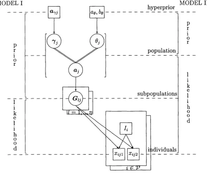
Figure 5 shows a directed acyclic graph (DAG) representing the Bayesian hierarchical model of Chapter 3.
When such a structure is used for diagnostic purposes, it is referred to as a probabilistic expert system [Cowell, Dawid, Lauritzen and Spiegelhalter, 1999]. The system provides a tool for specifying the joint distribution of all variables. For our purposes, the ‘irrelevancies’ summarised in the DAC describe conditional independence properties. For example, G can be seen to be independent of conditional upon a.
The additional labels on the DAC highlight the two possible statistical mod els.
Sections 4.1.1 and 4.1.2 consider these models in turn, before Section 4.2 considers inference about the match probability m/.
4.1.1 M o d e l I
Under model I, the likelihood is defined by the distribution of the data given the “param eter” G , the collection of subpopulation allele probability vectors (G{).
Calculation of the prior involves collapsing two levels to give a conditional dis tribution for G given the collection of hyperprior param eters ug, he) across the loci j = 1, . . . , M. Thus, the posterior distribution of our “param eter” G is
given by
f { G \ x a = I ) oc Pr(xa = & |G , / ) .7r(G |a^ , ug, he).
Under this model, the individuals are independent given the param eter, m ak ing the likelihood a straightforward expression (still considering m aternal and paternal bands to be distinguishable),
M
P^(%a — ^ a\ G ,I ) = %% %% G i-j{Xij\)G ^ iEa j=l
where a =
{
5}
U is the database expanded to include the suspect, and Xijb isMODEL II MODEL I
hyperprior
population
subpopulations
individuals
Figure 5: DAG for the case of complete information (at a fixed locus j), highlighting the two possible models. At this point we are assuming subpopulation identifiers (!{)
The subpopulation allele probabilities (Gi) are not independent given the hyperparam eters (a^j, a^, bg), but exchangeable. This makes the prior more difficult to derive:
7r(Glaj,a0,bd) = E[7r(G|a, ug, oo, 6g]
= J TT{G\a)7r{a\ary,a0,be)da (2 0)
= / • s s î i g ? g i i î r . w ' » »
_r(aj(+))
( = 1 J = J ^
a ^ j { k ) - l \ / 1 \ ae+rj-4
i S l S r a J
j l ^ w T î j
™
This expression for 7r{a\aj,ae, bg) is explained in more detail in Appendix B.
Equation (21) involves an integral across all {aj{k),j = =
l , . . . , r j ) , where aj(k) > 0. The form of this integral makes its calculation impossible using algebraic methods.
4 .1 .2 M od el II
Under model II the “param eter” is now a, and the prior is simply the prior of ttj {= ^ ^ 7 j) derived in Appendix B. This prior assumes, at each locus j ,
independence between the ancestral population allele probabilities 7^ and the
subpopulation differentiation parameters 9j:
~ Dirichlet(a.yj ( 1) , . . . , a^j(m^));
6j ~ Beta(u0,6g).
The likelihood involves collapsing the lower levels of the hierarchy to give the distribution of the data conditional upon the param eter a. Conditional upon
reason to distinguish individuals a priori, they are exchangeable. The likelihood is
Pr(Xa = = E[Pr(xa = ^a\G,a, I)\a, I]
=
/ g P r ( X a = Ç . l G , r ) . 7 r ( G | a ) d G
p M
— n n Giij{xiji)Gi-j{xij2)
i ea 7=1
T] m
n n i=i j=i
where nij{k) is the number of alleles of type k at locus j in subpopulation I
observed in the database. Given the subpopulation allele probability vectors
{Gij), these numbers (riij) have a multimomial distribution,
{nij{l),nij{2) , . . . , nij{rj)) ~ M ultinom ial(G (/l), G z /2) , . . . , Gij{rj)).
Thus, under model II, the posterior
f{a\Xa = oc Pr(xa = ^a|a)-7r ( a |a ^ ,a0,60)
for the chosen param eter is available up to a constant of proportionality.
4.2
Inference under th e two m odels
The subpopulation match probability
nil — — 3/1^ G 0 O!, Xq — ^aj P)
can be expressed as a posterior expectation of a function of either the model I param eters (Gij) (see (24) below) or the model II param eters (aj) (see (25) below),
where 4> represents the parameters under the chosen model.
Dawid [Dawid, 1986] notes th at if we have data Xq and wish to predict further observables X i it is often desirable to use a model in which, given pa rameters 9, X q and X i are independent. This means th a t the general predictive density of X i given Xq ,
f { x i \ x o ) =
j
f { x i \ e , Xo ) . f { 9 \ x o ) d 9simplifies to
I f ( x , \ e ) f ( 0 \ x o) d0 ,
the expectation of the density f { x i \ 9 ) with respect to the posterior distribution of 9 given the observed data Xq.
This property is achieved by model I, under which the culprit’s profile is independent of the observed data given the parameters (G;), implying that
Pr(Xi = x\ i G 'Pi, Xa — ^a)
= Pr(Xi = y|i e V,, G ) f { G \ i e P i , X a = U d G . (23)
In this instance, however, there is no great advantage provided by this property, as under model II the probability of the culprit’s profile given the param eter and d ata is reasonably straightforward to calculate (see (25) below).
As an aside, it is interesting to note th a t in their consideration of this prob lem, Foreman et al [Foreman, Evett and Smith, 1997] make a similar simplifica tion to th a t above, calculating the expectation of the probability of the culprit’s profile given their chosen parameters and the suspect’s profile only. However, as is described in Chapter 9, the model specification made by Foreman et al does not justify the assumption of independence between the culprit’s profile and the d ata conditional upon the parameters.
The match probability can be expressed as the following expectations;
mi = 'E[FT{Xi = y \ G , i e V i , I , X a = ^a)\l ^ P l , I , X a = ^a]
M
= = ( . ] (24)
where := .Gfj(r/j2) and
h(r, s) = 0 if r = s;
= 1 if r ^ s.
Also,
M
mi = E [ E [ n 2'‘'W'*'>^)G„fei).Gy(%2)|a, i e V,, J , Xa = &] j = l
|z G 7^1, I , X a — «Ca]
j=i k ( + ) + ’^ o (+ ))(^j(+ ) + ^ u (+ ) + 1)
N e ? , , / , % « = &] (25)
= E[mp^N G ' P/ , / , Xa = ^a], (26)
w V i P r P • - ( ° ji ^ n ) + ^ i j( % i ) ) K ( y j2) + n p - ( %2) + < * j ) wnere rrii . - llj= i / (a;(+)+n(;(+))K(+)+nu(+)+i)
0 if Vji f 2/j2
^ 1 if Vji = Vj2
Ideally we would calculate one or both of the expectations in equations (24) and (25) by integrating over the posterior distribution of the appropriate pa rameters.
The posterior distribution of G cannot be calculated even to proportionality. The posterior of a can be calculated to proportionality, but the integration re quired to evaluate the normalizing constant is not feasible using non-numerical methods. The desire for an inexpensive, easily applied m ethod would then dic ta te th at a reasonable approximation to the match probability mi be considered. This is where model I provides a more satisfactory answer, assuming th at we know the subpopulation labels (A) of each individual.
If the database a contains extensive d ata from subpopulation Vi, the expec tation of (24) can be approximated by a consistent estimate, for example
M ^ ^
= n (^j{y)Gij{yji)Gij{yj2), (27)
where Cj(y) = and Gij = representing the number of alleles of type k observed at locus j within individuals of subpopulation Vi in the database. It should be noted th a t (n/j) is only known if the individual subpopulation labels {Ii) are known.
While d ata from a large number of individuals will provide a consistent estimate of Gi which can be used to estimate the match probability, it is not generally possible to employ a similar approximation if the statistical model specified defines a as the parameter. As noted, a very large database will provide a large amount of information upon each set of subpopulation allele frequencies
G[. The collection of subpopulation frequencies at locus j [Gij] I = 1 , . . . ,ij) can be considered a random sample generated from the D iric h le t(a j(l),. . . ,% (rj)) distribution, with
1 - 9
— 'o' (7 7(1)5 • • ' 5 7 7(^7)),
where (6j) is a collection of subpopulation differentiation param eters and 7^ is
a vector of ‘ancestral population’ allele frequencies. This means th at, however extensive the database, the ‘sample size’ from which we may make estimates of
7 is limited to the number of subpopulations 77. Therefore, under model II a
consistent empirical estimator of a, which might be substituted in (25) instead of calculating the expectation, is not generally available.
Analagous to this situation is the example of a mint producing coins with bias varying about a mean, a. Tossing each of a sample of 77 coins a large number of
times will provide consistent estimates of the bias of each coin [Gi] I = 1, . . . , 77).
However even absolute knowledge of the bias of each of a small number of coins will not allow consistent estimation of the mean a of the process generating these biases.
A number of simplifications occur if the limit as the number
77 of subpopulations tends to infinity is considered. Roeder et al
[Roeder, Escobar, Kadane and Balazs, 1998] simplify the likelihood for the pop ulation parameters (7^) and {9j) by assuming th a t the probability of more than
der this assumption, all database individuals are independent given these pa rameters. The approach of Roeder et al is discussed further in Chapter 9,
4.3
Inference under unknown individual su b p op u lation
labels
The assumption th a t information is available identifying each individual’s sub population is generally unrealistic. Therefore, we can no longer condition upon
I in the match probability. Under model I,
= y |z G Xa ~
= E [P r(X i = y\G, I , i G Vi,Xa = G Vi.Xa = &]
= E [ n e V u Xa = &]. (28)
This is identical to equation (24), but excluding the conditioning upon I . Deriva tion of the likelihood of G now requires a summation over all possible I . It is assumed a priori th at subpopulation identifiers (7%) are independent across in dividuals. Also assuming th a t the subpopulation identifiers are independent of the subpopulation allele frequencies {Gi):
1{G) = Pr(x„ = Ç„|G)
= E[Pv(xa = U G , I ) \ G ) ]
= E
M
iea j=l
where k(1) is the prior probability th at an individual chosen at random is a
member of subpopulation Vi.
This is a sum over 77"“ terms, where ria is the number of individuals in the
across all possible combinations of subpopulation identifiers. If at all possible, this would be very computationally expensive, defeating the object of using such an estimator.
Under model II,
mi = P r(X i = y\ i e Vu Xa = (29)
= E[E[Pr(Xj = y | G , a , / , z G VuXa = € V u X a = («]
I* G V u X a — "Ca] (30) = E TT (%(^jl) + ^/j(^jl))(Q j(^j2) + ^lj{yj2) + <^j)
j = i (û j(+ ) + ^0'(+))(%■(+) + ^ b ( + ) + 1)
\ ^ ^ V u X a = ^a, (31)
(32)
where ôj indicates yji = yj2- Again, the data are no longer enough to evaluate n.
In the absence of an empirical estimator, it would appear necessary to eval uate one of the posterior expectations described in (28) and (30). As the inte gration required is impossible analytically, an alternative m ethod is required.
4.4
M arkov chain M onte Carlo
When direct solutions are unavailable due to the complex nature of the required integration, we resort to Markov chain Monte Carlo (MCMC) methods. These m ethods are discussed generally in Chapter 6, and specific schemes outlined in
Chapter 7.
It is im portant to relate ‘real world’ knowledge to the m athem atical problem at hand. There is a variety of possibilities regarding the state of our knowledge of subpopulation identifiers and related quantities such as subpopulation propor tions a . Chapter 8 seeks to describe the effect of varying this knowledge upon
5
M easures o f subpopulation differentiation
Throughout the extensive literature concerning population substructure, param eters which it is claimed quantify the differentiation between subpopulations are defined by a number of authors.
Indeed the param eter 0 = {9j\j = 1 , . . . , M) of the model defined in Chapter 3 can be seen as a subpopulation differentiation parameter. If reasonable models are to be developed, it is very useful to be able to relate the param eters of such models to meaningful ‘real world’ quantities. W hat does 0 really mean? Which, if any, of the population genetics differentiation parameters is it equivalent to? These are interesting and im portant questions which are not always answered satisfactorily.
As will be seen in this chapter, the degree of difference between param eters which have in some instances been regarded as equivalent is as great as th a t between sample and population variances.
To dem onstrate this, the subpopulation differentiation param eters of Nei [Nei,1987] and Weir and Cockerham [Weir and Cockerham, 1984] are compared in the context of the hierarchical model described in Chapter 3. Papers employ ing models of population substructure often make no distinction between the two, classing them as equivalent.
To simplify m atters, the two allele (0 and 1) single binary locus case is considered here, where P r(%*6 = 1|G) = Gi for each band (6 = 1,2) within each
individual i in subpopulation Vi.
We define n (= « (/);/ = 1 , . . . , 77) as the collection of prior probabilities of a
randomly selected individual i being in subpopulation Vi'. K,{1) = Fr{Ii = I),
5.1
N ei
Nei considers the fixation index F to be a function of the param eters defining the allele probabilities {Gi) of the 77 actual subpopulations. Using only these
present generation parameters, no assumption is required about pedigrees of individuals, selection and migration in the past.
We define
9 = /=!
the average of the subpopulation allele ‘1’ probabilities, weighted by k.
If the current population is in Hardy-Weinberg equilibrium we have the case where 77 = 1 and g = Gi'.
P r(X , = (0 ,0 )|^,G ) = ( l - g f - ,
P r(X i = (0, l ) | p , G) = 2 g { l - g ) ;
P r(X , = ( l,l ) |p ,G ) = g^.
Following the thinking of Wright [Wright, 1951], any departure from these Hardy-Weinberg probabilities can be measured by the fixation index F so th a t
P r(X , = (0 ,0 )|^ ,G ) = { l - F ) { l - g f F F ( l - g ) - (33)
P r(X , = (0 ,l)|p ,G ) = 2 ( l - F ) g { l - g ) ; (34)
P r(X i = (l , l )| ff , G) = ( 1 - F ) g ^ + Fg. (35)
There are a number of possible causes of departure from Hardy-Weinberg pro portions, including inbreeding, assortative m ating and selection. At this point, however, we consider only the effect upon overall proportions of a population be ing split into 77 randomly mating subpopulations. The overall pair probabilities
are then given by
V
/=!
— (1 ~ ^)^ + ^ ( 0 [(1 ~ ^ i ) “ (1 “ g)Ÿ
1=1
P r(X , = ( 0 ,l) |s ,G ) = 2 Y ^ K { l ) G , ( \ - G i ) - = 2 g { l - g ) - 2 a \ (37)
/ = 1
P r(X i = ( l , l ) |5, G) = j ^K ( l )G ] = g'^ + a'^-, (38)
Z=1
where <7^ = YJi=i the ‘sample’ variance of the gene ‘1’ proportion
across subpopulations. The homozygotic frequencies are increased above the Hardy-Weinberg level by an amount cr^ with an appropriate reduction in the heterozygotic frequency. Comparison of equations (33)-(35) to (36)-(38) shows th a t the fixation index in the case of 2 alleles is then given by
F =
g { ^ - 9)'
5.2
W eir and Cockerham
In terms of the hierarchical model, Weir and Cockerham work at the level above Nei. Weir and Cockerham define a coancestry coefficient 6 th a t does not depend upon the number of subpopulations observed and governs the level of variability of allele probability (Gi) across subpopulations. It is a param eter related to the ancestral population from which the currently observed subpopulations have developed. To Weir and Cockerham, the observed subpopulations are just a sample of those th at could have evolved from the ancestral population under similar conditions. This is directly comparable to the hierarchical model in which the 77 subpopulations are a sample generated given the param eters of the
level above.
The subpopulations (P/; I = 1, . . . ,77) are assumed to have descended sepa
rately from the single ancestral population.
Random m ating is assumed within subpopulations, and we define 7 as the
mean of the process generating subpopulation probabilities (Q ), i.e.
E[G/|7] = 7,
independently for all 1. Weir and Cockerham then define their subpopulation differentiation param eter 9 by
Referring to the DAG of Figure 5, the probabilities {Gi) are defined at the level of the subpopulations. We assume th at these probabilities are generated with a mean 7 and variance V. The im portant point here is th a t 7 and V are
param eters at the level above (Gi) in the hierarchy. In the previous section, g
and are defined at the same level as (G/).
Pr(%, = ( l , l ) | 7 , n = E[Pr(X, = ( l , l ) | 7 , R )
= E[Pr(%, = ( l , l ) | G , 7 , n
=
E[/{(/)G^|7,y)
= + = ^ + f (40)
1=1
By comparison of equations (39) and (40), we see th a t 6 = a measure of subpopulation differentiation at the level above Nei’s param eter F.
5.3
H ow are th e m easures o f su b p op u lation differentia
tio n related?
Firstly it is interesting to compare directly the definitions of Nei’s param eter F,
and Weir and Cockerham’s 6.
6 =
7(1 - 7) ’
Presented in this way, one can see the justification behind the earlier statem ent th a t the comparison is similar to th at between a sample variance and a pop ulation variance. The differences in definition between g = i^{l)Gi and
7 = ElGil'y] should also be noted.
It is also helpful to consider the expectation of the ‘sample variance’ (= — p)^), given 7 and the prior variance V and 7.
E [a^|y,7] = E [ ' £ < l ) { G , - g Y \ V , j ] I
= e E k ( ; ) g ? - s ^ | v , 7 ]
= E «(OEfG^lF,7] - V ax(s|F,7) - E [g |y ,7]^
l
= V ar(g |y ,7) + E[g\V,7]' - V a r ( ^ i^{l)G,\V,7) - Ÿ
l = V + - Y ^ K { i f v
l I
E[(7^|y,7] = y E 4 0 ( i - 4 0 )
I
In the special case where k,{1) = ^ for / = 1, . . . , 77, this simplifies to 9|TT -1 ^ “ 1
meaning th at
E [ F s ( l -5)10,7] = ^ 0 7(1 - 7), (41)
Equation (41) clarifies the role of the subpopulation differentiation parameters,