Sliding mode \({H {\infty}}\) synchronization for complex dynamical network systems with Markovian jump parameters and time varying delays

(1)

R E S E A R C H

Open Access

Sliding-mode

H

_∞

synchronization for

complex dynamical network systems with

Markovian jump parameters and

time-varying delays

Nannan Ma

1*

_{, Zhibin Liu}

1

_{and Lin Chen}

1

*_{Correspondence:} [email protected] 1_{School of Science, Southwest} Petroleum University, Chengdu, China

Abstract

This paper is devoted to the investigation of the sliding-mode controller design problem for a class of complex dynamical network systems with Markovian jump parameters and time-varying delays. On the basis of an appropriate

Lyapunov–Krasovskii functional, a set of new suﬃcient conditions is developed which not only guarantee the stochastic stability of the sliding-mode dynamics, but also satisfy theH∞performance. Next, an integral sliding surface is designed to guarantee that the closed-loop error system reach the designed sliding surface in a ﬁnite time. Finally, an example is given to illustrate the validity of the obtained theoretical results.

Keywords: Complex dynamical networks; Sliding-mode control; Markovian jump parameters;H_∞performance

1 Introduction

In recent years, increasing attention has been drawn to the problem of complex networks due to their potential applications in many real-world systems, such as biological systems, chemical systems, social systems and technological systems. In particular, the synchro-nization phenomena in complex dynamical networks system have attracted rapidly in-creasing interests, which mean that all nodes can reach a common state. Several famous network models, such as the scale-free model [1] and the small-word model [2,3], which accurately characterize some important natural structures, have been researched. Com-plex dynamical network are prominent in describing the sophisticated collaborative dy-namics in many ﬁelds of science and engineering [4–6].

The feature of time delay exists extensively in many real-world systems. It is well known that the existence of time delay in a network can make system instable and degrade its per-formance. In recent decades, considerable attention has been devoted to the time-delay systems due to their extensive applications in practical systems including circuit theory, neural network [7–10] and complex dynamical networks system [11–16] etc. Thus, syn-chronization for complex dynamical networks with time delays in the dynamical nodes and coupling has become a key and signiﬁcant topic. Some researchers have proposed some results in this area. In [11], the author proposed pinning control scheme to achieve

(2)

synchronization for singular complex networks with mixed time delays. Based on impul-sive control method, the authors in [12,13] studied projective synchronization between general complex networks with coupling time-varying delay and multiple time-varying de-lays [14], respectively. Based on sampled-data control [15], the authors proposed a method with ﬁnite-timeH∞ synchronization in Markovian jump complex networks with time-varying delays. Based on pinning impulsive control [17], the problem of exponential syn-chronization of Lur’e complex dynamical network with delayed coupling was studied.

The dynamical behaviors of all nodes in complex dynamical networks are not always the same. Thus, many authors have studied the characteristics of all nodes in CDNs with the help of digital controllers, such as pinning control [18–21], sampled-data control [22,23], impulsive control [24–26] and sliding control [27–30] and so on. Under an important pin-ning control approach, by a minimum number of controllers, the system can reached the predetermined goal. Under a sampled-data controller, the states of the control systems at sampling instants are adjusted continuously by using zero-order holder. Under an im-pulsive controller, states of the control systems are adjusted at discrete-time sampling in-stants. Under sliding control, in the design of the sliding surface, a set of speciﬁed matrices are employed to establish the connections among sliding surface corresponding to every mode. No matter what control strategy is adopted, the ultimate goal is to make the system stable and achieve our intended results. In this paper, the goal is to select suitable slid-ing control to synchronize complex networks with Markovian jump parameters and time delays.

The sliding-mode control methods were initiated in the former Soviet Union about 40 years ago, and since then the sliding-mode control methodology has been receiving much more attention within the last two decades. Sliding-mode control is widely adopted in lots of complex and engineering systems, including time delays [31–33] stochastic sys-tems [34,35], singular systems [36–38], Markovian jumping systems [39–41], and fuzzy systems [42–44]. As is well known, system performance may be degraded by the aﬀection of the presence of nonlinearities and external disturbances. In [32], a sliding-mode ap-proach is proposed for the exponentialH∞synchronization problem of a class of master–

slave time-delay systems with both discrete and distributed time delays. In [34], the au-thors were concerned with event-triggered sliding-mode control for an uncertain stochas-tic system subject to limited communication capacity. In [38], this paper is concerned with non-fragile sliding-mode control of discrete singular systems with external distur-bance. In [41], the authors considered sliding-mode control design for singular stochastic Markovian jump systems with uncertainties. The main advantage of the sliding mode is low sensitivity to plant parameter variation and disturbance, which eliminate the necessity of exact modeling.

Markovian jump systems including time-evolving and event-driven mechanisms have the advantage of better representing physical systems with random changes in both struc-ture and parameters. Much recent attention has been paid to the investigation of these systems. When complex dynamical networks systems experience abrupt changes in their structure, it is natural to model them by Markovian jump complex networks systems. A great deal of literature has been published to study the Markovian jump complex net-works systems; see [11,14,15,19,23,28] for instance.

(3)

time-varying delays coupling in the dynamical nodes. So it is challenging to solve this synchro-nization problem for complex dynamical networks. Motivated by the aforementioned dis-cussion, this paper aims to study theH∞synchronization of complex dynamical network system. To achieve theH∞synchronization of complex dynamical networks with

Marko-vian jump parameter, the integral sliding surface is designed, and a novel sliding-mode controllers is proposed. The main contributions of this article are summarized as follows: (1) This paper extends previous work on the synchronization problem for complex dy-namical network systems with Markovian jump parameters and time-varying delays and derives some new theoretical results. (2) An appropriate integral sliding-mode surface is constructed such that the reduced-order equivalent sliding motion can adjust the eﬀect of the chattering phenomenon. (3) Using a Lyapunov–Krasovskii functional and a sliding-mode controller, we establish new suﬃcient conditions in terms of LMIs to ensure the stochastic stability and theH∞performance condition.

Notation Rn_{denotes the}_n_{dimensional Euclidean space;}_Rm×n_{represents the set of all}

m×nreal matrices. For a real asymmetric matrixXandY, the notationX≥Y (respec-tively,X>Y ) meansX–Yis semi-positive deﬁnite (respectively, positive deﬁnite). The superscriptTdenotes matrix transposition. Moreover, in symmetric block matrices,∗is used as an ellipsis for the terms that are introduced by asymmetry anddiag{· · · }denotes a block-diagonal matrix. The notationA⊗Bstands for the Kronecker product of matri-cesAandB. · stands for the Euclidean vector norm.E stands for the mathematical expectation. If not explicitly stated, matrices are assumed to have compatible dimensions.

2 System description and preliminary lemma

Let{r(t) (t≥0)}be a right-continuous Markovian chain on the probability space (Ω,F,

{Ft}t≥0,P) taking a value in the ﬁnite spaceS={1, 2, . . . ,m}, with generatorΠ={πij}m×m

(i,j∈S) given as follows:

Pr(rt+t=j|rt=i) = ⎧ ⎨ ⎩

πijt+o(t), i=j,

1 +πijt+o(t), i=j,

wheret> 0,limt→0(ot/t) = 0, andπijis the transition rate from modeito modej

satisfyingπij≥0 fori=jwithπij= –

m

j=1j=iπij(i,j∈S).

The following complex dynamical network systems ofNidentical nodes is considered, in which each node consists of ann-dimensional dynamical subsystem with Markovian jump parameter and time delay:

⎧ ⎪ ⎪ ⎨ ⎪ ⎪ ⎩ ˙

xk(t) =A(r(t))xk(t) +C(r(t))f(xk(t)) +σ1

N

j=1gkjΓ1(r(t))xj(t)

+σ2

N

j=1gkjΓ2(r(t))xj(t–τ(t)) +D(r(t))wk(t) +B(r(t))uk(t),

zk(t) =E(r(t))xk(t), k= 1, 2, . . . ,N,

(1)

where xk(t) = (xk1,xk2, . . . ,xkn)T ∈Rnrepresents the state vector of thekth node of the

complex dynamical system;uk(t) denote the control input andwk(t) is the disturbance;

f(xk(t)) is for vector-valued nonlinear functions;A(r(t)),C(r(t)),D(r(t)) andB(r(t)) are

(4)

inner coupling matrix of the complex networks;σ1 andσ2> 0 denote the non-delayed and delayed coupling strengths.G= (gkj)N×N is the out-coupling matrix representing the

topological structure of the complex networks, in whichgkjis deﬁned as follows: if there

exists a connection between nodekand nodej(k=j), thengkj=gjk= 1, otherwise,gkj=

gjk = 0 (k=j). The row sums of Gare zero, that is, N

j=1gkj= –gkk,k= 1, 2, . . . ,N. The

bounded functionτ(t) represents unknown discrete-time delays of the system. The time delayτ(t) is assumed to satisfy the condition as follows:

0≤τ(t)≤τ, 0≤ ˙τ(t)≤ ¯τ, (2)

whereτ andτ¯are given nonnegative constants.

Assumption 2.1 For allx,y∈Rn_{, the nonlinear function}_f₍_·_{) is continuous and assumed}

to satisfy the following sector-bounded nonlinearity condition:

f(x) –f(y) –U1(x–y)

T

f(x) –f(y) –U2(x–y)

≤0, (3)

whereU1andU2∈Rn×nare known constant matrices withU2–U1> 0. For presentation simplicity and without loss of generality, it is assumed thatf(0) = 0.

Deﬁnition 2.1([41]) The complex dynamical network systems (1) is said to be stochas-tically stable, if anye(0)∈Rn_and_r

0∈Sthere exists a scalarM˜(e(0),r0) > 0 such that

lim t→∞E

t

0

eTs,e(0),r0

es,e(0),r0

≤ ˜Me(0),r0

,

wheree(t,e(0),r0) denotes the solution under the initial conditione(0) andr0. Andek(t) =

xk(t) –s(t) is the synchronization error of the complex dynamical network system, and

s(t)∈Rncan be an equilibrium point, or a (quasi-)periodic orbit, or an orbit of a chaotic attractor, which satisﬁes˙s(t) =A(r(t))s(t) +C(r(t))f(s(t)).

Deﬁnition 2.2([32]) TheH∞performance measure of the systems (1) is deﬁned as

J∞=E

∞

0

ze(t)Tze(t) –γ2wT(t)w(t)dt

,

where the positive scalarγ is given.

Lemma 2.1(Jensen’s inequality) For a positive matrix M,scalar hU>hL> 0the following

integrations are well deﬁned: (1) –(hU–hL)

t–hL

t–hUx

T₍_s₎_Mx₍_s₎_ds_≤_–(t–hL

t–hUx

T₍_s₎_ds₎_M₍t–hL

t–hUx

T₍_s₎_ds₎_,

(2) –(h2U–h2L

2 )

t–hL

t–hU

t

s xT(u)Mx(u)du ds≤–( t–hL

t–hU

t

sxT(u)du ds)M( t–hL

t–hU

t

sx(u)du ds).

Lemma 2.2([11]) If for any constant matrix R∈Rm×m_,_R₌_RT _{> 0,}_scalar_γ _{> 0}_{and a}

vector functionφ: [0,γ]→Rmsuch that the integrations concerned are well deﬁned,the following inequality holds:

–γ

t

t–γ ˙

φT(s)Rφ˙(s)ds≤

φ(t)

φ(t–γ)

T

–R R

∗ –R

φ(t)

φ(t–γ)

(5)

Lemma 2.3([45]) Let⊗denote the Kronecker product.A,B,C and D are matrices with appropriate dimensions.The following properties hold:

(1) (cA)⊗B=A⊗(cB),for any constantc, (2) (A+B)⊗C=A⊗C+B⊗C,

(3) (A⊗B)(C⊗D) = (AC)⊗(BD), (4) (A⊗B)T=AT⊗BT,

(5) (A⊗B)–1_{= (}_A–1_⊗_B–1₎_.

For the sake of simplicity, when r(t) =i, we denoteAi, Ci, Bi, Di, Γ1i, Γ2i asA(r(t)),

C(r(t))B(r(t)),D(r(t)),Γ1(r(t)),Γ2(r(t)). Lete(t) =x(t) –s(t) be the synchronization error of system from the initial moder0. Then the error dynamical, namely, the synchronization error system can be expressed by

⎧ ⎪ ⎪ ⎨ ⎪ ⎪ ⎩ ˙

ek(t) =Aiek(t) +Cig(ek(t)) +σ1Nj=1gkjΓ1iej(t) +σ2Nj=1gkjΓ2iej(t–d(t))

+Biuk(t) +Diwk(t),

zk(t) =Eiek(t), k= 1, 2, . . . ,N,

(4)

whereg(ek(t)) =f(xk(t)) –f(sk(t)).

Now, the original synchronization problem can be replace by the equivalent problem of the stability the system (4) by a suitable choice of the sliding-mode control. In the fol-lowing, the sliding-mode controller will be designed using variable structure control and sliding-mode control methods [46]. Let us introduce the sliding surface as

Sk(t,i) =Viek(t) –Vi t

0

(Ai–BiKi)ek(s) +σ1

N

j=1

gkjΓ1iek(s)

+σ2

N

j=1 gkjΓ2iek

s–d(s)

ds. (5)

Vi∈Rm×n,Ki∈Rr×nare real matrices to be designed.Viis designed such thatViBiis

non-singular. It is clear thatS˙k(t,i) = 0 is a necessary condition for the state trajectory to stay

on the switching surfaceSk(t,i) = 0. Therefore, byS˙k(t,i) = 0 and (4), we get

0 =ViBiKiek(t) +ViCig

ek(t)

+ViBiuk+ViDiwk(t). (6)

Solving Eq. (6) foruk(t)

ukeq(t) = –Kiek(t) –VˆiCig

ek(t)

–VˆiDiwk(t), (7)

whereVˆi= (ViBi)–1Vi.

Substituting (7) into (4), the error dynamics with sliding mode is given as follows:

⎧ ⎪ ⎪ ⎨ ⎪ ⎪ ⎩ ˙

ek(t) = (Ai–BiKi)ek(t) + (Ci–BiVˆiCi)g(ek(t))

+σ1Nj=1gkjΓ1iej(t) +σ2Nj=1gkjΓ2iej(t–d(t)) + (I–BiVˆi)Diwk(t),

zk(t) =Eiek(t).

(6)

Or equivalently

The problem to be addressed in this paper is formulated as follows: given the complex dynamical network system (1) with Markovian jump parameters and time delays, ﬁnding a mode-dependent sliding mode stochastically stable andH∞synchronization controlu(t) with anyr(t) =i∈Sfor the error system (4) is stochastically stable and satisﬁes anH∞

norm boundγ, i.e.J∞< 0.

3 Main results

The purpose of this section is to solve the problem ofH∞synchronization. More

speciﬁ-cally, we will establish LMI conditions to check whether the sliding-mode dynamics have ideal properties, such as being stochastically stable andH∞synchronization. The relevant

conclusion of the stability analysis is provided in the following theorem.

3.1 Stability analysis

Theorem 3.1 Let the matrices Vi,Ki(i= 1, 2, . . . ,N)withdet(ViBi)= 0be given.The

com-plex dynamical network system(1)with Markovian jump parameter is stochastically stable and shows H∞synchronization in the sense of Deﬁnition2.1and Deﬁnition2.2,if there

(7)

Φ56= –

Proof Design the following positive deﬁnition functional for the system:

Ve(t),i,t=V1

By the deﬁnition of the inﬁnitesimal operatorLof the stochastic Lyapunov–Krasovskii functional in [47], we obtain

LVe(t),i,t= lim

(8)

+ 2

According to Lemma2.1and Lemma2.2, we have

–

For any matricesΛ1andΛ2with appropriate dimensions, the following equations hold:

(9)

×–e˙(t) +IN⊗(Ai–BiKi)

e(t) +IN⊗(Ci–BiVˆiCi)

ge(t)

+σ1(G⊗Γ1i)e(t) +σ2(G⊗Γ2i)e

t–τ(t)+IN⊗(Di–BiVˆiDi)

w(t). (22)

It can be deduced from Assumption2.1that, for the matricesU1andU2, the following inequalities hold:

y(t) =ε

e(t) g(e(t))

T

¯

R S¯

∗ I

e(t) g(e(t))

≤0, (23)

where

¯

R=(IN⊗U1)

T₍_I

N⊗U2) + (IN⊗U2)(IN⊗U1)T

2 ,

¯

S=(IN⊗U2)

T_{+ (}_I

N⊗U1)T

2 .

On the other hand, for a prescribedγ> 0, under zero initial condition,J∞can be

rewrit-ten as

J∞≤E

∞

0

e–2αtzT(t)z(t) –γ2wT(t)w(t)dt+Ve(t),i,t|t→∞

–Ve(t),i,t|t=0

≤E ∞

0

e–2αt_zT₍_t₎_z₍_t_{) –}_γ2_wT₍_t₎_w₍_t₎₊_L_V_e₍_t_),_i_,_t_dt

. (24)

From the obtained derivation terms in Eqs. (16)–(21) and adding Eqs. (22)–(23) into (24)

J∞≤E

∞

0

ξT(t)Φiξ(t)dt

, (25)

where

ξ(t) =

eT₍_t₎ _eT₍_t_–_τ₎ _eT₍_t_–_τ₍_t₎₎₍t

t–τe(s)ds) T

gT₍_e₍_t₎₎ _e_˙T₍_t₎ _wT₍_t₎T_.

According to the condition (10) in Theorem3.1, it means that the conditionJ∞< 0 is

satisﬁed. Moreover,J∞< 0 forw(t) = 0 impliesE{LV(e(t),i,t)}< 0. Then we have

ELVe(t),i,t< –a1E

eT(t)e(t), (26)

wherea1=min{λmin(–Φi),i∈S}, thena1> 0. By Dynkin’s formula, we have

E t

0

eT(s)e(s)ds

≤a–1₁ Ve(0),r0, 0 (27)

and

lim t→∞E

t

0

eT(s)e(s)ds

≤a–1₁ Ve(0),r0, 0

(10)

Then from Deﬁnition2.1, the sliding-mode dynamical system (9) is stochastically stable.

This completes the proof.

Remark1 It should be pointed out that Theorem3.1provided a suﬃcient condition of stability for the sliding-mode complex dynamical network systems (9). But the parameter matrix is not given so we cannot apply the LMI toolbox of Matlab to solve them. According to Theorem3.1and the Schur complement, the strict LMI conditions will be given in the next theorem.

Theorem 3.2 Under Assumption2.1,a synchronization law given in the form of Eq. (9) exists such that the Markovian jump synchronization error system(9)with time-varying delays is stochastically stable and an H∞ performance levelγ > 0in the sense of Defini-tion2.1and Definition2.2,if there exist some matrices Yi,Vˆiand positive definite matrices

(11)

Σ67=Λ˜T2

IN⊗(Di–BiVˆiDi)

,

Σ18=e–ατ(IN⊗Mi)(IN⊗E)T,

Σ19=

√

πi1(IN⊗Mi),√πi2(IN⊗Mi), . . . ,√πis(IN⊗Mi)

,

Σ99=diag

–(IN⊗M1), –(IN⊗M2), . . . , –(IN⊗Ms)

.

Proof Using the following diagonal matrix:

diag(IN⊗Pi)–1, (IN⊗Pi)–1, (IN⊗Pi)–1, (IN⊗Pi)–1,I, (IN⊗Pi)–1,I

and its transpose, to pre-multiplying and post-multiplying (11), whereMi=Pi–1, applying

Schur complements and Lemma2.3and consideringKiMi=Yi, we can get (29). Thereby

the proof of the theorem is completed.

3.2 Sliding-model control design

The objective now is to study the reachability. In this section, an appropriate control law will be constructed to drive the trajectories of the system (1) into the designed sliding surfaceSk(t,i) = 0 withSk(t,i) deﬁned in (6) in ﬁnite time and maintain them on the surface

afterwards.

Theorem 3.3 Suppose that the sliding function is given in(6)where Ki and Mi satisfy

(29)–(30).Then the trajectories of the error dynamic system(9)can be driven onto the slid-ing surface Sk(t,i) = 0in ﬁnite time and then maintain the sliding motion if the control is

designed as follows:

uk(t) = –Kiek(t) –

δki+ B–1i Cig

ek(t) +ρi wk(t) sign

BT_iV_iTS(k,i), (31)

whereρi:=maxi∈S(λmax(DiDTi))0.5.

Proof Choose the following Lyapunov function:

WSk(t,i)

=1 2S

T

k(t,i)Sk(t,i). (32)

Calculating the time derivative of the sliding-mode surfaceSk(t,i) along the trajectory

of (4), we obtain

˙

WSk(t,i)

=ST_k(t,i)S˙k(t,i)

=ST_k(t,i)Vi !

˙

ek(t) –

(Ai–BiKi)ek(t) +σ1

N

j=1

gkjΓ1iej(t)

+σ1

N

j=1 gkjΓ2iej

t–d(t)

"

=ST k(t,i)Vi

BiKiek(t) +Cig

ek(t)

+Biuk(t) +Diwk(t)

=ST_k(t,i)ViBi

uk(t) +Kiek(t) +B–1i Cig

ek(t)

(12)

≤ST_k(t,i)ViBi

uk(t) +Kiek(t)

+ B–1_i Cig

ek(t) +ρi wk(t) BTiViTSk(t,i) . (33)

Substituting (31) into (33) implies that

˙

WSk(t,i)

≤–δki BTiViTSk(t,i) ≤– √

2δkiλmin(ViBi)W0.5

Sk(t,i)

. (34)

Then, lettingSk(t0= 0,r0) =Sk0and integrating from 0→t, one obtains

EWSk(t,i)

|Sk0,r0

0.5

≤–

√

2

2 δkiλmin(ViBi)t+W 0.5₍_S

k0,r0). (35)

The left-hand side of (35) is nonnegative; we can judge thatW(Sk(t,i)) reaches zero in

ﬁnite time for each modei∈S={1, 2, . . . ,m}, and the ﬁnite timet∗is estimated by

t∗≤

√

2W(Sk0,r0)

δkiλmin(ViBi)

. (36)

Therefore, it is shown from (36) that the system trajectories can be driven onto the pre-deﬁned sliding surface in ﬁnite time. In other words, the sliding-mode surfaceSk(t,i) must

be reachable.

Remark2 In order to eliminate the chattering caused bysign(BT_i V_iTS(k,i)), a boundary layer is introduced around each switch surface by replacesign(BT

iViTS(k,i)) in (31) by

sat-uration function. Hence, the control law (31) can be expressed as

uk(t) = –Kiek(t) –

δki+ B–1i Cig

ek(t) +ρi wk(t) sat

BT

iViTS(k,i)

κ

. (37)

Thejth element ofsat(BT_i V_iTS(k,i)/κ) is described as

sat _[_VT

i BTiSk(t,i)]_j

κj

=

⎧ ⎨ ⎩

[sign(V_iTBT_iSk(t,i))]j, if [ViTBTiSk(t,i)]j>κj,

[V_iTBT_iSk(t,i)]_j

κj , otherwise,

(38)

wherej= 1, 2, . . . ,m,κjis a measure of the boundary layer thickness around thejth

switch-ing surface.

4 Example

In this section, an example is provided to demonstrate that the proposed method is eﬀec-tive.

Example1 Consider complex dynamical networks systems (1) with three nodes and mode

S={1, 2}. The relevant parameters are given as follows. Mode 1:

A1=

–0.1 0.1

0 –0.2

, B1=

–1 0

0 –1

, C1=

1 0

0 1

(13)

D1= And the outer coupling matrix is given as

G=

The LMIs (29) in Theorem3.2are solved by Matlab LMI toolbox, and obtainedγ = 8.4702e+04.

2.6572 0.0178 0.0007 0.0005 0.0007 –0.0067

0.0178 2.6863 –0.0004 0.0066 –0.0015 0.0091

0.0007 –0.0004 2.6572 0.0197 0.0010 –0.0024

0.0005 0.0066 0.0197 2.6325 0.0009 0.0272

0.0007 –0.0015 0.0010 0.0009 2.5636 –0.0356

–0.0067 0.0091 –0.0024 0.0272 –0.0356 2.6089

⎤

38.0472 –1.1333 –0.0541 –0.4213 –0.1619 0.4567

0.9337 72.0648 –0.3623 6.1533 –2.7151 –10.2644

0.1775 0.3276 38.0115 –1.0913 0.1921 0.3917

0.3648 –4.4085 1.0863 68.9744 –0.6696 4.2949

0.4862 2.7744 0.0387 0.6443 37.6727 –2.6762

–0.3795 11.3680 –0.3935 –1.8270 2.2792 86.5689

(14)

˜

75.9386 –2.2126 –0.0752 –0.8326 –0.0613 0.3964

1.7490 143.3691 0.1992 10.0380 –5.0827 –20.6567

0.3153 –0.2654 75.8670 –1.4096 0.5290 0.9310

0.7231 –6.7185 1.3070 137.5655 –1.1323 7.1219

0.7064 5.1990 –0.0751 1.0765 75.1961 –5.2959

–0.2254 22.8512 –0.9253 –2.5126 4.6910 172.5156

⎤

3.8856 0.0424 –0.0020 0.0017 –0.0001 –0.0156

0.0424 3.9816 –0.0011 0.0059 –0.0041 0.0181

–0.0020 –0.0011 3.8928 0.0451 –0.0080 –0.0050

0.0017 0.0059 0.0451 3.8696 0.0012 0.0447

–0.0001 –0.0041 –0.0080 0.0012 3.8835 –0.0819

–0.0156 0.0181 –0.0050 0.0447 –0.0819 3.8253

⎤

2.8470 0.0225 0.0009 0.0005 0.0009 0.0083

0.0225 2.8972 –0.0006 0.0086 –0.0020 0.0118

0.0009 –0.0006 2.8469 0.0247 0.0013 –0.0030

0.0005 0.0087 0.0247 2.8285 0.0011 0.0349

0.0009 –0.0020 0.0013 0.0011 2.8424 –0.0443

–0.0083 0.0118 –0.0030 0.0349 –0.0443 2.8071

⎤

The gain matricesK1,K2can be obtained by simple calculation,

K1=Y1M–11 =

Moreover, by (5), settingVi=Vˆithe switching surface function can be computed as

Sk(t, 1) =V1ek(t) –V1

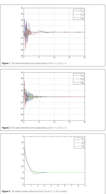
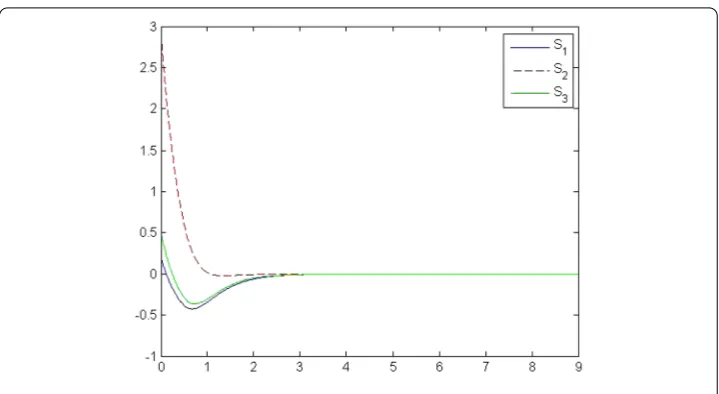
The simulation results are presented in Figs.1–4. It can be seen from Figs.1and2that the synchronization error converges to zero in mode 1 and mode 2, respectively. Figures3

and4demonstrate the sliding-mode surface function in mode 1 and mode 2, respectively.

5 Conclusion

(15)

Figure 1The state estimation error trajectorieseki(t) (k= 1, 2, 3) (i= 1)

Figure 2The state estimation error trajectorieseki(t) (k= 1, 2, 3) (i= 2)

(16)

Figure 4The sliding-mode surface functionSk(t) (k= 1, 2, 3) in mode 2

and time-varying delays. A novel integral sliding-mode controller was proposed. On the basis of Lyapunov stability theory, it has been shown that the Markovian jump complex dynamical network systems via sliding-mode control can be guaranteed to show synchro-nization and satisfyH∞ performance. An example was given to shown the eﬀectiveness

of the obtained methods.

It would be interesting to extend the results obtained to multiple complex dynamical networks with multiple coupling delays. This topic will be considered in future work.

Funding

This paper was supported in part by the Applied Fundamental Research (Major frontier projects) of Sichuan Province of China (Grant No. 2016JC0314). The authors would like to thank the editor and anonymous reviewers for their many helpful comments and suggestions to improve the quality of this paper.

Competing interests

The authors declare that they have no competing interests.

Authors’ contributions

All authors read and approved the ﬁnal manuscript.

Publisher’s Note

Springer Nature remains neutral with regard to jurisdictional claims in published maps and institutional aﬃliations.

Received: 6 November 2018 Accepted: 22 January 2019

References

1. Barabasi, A.L., Albert, R., Jeong, H.: Scale-free characteristics of random networks: the topology of the world wide web. Physica A281(1), 69–77 (2000)

2. Watts, D.J., Strogatz, S.H.: Collective dynamics of ‘small-world’ networks. Nature393, 440–442 (1988) 3. Barbasi, A.L., Albert, R.: Emergence of scaling in random networks. Science286, 509–512 (1999) 4. Albert, R., Jeong, H., Barabsi, A.L.: Diameter of the world wide web. Nature401, 130–131 (1999) 5. Strogatz, S.H.: Exploring complex network. Nature410, 268–276 (2001)

6. Wang, X.F., Chen, G.R.: Synchronization in scale-free dynamical networks: robustness and fragility. IEEE Trans. Circuits Syst.149, 54–56 (2002)

7. Peng, X., Wu, H.Q., Song, K., Shi, J.X.: Global synchronization in ﬁnite time for fractional-order neural networks with discontinuous activations and time delays. Neural Netw.94, 46–54 (2017)

8. Liu, M., Wu, H.Q.: Stochastic ﬁnite-time synchronization for discontinuous semi-Markovian switching neural networks with time delays and noise disturbance. Neurocomputing310, 246–264 (2018)

9. Peng, X., Wu, H.Q., Cao, J.D.: Global nonfragile synchronization in ﬁnite time for fractional-order discontinuous neural networks with nonlinear growth activations. IEEE Trans. Neural Netw. Learn. Syst. (2018, in press).

(17)

10. Zhao, W., Wu, H.Q.: Fixed-time synchronization of semi-Markovian jumping neural networks with time-varying delays. Adv. Diﬀer. Equ.2018, 213 (2018)

11. Ma, Y.C., Ma, N.N., Chen, L.: Synchronization criteria for singular complex networks with Markovian jump and time-varying delays via pinning control. Nonlinear Anal. Hybrid Syst.28, 85–99 (2018)

12. Zheng, S.: Projective synchronization in a driven-response dynamical network with coupling time-varying delays. Nonlinear Dyn.63(3), 1429–1438 (2012)

13. Zheng, S.: Projective synchronization analysis of drive-response coupled dynamical network with multiple time-varying delays via impulsive control. Abstr. Appl. Anal.2014, Article ID581971 (2014)

14. Ma, Y.C., Zheng, Y.Q.: Synchronization of continuous-time Markovian jumping singular complex networks with mixed mode-dependent time delays. Neurocomputing156, 52–59 (2015)

15. Huang, X.J., Ma, Y.C.: Finite-timeH∞sampled-data synchronization for Markovian jump complex networks with time-varying delays. Neurocomputing296, 82–99 (2018)

16. Wang, Z.B., Wu, H.Q.: Global synchronization in ﬁxed time for semi-Markovian switching complex dynamical networks with hybrid coupling and time-varying delays. Nonlinear Dyn. (2018, in press).

https://doi.org/10.1007/s11071-018-4675-2

17. Rankkiyappan, R., Velmurugan, G., Nicholas, G.J., Selvamani, R.: Exponential synchronization of Lur’e complex dynamical networks with uncertain inner coupling and pinning impulsive control. Appl. Math. Comput.307, 217–231 (2017)

18. Song, Q., Cao, J., Liu, F.: Pinning-controlled synchronization of hybrid-coupled complex dynamical networks with mixed time-delays. Int. J. Robust Nonlinear Control22(6), 690–706 (2012)

19. Lee, T.H., Ma, Q., Xu, S., Ju, H.P.: Pinning control for cluster synchronization of complex dynamical networks with semi-Markovian jump topology. Int. J. Control88(6), 1223–1235 (2015)

20. Yang, X.S., Cao, J.D.: Synchronization of complex networks with coupling delay via pinning control. IMA J. Math. Control Inf.34(2), 579–596 (2017)

21. Feng, J.W., Sun, S.H., Chen, X., Zhao, Y., Wang, J.Y.: The synchronization of general complex dynamical network via pinning control. Nonlinear Dyn.67(2), 1623–1633 (2012)

22. Lee, T.H., Wu, Z.G., Ju, H.P.: Synchronization of a complex dynamical network with coupling time-varying delays via sampled-data control. Appl. Math. Comput.219(3), 1354–1366 (2012)

23. Liu, X.H., Xi, H.S.: Synchronization of neutral complex dynamical networks with Markovian switching based on sampled-data controller. Neurocomputing139(2), 163–179 (2014)

24. Zhao, H., Li, L.X., Peng, H.P., Xiao, J.H., Yang, Y.X., Zhang, M.W.: Impulsive control for synchronization and parameters identiﬁcation of uncertain multi-links complex network. Nonlinear Dyn.83(3), 1437–1451 (2016)

25. Dai, A.D., Zhou, W.N., Feng, J.W., Xu, S.B.: Exponential synchronization of the coupling delayed switching complex dynamical networks via impulsive control. Adv. Diﬀer. Equ.2013, 195 (2013)

26. Syed, A.M., Yogambigai, J.: Passivity-based synchronization of stochastic switched complex dynamical networks with additive time-varying delays via impulsive control. Neurocomputing273(17), 209–221 (2018)

27. Khanzadeh, A., Pourgholi, M.: Fixed-time sliding mode controller design for synchronization of complex dynamical networks. Nonlinear Dyn.88(4), 2637–2649 (2017)

28. Syed, A.M., Yogambigai, J., Cao, J.D.: Synchronization of master–slave Markovian switching complex dynamical networks with time-varying delays in nonlinear function via sliding mode control. Acta Math. Sci.37(2), 368–384 (2017)

29. Jin, X.Z., Ye, D., Wang, D.: Robust synchronization of a class of complex networks with nonlinear couplings via a sliding mode control method. In: 2012 24th Chinese Control and Decision Conference, pp. 1811–1815 (2012)

30. Wang, Z.B., Wu, H.Q.: Projective synchronization in ﬁxed time for complex dynamical networks with nonidentical nodes via second-order sliding mode control strategy. J. Franklin Inst.355, 7306–7334 (2018)

31. Han, Y.Q., Kao, Y.G., Gao, C.C.: Robust sliding mode control for uncertain discrete singular systems with time-varying delays and external disturbances. Automatica75, 210–216 (2017)

32. Karimi, H.A.: A sliding mode approach toH_∞synchronization of master–slave time-delay systems with Markovian jumping parameters and nonlinear uncertainties. J. Franklin Inst.349, 1480–1496 (2012)

33. Wu, L.G., Zheng, W.X.: Passivity-based sliding mode control of uncertain singular time-delay systems. Automatica45, 2120–2127 (2009)

34. Wu, L.G., Gao, Y.B., Liu, J.X., Yi, H.Y.: Event-triggered sliding mode control of stochastic systems via output feedback. Automatica82, 79–92 (2017)

35. Liu, X.H., Vargas, A.N., Yu, X.H., Xu, L.: Stabilizing two-dimensional stochastic systems through sliding mode control. J. Franklin Inst.354(14), 5813–5824 (2017)

36. Han, Y.Q., Kao, Y.G., Gao, C.C.: Robust sliding mode control for uncertain discrete singular systems with time-varying delays. Int. J. Syst. Sci.48(4), 818–827 (2017)

37. Liu, Y.F., Ma, Y.C., Wang, Y.N.: Reliable ﬁnite-time sliding-mode control for singular time-delay system with sensor faults and randomly occurring nonlinearities. Appl. Math. Comput.320, 341–357 (2018)

38. Liu, L.P., Fu, Z.M., Cai, X.S., Song, X.N.: Non-fragile sliding mode control of discrete singular systems. Commun. Nonlinear Sci. Numer. Simul.18(3), 735–743 (2013)

39. Feng, Z.G., Shi, P.: Sliding mode control of singular stochastic Markov jump systems. IEEE Trans. Autom. Control62(8), 4266–4273 (2017)

40. Zhu, Q., Yu, X.H., Song, A.G., Fei, S.M., Cao, Z.Q., Yang, Y.Q.: On sliding mode control of single input Markovian jump systems. Automatica50(11), 2897–2904 (2014)

41. Zhang, Q.L., Li, L., Yan, X.G., Spurgeon, S.K.: Sliding mode control for singular stochastic Markovian jump systems with uncertainties. Automatica79, 27–34 (2017)

42. Zhang, D., Zhang, Q.L.: Sliding mode control for T–S fuzzy singular semi-Markovian jump system. Nonlinear Anal. Hybrid Syst.30, 72–91 (2018)

(18)

44. Jing, Y.H., Yang, G.H.: Fuzzy adaptive quantized fault-tolerant control of strict-feedback nonlinear systems with mismatched external disturbance. IEEE Trans. Syst. Man Cybern. Syst. (2018, in press).

https://doi.org/10.1109/TSMC.2018.2867100

45. Ma, Y.C., Ma, N.N.: Finite-timeH∞synchronization for complex dynamical networks with mixed mode-dependent time delays. Neurocomputing218, 223–233 (2016)

46. Utkin, V.I.: Variable structure systems with sliding modes. IEEE Trans. Autom. Control22(2), 212–222 (1997) 47. Chen, B., Niu, Y., Zou, Y.: Sliding mode control for stochastic Markovian jumping systems with incomplete transition