Properties of matrices included in the calculation of geomagnetically induced
currents (GICs) in power systems and introduction of a test model
for GIC computation algorithms
Risto Pirjola
Finnish Meteorological Institute, P.O. Box 503, 00101 Helsinki, Finland
(Received April 1, 2008; Revised July 22, 2008; Accepted September 10, 2008; Online published February 18, 2009)
“Geomagnetically induced currents” (GICs) in ground-based networks are a manifestation of space weather and a potential source of problems to the systems. Exact matrix equations, which are summarized in this paper, for calculating GICs in a power system were formulated in the 1980s. These equations are reformulated here to show how they lead to a direct relation between GICs and the horizontal geoelectric field. Properties of the matrices, which enable the derivation of physical features of the flow of the GICs in a power system, are considered in detail. A specific aim of this study was to show that the ratio of the GICs obtained at a station under two different geophysical situations is independent of the total earthing resistance at that particular station. The behavior of the elements of the transfer matrix between geovoltages and GICs confirms the earlier result that it is sufficient to make a calculation of a small grid around the site if the GIC values at one site are of interest. Using the developed technique, I have calculated the GICs of the old configuration of the Finnish 400-kV grid.
Key words:Geomagnetically induced current, GIC, power system, space weather, matrix calculation.
1.
Introduction
“Geomagnetically induced currents” (GICs) flowing in networks, such as electric power transmission grids, oil and gas pipelines, telecommunication cables, and railway sys-tems, are the ground end of “space weather” resulting from the activity of the Sun (e.g. Lanzerotti et al., 1999). The plasma physical and electromagnetic phenomena associated with space weather constitute a complicated chain of pro-cesses. Both space-borne and ground-based technology can experience problems due to space weather.
Despite the complexities of the processes in the space weather chain, the basic physical principle of the GICs is easily understandable based on Faraday’s and Ohm’s laws: rapidly changing currents in the Earth’s magnetosphere and ionosphere during a space storm create temporal variations in the geomagnetic field that induce a (geo)electric field, which then drives currents in conducting materials. In ad-dition to technological networks, the Earth itself is also a conductor. Thus, currents induced in the ground also con-tribute to the geomagnetic disturbance field and to the geo-electric field occurring at the Earth’s surface (e.g. Water-mann, 2007).
The effects of the GICs on technology were noted in tele-graph systems as early as the 1840s (e.g. Boteler et al., 1998; Lanzerottiet al., 1999; and references therein). In power systems, the direct current (dc)-like GIC may sat-urate transformers, possibly leading to problems that can even cause a collapse of the whole system or permanent
Copyright cThe Society of Geomagnetism and Earth, Planetary and Space Sci-ences (SGEPSS); The Seismological Society of Japan; The Volcanological Society of Japan; The Geodetic Society of Japan; The Japanese Society for Planetary Sci-ences; TERRAPUB.
damage to transformers (e.g. Kappenman and Albertson, 1990; Kappenman, 1996; Bolduc, 2002; Molinski, 2002; and references therein). Two well-known and documented events are the blackouts in Qu´ebec, Canada, in March 1989 (Bolduc, 2002) and southern Sweden in October 2003 (Pulkkinenet al., 2005).
The GICs caused by intense geomagnetic disturbances are a problem especially in high-latitude auroral regions, but the auroral oval usually moves towards much lower lat-itudes during major geomagnetic storms. The GIC ampli-tudes are also affected by the grid topology, configuration, and resistances. Furthermore, the sensitivities of systems to the GICs depend on many engineering details; for exam-ple, a small-amplitude GIC that does not at all disturb one grid may be problematic to another. These facts suggest that networks in lower latitudes may be affected by the GICs as well. The increasing sizes of high-voltage power grids, the complex interconnections, and the extensive transport of en-ergy emphasize the importance of GIC issues at all latitudes (Kappenman, 2004).
A calculation of GICs in a given ground-based system is usually separated into two parts: (1) a “geophysical part”, which encompasses the determination of the horizontal geo-electric field occurring at the Earth’s surface; (2) an “engi-neering part”, which covers the computation of GICs pro-duced by the geoelectric field. The input of the geophys-ical part includes information on ground conductivity and data or assumptions about magnetospheric-ionospheric cur-rents or about magnetic variations at the Earth’s surface; the calculations are independent of the particular technological grid. The engineering part uses the geoelectric field and the network configuration and resistances as the input.
Section 2 because they constitute the basis of the present study. In addition, a simple matrix equation is derived that couples GICs directly to the geoelectric field using the given basic formulas that include the (geo)voltages along the transmission lines associated with the geoelectric field.
In order to study the GICs in a system, the GICs at each site of the grid are usually first calculated under a uniform northward and a uniform eastward field of 1 V/km. The ef-fects of the grid topology, configuration, and resistances on the GIC distribution are then revealed without the effects of complex electric field structures. In this way, sites that most likely may experience GIC problems are identified, and the locations of possible GIC recordings can be planned prop-erly. The magnitude of 1 V/km is a typical value during a geomagnetic storm, although larger values are also reported in the literature (see e.g. Pirjola and Lehtinen, 1985; and ref-erences therein). However, the values obtained for 1 V/km are directly scalable to any other magnitude because GICs are linearly dependent on the geoelectric field. Similarly, GICs for a uniform horizontal geoelectric field of any direc-tion are obtained as linear combinadirec-tions from the results for an eastward and a northward field. The ratio of GICs for the northward and eastward cases is also a useful parameter be-cause it gives the relative importance of the two geoelectric components for the GIC at a particular site affected by the grid configuration and resistances (see, for example, Wiket al., 2008). In Section 3, I show that the ratio of the earthing GICs at a station is independent of the earthing resistance at the particular station under two different geophysical situa-tions, such as a uniform northward and eastward geoelectric field.
Although all computation techniques for the engineering part should be basically identical as they are based on elec-tric circuit theory, the equations and algorithms may be dif-ferent. Thus, in order to ensure the validity of all differ-ent techniques, comparative test calculations should be car-ried out. Section 4 provides such a test power grid model, which refers to the 400-kV power system in Finland in the 1970s. The size of this system may be regarded as ideal for tests since the numbers of the stations and lines and the complexity are high enough, but unnecessary troubles due to very large matrices are avoided in the computations and analyses. In Section 4, I also present the values of the earth-ing GIC to (from) the Earth at every station and of the GIC flowing in the lines due to a uniform eastward or northward geoelectric field of 1 V/km.
field and the earthing GICs in a power system (Section 2), to introduce a power grid model applicable to test compu-tations of GICs (Section 4), and to consider properties of the transfer matrix between the geovoltages and the earth-ing GICs (Sections 3 and 5). The first and third objectives yield a new insight into the physical processes associated with GICs.
2.
Matrix Equations for GICs in a Power Grid
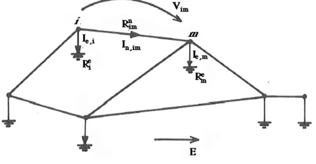
Since geoelectromagnetic variations are slow compared, for example, to the 50- and 60-Hz frequencies used in elec-tric power transmission, a dc modeling of GICs is accept-able (at least as a first approximation). Figure 1 gives a schematic view of a network having N discrete nodes, called stations, earthed by resistances Rie(i = 1, . . . ,N).
The resistance of a conductor line connecting stationsiand
m (i, m = 1, . . . ,N) is denoted by Ri mn . Lehtinen and
Pirjola (1985) derived the following formula for the N ×
1 column matrixIe, which consists of GICs, denoted byIe,m
(m=1, . . . ,N), and called the earthing GICs, to (from) the Earth (with the positive direction into the Earth) at the sta-tions:
Ie=(1+YnZe)−1Je (1)
This equation, which has been presented in many other pub-lications as well (e.g. Pirjola, 2005a, 2007, 2008a), provides a solution for the engineering part of a GIC calculation. The symbol1is an N × N unit identity matrix. The N × N
earthing impedance matrixZeand theN ×N network
ad-mittance matrixYn, as well as theN×1 column matrixJe, which includes the information about the geoelectric field, are defined below.
Multiplying Ie by Ze gives the voltages between the earthing points and a remote earth associated with the flow of the currentsIe,m(m=1, . . . ,N). Including the voltages
in anN×1 column matrixUcur, we thus have
Ucur=ZeIe. (2)
(Following the original notation by Lehtinen and Pirjola (1985), the subscript ‘cur’ indicates that voltages associ-ated with earthing currents are considered.) By the reci-procity theorem,Zeis symmetric. If the stations are distant
enough, thereby making the effect of one earthing current on the voltage at another station negligible,Zeis simply
di-agonal, with the elements equaling the earthing resistances
Re
Fig. 1. Network consisting ofNnodes, called stations, earthed by resistancesRie(i=1, . . . ,N). The resistance of a conductor line between stationsi
andm(i,m=1, . . . ,N) is denoted byRn
i m. An external geoelectric fieldEproduces geomagnetically induced currents (GICs) to (from) the Earth
denoted byIe,iand in the conductors denoted byIn,i m. The GICs are calculated by using the geovoltagesVi mobtained by integratingEalong the
conductors. This figure is a slightly modified version of figure 1 by Lehtinen and Pirjola (1985).
as the definition ofZe. The voltages included inUcur are physically associated with the electric field that produces a part of the (telluric) currents driven by the geoelectric field flowing through the earthed network.
The matrixYnis defined by
(i=m):Yn,i m = −
1
Ri mn
, (i =m):Yn,i m = N
k=1,k=i
1
Rni k
(3) which directly shows thatYn is a symmetric matrix. The elements Je,m(m=1, . . . ,N) of the column matrixJeare
Je,m= N
i=1,i=m Vi m Ri mn
(4)
The geovoltageVi m is produced by the horizontal
geoelec-tric fieldE, which is external from the viewpoint of the net-work in the engineering part of a GIC calculation. Thus,
Vi m is obtained by integrating E along the path defined
by the conductor line from station i to station m(i,m =
1, . . . ,N):
Vi m =
m
i
E·ds (5)
Generally, the geoelectric field is rotational, which implies that the integral in Eq. (5) is path-dependent, and the inte-gration route has to correspond to the conductor between
i andm(Boteler and Pirjola, 1998). Equation (1) directly shows that, assuming perfect earthings (“pe”), i.e.,Ze= 0, the GICs included inIeequal the elements ofJe, called the “pe” earthing currents.
Additional details associated with the derivation of Eqs. (1)–(5) are given by Lehtinen and Pirjola (1985). A formula for the GIC flowing in a conductor between sta-tions i andm (i, m = 1, . . . ,N), denoted by In,i m, can
also be derived (Lehtinen and Pirjola, 1985; Pirjola, 2007, 2008a), but this formula is less important in practice than Eq. (1) because the earthing GICs create problems by sat-urating power system transformers. Referring to the elec-trical circuit theory, we can say that the voltages Vi m and
those in Ucur correspond to the open-circuit electromotive force and the voltage drop in a battery, respectively, when the currentsIn,i min the conductors are considered.
When applying Eqs. (1)–(5) to calculating GICs in a real three-phase power system earthed via transformer neutrals at stations, the three phases are usually treated as one circuit element. The resistance of this element is then one third of that of a single phase, and it carries a GIC threefold higher than the current in a single conductor. For convenience, the (total) earthing resistances of the stations are defined to in-clude the actual earthing resistances, the transformer resis-tances, and the resistances of possible neutral point reactors (or any other resistors) in the earthing leads of transformer neutrals (all resistances in series). It should be noted that the technical reason for installing neutral point reactors is to decrease possible earth-fault currents, which is important for the safety of the power system. In terms of GICs, a neutral point reactor just provides an additional resistance in the earthing lead as a “spin-off”. M¨akinen (1993) and Pirjola (2005a) describe the application of Eqs. (1)–(5) to a power grid in further detail.
Here, I use the Cartesian coordinate system standard in geoelectromagnetics with thex yplane lying at the Earth’s surface and the x, y, and z axes pointing to the north, to the east, and downwards, respectively. The horizontal geoelectric field E = (Ex,Ey)is assumed to be known
at M grid points. In this study, we do not specify the details of the grid, except that its size and location have to enable the estimation of the electric field at all points of the network in which the GICs are investigated. The grid may be either regular or irregular, it can be rectangular or it may follow the latitudes and longitudes, and so on. For example, Wiket al.(2008) made a GIC calculation of the southern Swedish 400-kV power system using an 88-point grid (see their Fig. 2). The voltagesVi m are assumed to be
linear combinations of the values of the field components
Ex,kandEy,kat the grid points (k=1, . . . ,M):
Vi m = M
k=1
λi m
k Ex,k+ηi mk Ey,k
Fig. 2. Finnish 400-kV electric power transmission grid in its configu-ration valid in October 1978 to November 1979 (Pirjola and Lehtinen, 1985; Pirjola, 2005a). The names of the stations numbered from 1 to 17 are given in Table 1.
The coefficientsλi m k andη
i m
k have the dimension of length.
They depend on the numerical method of computing the in-tegral in Eq. (5), which involves both the interpolation from the grid pointsktox,yvalues lying at the conductor and the numerical integration itself. It is clear that the coefficients λi m
k andη i m
k decrease with increasing distance from the grid
pointkto the conductor connecting stationsiandm. Differ-ent techniques exist for the interpolation. The only implicit assumption included in Eq. (6) is that the linear dependence on the geoelectric field components is maintained (which is a very natural requirement). In this paper, however, I will not go into the details of the numerical computations ofλi m
k andη i m
k because the purpose of presenting Eq. (6) is
to derive a simple linear relationship between the geoelec-tric field and the GICs rather than to provide detailed in-structions and advice for numerical calculation techniques ofλi m
k andη i m
k . Moreover, the examples of the calculation
in Sections 4 and 5 refer to Eqs. (1)–(5) under a uniform geoelectric field.
Substituting Eq. (6) into Eq. (4) gives
Je,m=
From Eqs. (1) and (10), I then obtain
Ie=GE (11)
where the N ×2M matrix(1+YnZe)−1Ais denoted by G. The line and earthing resistances of the power grid are included in the matricesYnandZe. The matrixA charac-terizes the geometry of the network and the numerical com-putation of the voltages in Eq. (5), and it is also affected by the line resistances via Eq. (8). Separating the influences of the different factors by analyzing the matrixGis obviously a challenge in practice.
Although the timetis not explicitly included in the above discussion, the matrices E = E(t) and Ie = Ie(t) are functions of time. The matrixGdoes not depend on time (except for the fact that it varies with possible changes in the power system configuration or resistances, but it is a different issue). ConsideringLtime moments, we may still use Eq. (11), butIeis an N ×L matrix andEis a 2M × L matrix, with the columns corresponding to consecutive times. Let us then denote a single row of the matrixIebyg
and the corresponding row of the matrixGbyW. We thus refer to a particular station of the network, for example, one equipped with GIC measurements. The rowsgandWare 1 ×Land 1×2Mmatrices, respectively, and
g=WE (12)
3.
Effect of Changing the Value of an Earthing
Resistance on GICs at a Station
Letaandbdenote a GIC at a site in a power system pro-duced by a uniform northward or a uniform eastward geo-electric field of 1 V/km, respectively. Then, due to linearity, a GIC created by any uniform horizontal geoelectric field can be expressed as
GIC(t)=a Ex(t)+bEy(t) (13)
where the north and east components of the field, as well as GIC, are regarded as being dependent on the timet. A unit of a and b is expressed as amperes times kilometer per volt (A km/V), when ExandEyare expressed in volts
per kilometer (V/km) and the GIC is expressed in amperes. Considering separate time momentst =t1,. . .,tL, Eq. (13)
is actually a special case of Eq. (12) withM =1.
Equation (13) can also be applied to an experimental de-termination of the coefficientsa andb by using measured GIC data together with geoelectric field values computed from geomagnetic recordings (compare the end of Sec-tion 2; see, for example, Wiket al., 2008). The values of
aandbobtained by measurements are often different from the values by a model calculation performed with a uniform field of 1 V/km because the geoelectric field significantly depends on the Earth’s conductivity. However, the ratioa/b
is expected to be the same for both the experimental and the-oretically calculated coefficients. The ratio indicates the rel-ative importance of the two geoelectric components for the GIC at the considered site and depends on the grid configu-ration and resistances (see, for example, Wiket al., 2008). In practical situations, the calculated geoelectric field am-plitudes may be scaled to incorrect values due to lack of the precise ground conductivity data, but the two geoelectric components should obtain the correct relative weight when the calculated values are fitted to the measured GIC data.
Based on Eq. (1), I now investigate the effect of the (total) earthing resistance Rej of a given station j (j =1, . . . ,N)
on the ratioa/bassociated with the earthing GIC,Ie,jat the
same station. In practice, such a study may be useful when we cannot obtain reliable information on an additional resis-tor in the earthing lead of a transformer neutral during GIC measurements. The diagonal elementsZe,iiof the earthing
impedance matrix equal the resistancesRe
i (i =1, . . . ,N).
As mentioned in Section 2, the total earthing resistances of the stations include the actual earthing resistances, the transformer resistances, and the resistances of any resistors in the earthing leads of transformer neutrals. Based on the definition of Ze, it is clear that the off-diagonal elements ofZeare associated with the actual earthing resistances of the stations, which implies some coupling with the diago-nal elements as well. However, we now assume that possi-ble changes in the (total) earthing resistance Rejconsidered
do not refer to the actual earthing resistance, which agrees with thinking of an installation or a removal of a resistor in the neutral lead. Consequently, the only quantity affected by the change and included in the GIC calculation is the elementZe,j j(=Rej).
where the symbol δmp stands for the Kronecker delta (=
1 if m = p, and = 0 if m = p). Equation (14) shows that Ze,j j only affects the elements ofDthat lie in the jth
column, i.e. p = j. (In fact, all elements Ze,r j (r =
1, . . . ,N) only directly contribute to the jth column of
D but because Ze,r j = Ze,jr indirect effects also appear
elsewhere.) Consequently, the cofactors of the elements in the jth column ofDdo not depend on Ze,j j. From the
elementary matrix calculus, we know that the inverse ofD, needed in Eq. (1), is obtained by transposing the matrix composed of the cofactors of D and by dividing by the determinant of D(= det(D)). Thus, Ze,j j contributes to
By using the above-mentioned facts,
Ie,j = terisk means transposing.) It is important that the elements ψj i included in Eq. (16) are not affected by Ze,j j(= Rej).
According to Eqs. (4) and (5), the column matrixJeis in-dependent of all earthing resistances, includingRej.
Conse-quently, the effects of possible changes ofRejonIe,j, i.e., on
the earthing GIC at the site jconsidered, only come by the term det(D) in Eq. (16). The elements Je,i (i =1, . . . ,N)
introduce the information on the geoelectric field.
It thus follows that if Ie,j is calculated in two different
geoelectric field situations, expressed byJe,i(1)andJe,i(2)
(i = 1, . . . ,N), and the results are Ie,j(1)andIe,j(2), the
ratio Ie,j(1)/Ie,j(2)is not affected by changes in Rej. For
example, we obtaina =Ij(1)andb =Ij(2)for a uniform
northward and eastward geoelectric field of 1 V/km, as discussed above. Thus, the ratio a/b at each station is independent of the installation or removal of an additional resistor in the neutral point of the transformer.
4.
Test Model for GIC Calculations
For example, the Mesh Impedance Matrix Method (MIMM) and the Network Admittance Matrix Method (NAMM), both of which also refer to load-flow calculation techniques traditionally used by electric power industry, are applicable to GIC computations (Boteler and Pirjola, 2004). NAMM can be shown to be equivalent with the method developed independently by Lehtinen and Pirjola (1985), called LP and summarized in Section 2. In fact, LP is slightly more general as it allows the possibility of non-zero off-diagonal elements in the earthing impedance matrix. The computa-tions and formulas discussed in this paper are based on LP. For the comparisons, it is necessary to apply different GIC computation methods to the same power grid model. Figure 2, which refers to the Finnish 400-kV system in Oc-tober 1978 to November 1979 (Pirjola and Lehtinen, 1985; Pirjola, 2005a), is a recommendable choice for such a test model because the numbers of stations and transmission lines are high enough (17 stations and 19 transmission lines) but it is not too large to unnecessarily complicate the com-putations and analyses. (Note that between stations 11 and 13 there are actually two transmission lines but that in the GIC studies these are treated as a single line.) The earth-ing resistances of the stations and the resistances of the transmission lines are given in Tables 1 and 2, respectively. These data have also been presented by Pirjola and Lehti-nen (1985). As indicated in Section 2, the three phases are considered to be one circuit element, and the earthing resis-tances include the effects of both the station earthings and the transformers. No neutral point reactors (or other resis-tors) in the earthing leads are assumed. This is reasonable because most of the reactors were installed in the Finnish 400-kV system later than the period referred to in Fig. 2; as such, the test model remains simpler. Similar to Pirjola
and Lehtinen (1985), the earthing resistances of stations 16 and 17 are set equal to zero to approximately account for the connection to the Swedish 400-kV network. Thus, the currents Ie,16 and Ie,17 are actually not earthing GICs but
include currents that flow between the Finnish and Swedish systems.
Table 1 also gives the east and north coordinates of the stations in kilometers in a Cartesian coordinate system. (The origin located southwest of Finland does not play any role because only the relative positions of different parts and sites of the power grid are important.) The coordinates have been simply measured from a map and, therefore, possibly contain small inaccuracies. The resistance values presented in Tables 1 and 2 are based on information received from the power company in the beginning of the 1980s when GIC model calculations were initiated in Finland. In particular, the resistance data given in Table 1 may include approxi-mations. The power grid model provided by Fig. 2 and Ta-bles 1 and 2 is sufficient for GIC calculation tests, although the data of the model are slightly different from those of the old Finnish 400-kV system.
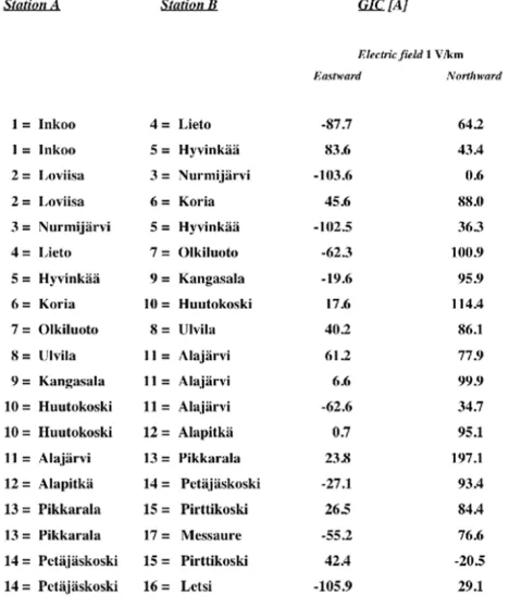
Based on the formulas given in Section 2 and the coor-dinate and resistance data expressed in Tables 1 and 2, Ta-ble 3 gives GICs that flow to (positive) or from (negative) the Earth at the stations of the grid considered under a uni-form eastward and a uniuni-form northward geoelectric field of 1 V/km. Table 4 presents GICs in the transmission lines (as positive from station A to station B). The GICs in these lines are calculated using the formula given, for example, by Pirjola (2008a) (see Section 2). In the present calcula-tion, I assumed that the earthing impedance matrix Ze is
Table 3. GICs at the stations of the Finnish 400-kV power grid shown in Fig. 2 under northward and eastward 1-V/km uniform horizontal geoelectric fields. GICs flowing to (from) the Earth are defined as positive (negative).
Table 4. GICs flowing between stations A and B (as positive from A to B) in the lines of the Finnish 400-kV power grid shown in Fig. 2 under northward and eastward 1-V/km uniform horizontal geoelectric fields.
Ze, too, but such a complication is neglected now.)
Tables 3 and 4 show that GICs in the lines tend, on av-erage, to exceed those through transformers. The means of the absolute values of the GICs in Table 3 are 41.9 A
(eastward) and 38.9 A (northward), and the corresponding values for Table 4 are 51.3 A (eastward) and 75.7 A (north-ward). This result is in agreement with the theoretical calcu-lation using an ideal system and the numerical computation using the Finnish 400-kV grid (Pirjola, 2005b). The GICs flowing through several earthings concentrate in lines in the middle of the network. As a result of this, the average GICs in the lines exceed the average earthing GICs. A compar-ison of Tables 3 and 4 with the GIC results given by Pir-jola and Lehtinen (1985) reveals small differences. This is due to the fact that the calculations discussed by Pirjola and Lehtinen (1985) were based on another earlier measurement of the station coordinates from a map, and there are minor deviations. Although the GIC magnitudes in Tables 3 and 4 vary largely from site to site, the same order of GICs was measured in the Finnish high-voltage system during geo-magnetic storms (Elovaaraet al., 1992). This provides an indirect verification of the validity of the calculations, al-though an exact agreement with a space storm event cannot be presumed because real geoelectric fields are not precisely uniform and equal to 1 V/km northwards or eastwards.
5.
Properties of the Transfer Matrix
Equations (1) and (4) express the GIC flowing through transformers to (from) the Earth in terms of the voltages associated with the horizontal geoelectric field along the transmission lines expressed by Eq. (5). The matrix formu-las (11) and (12) give a direct relation between GICs and the geoelectric field. Although these formulas look simple, their interpretation is complicated because the transfer ma-tricesGandWinclude the network parameters as well as the integration of the geoelectric field.
Let us now consider in greater detail the N × N ma-trix(1+YnZe)−1 appearing in Eq. (1) and denoted byC.
According to formulas (1) and (4), Cplays the role of a transfer matrix between the geovoltages and the earthing GICs. Perfect earthings (i.e.,Ze = 0), makeCthe iden-tity matrix so that the earthing GICsIeequal the “pe” cur-rentsJe(see Section 2). Lehtinen and Pirjola (1985) also give another interpretation of the equations derived for the currents produced by the geoelectric field in the earthings and the conductor lines by replacing the geoelectric field with an external injection of the “pe” currents Je,i into the
nodes (i = 1, . . . ,N). Although it is not said explic-itly, this formulation clearly corresponds to the use of Nor-ton’s equivalent current sources instead of geovoltages in the transmission lines (see also Boteler and Pirjola, 2004). The external injection results in a correct formula (1) for the earthing GICs, but the “pe” line GICs (= Vi m/Ri mn ; i, m = 1, . . . ,N) have to be added to the currents resulting from the injection. Consequently, if we do not think about an external injection but feed the “pe” currents Vi m/Ri mn
along the existing lines, no special addition is needed any more.
Based on Eq. (4) and on the relationsVi m = −Vmi and Rn
i m = Rmin , we easily obtain that the sum of the “pe”
currentsJe,i (i =1, . . . ,N) is zero. (It should be noted that
the sum of the earthing GICs Ie,m (m =1, . . . ,N) is zero
flows into and out of the network. However, the injections at the nodes are obviously independent of each other, which means that the current fed into (from) a single station flows in the form of earthing GICsIe,m(m=1, . . . ,N) to (from)
the Earth. Taking into account the equation
Ie=(1+YnZe)−1Je=CJe (17)
it can be seen that the part of an injected current Je,i that
is associated with the earthing GICIe,misCmi Je,i (i,m=
1, . . . ,N). Consequently,
Je,i = N
m=1
CmiJe,i ⇒ N
m=1
Cmi =1 (18)
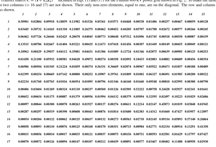
i.e., the sum of the elements in every column ofCis equal to one. This can be easily verified numerically by consid-ering, for example, the Finnish 400-kV grid introduced in Section 4, for which N =17. The matrixCfor this spe-cial case is presented in Table 5 (without showing the last two columns). It should be emphasized that although the earthing impedance matrixZeis assumed to be diagonal in the present numerical calculations for the Finnish 400-kV system, the result on the sum of the column elements inC
is always true because the theoretical derivation of Eq. (18) does not include any assumptions ofZe.
As in Section 3, the matrix1+YnZeis denoted byD,
i.e.,C=D−1. Thus, referring to Eq. (16), we can write
C= 1
det(D)[cof(D)]
∗ (19)
As, similarly to Section 3, the elements of [cof(D)]∗ are
denoted byψj k(j,k=1, . . . ,N), Eqs. (18) and (19) give
1 det(D)
N
m=1
ψmi =1 (20)
for all values of i = 1, . . . ,N. By the definition of a determinant,
det(D)= N
m=1
Dkmψmk (21)
for all values ofk = 1, . . . ,N. Equations (20) and (21) result in a special property of the matrixD = 1+YnZe, which fori =kcan be written as
N
m=1
(1−Di m)ψmi=0 (22)
for all values ofi = 1, . . . ,N. Finally, it is worth noting that although1,Yn, andZeare symmetric, the matricesC
andDneed not be symmetric (see Table 5). Thus, for ex-ample, the sums of the elements in the rows ofCgenerally differ from one.
The matrixCfor the Finnish 400-kV power system can now be considered. Table 5 shows that on each row of
Cthe largest element is on the diagonal. When the GIC process is described by the injection of the “pe” currents
Je, each earthing GICIe,m(m=1, . . . ,17) gets its greatest
Table 6. Elements C(10,j)(j = 1, . . . ,17) of the tenth row of the transfer matrixC=(1+YnZe)−1included in Eqs. (1) and (17) for the Finnish 400-kV power grid shown in Fig. 2. The elements are arranged in order of value. The distance is given a distance between station 10 and stationj. The neighborhood number is the number of stations from station 10 to station j: it is 1 for the nearest stations, 2 for the second nearest stations, and so on.
Je,i(i =1, . . . ,17) flows into (from) the Earth at this same
stationi. The exception can be explained by the facts that stations 3 and 5 lie very close to each other and the earthing resistance at station 3 is larger than at station 5, so a large part of the current injected at station 3 has an easy path to go into (from) the Earth at station 5. The only non-zero elements in columns 16 and 17 (not shown in Table 5) of the matrix C are the ones on the diagonal. This results from the zero earthing resistances at stations 16 and 17, which lead to the direct flow of the “pe” currents injected at these stations to (from) the Earth at the same sites. It is, however, worth noting that as the rows 16 and 17 also have non-zero off-diagonal elements, the currents Ie,16 andIe,17
receive contributions from other injections as well. (Note the comment of the nature ofIe,16andIe,17in Section 4.)
In general, the value of an element away from the diag-onal becomes small in the matrixC. This result, together with the numbering of the stations shown in Fig. 2, which implies that a small difference in the numbers generally means that the particular stations do not lie in very distant areas of the grid, indicates that remote parts of the network do not interact to any great extent. In other words, if earth-ing GIC values at a particular station are of interest, then it is sufficient to just take into account the neighborhood of the station. As an example, we consider the tenth row of the matrixC, which gives the value ofIe,10in terms of the
“pe” currents Je,i (i = 1, . . . ,17). (We could, of course,
consider any other row as well, but this particular row is chosen just because it refers to the station Huutokoski, at which Finnish GIC recordings were started in the 1970s (Pirjola, 1983).) Table 6 shows C(10,j)(j = 1, . . . ,17) arranged in order with its value. The corresponding value
of jand the distance between stations 10 and jas well as a “neighborhood number” are also given. The neighborhood number is the number of stations from station 10 to station
j: it is 1 for the nearest stations, 2 for the second nearest sta-tions, and so on. We clearly see that the elementsC(10,j)
generally decrease with both an increasing distance and an increasing neighborhood number. A closer look at Table 6 reveals that the neighborhood number plays a more impor-tant role for the elementsC(10,j)than the distance. Conse-quently, only the nearby part of the grid affects GICs at sta-tion 10. This result is in full agreement with the conclusion presented by Pirjola (2005a), who considered an idealized linear network and the Finnish 400-kV power grid.
The matrixC=(1+YnZe)−1has no explicit dependence on the distances between the stations or on the neighbor-hood numbers, but the influences come by the resistances
Re
i(i = 1, . . . ,17) and Ri mn (i,m = 1, . . . ,17). If the
neighborhood number between two stations becomes large, the “pe” current injected at one of them mostly goes into (from) the Earth before it reaches the other. This makes the corresponding element of the matrixCsmall. In any case, the currents always find the paths with the smallest resis-tance, which may lead to an explanation, for example, for the smaller value ofC(10,j)for j =8 than for j = 3 or 15 even though the neighborhood number of station 8 is less than that of stations 3 and 15. A large part of the injected currentJe,8goes, in addition to station 8 itself, to (from) the
Earth at station 7 with a small earthing resistance (Table 1). This explanation is supported by the large elementC(7,8) (Table 5). I have conducted this study using station 10, but the conclusions are clearly more generally valid. The earthing impedance matrixZeis assumed to be diagonal in
these calculations, but it is an irrelevant issue in this study because Pirjola (2008a, b) show that the off-diagonal ele-ments ofZeare of minor importance in practice. Thus, the
assumption ofZeto be diagonal obviously has no essential effect on the results in this paper.
6.
Concluding Remarks
“Geomagnetically induced currents” in electric power transmission grids and in other conductor networks are pro-duced by space storms that result from solar activity. Re-search on GICs has a lot of practical relevance because the GICs may cause problems to the systems and their opera-tion. The GICs play a particularly important role at high latitudes, but GIC magnitudes and possible harmful effects also depend on the technological structures and details of the networks, so the GICs should be taken into account at lower latitudes as well. Furthermore, the continuously in-creasing dependence of people on reliable technology em-phasizes the practical significance of the GICs and other space weather issues.
because it is affected both by the numerical computation of the geovoltages and by the resistances of the system. The separation of these two contributions is obviously not easy in practice.
This paper also provides new theoretical and numerical analyses of the properties of the transfer matrix between the geovoltages and the earthing GICs in a power system. A particular result, which is important in practice, is that the ratio of the GICs flowing to (from) the Earth at a station under two different geophysical situations is independent of the total earthing resistance at this station. The studies made in this paper aim at a better understanding of the phys-ical processes associated with the GICs. This is particularly achieved when describing the flow of GICs by assuming that the geoelectric field is replaced by the injection of “pe” currents into the network. An important result obtained by analyzing the behavior of the elements of the transfer ma-trix in this paper is that, when considering GICs at one site, model calculations can be limited to a smaller grid around the site. This is a confirmation of earlier conclusions drawn in a different way. Numerical computations discussed in this paper refer to an old configuration of the Finnish 400-kV electric power transmission grid. I believe that this par-ticular system is useful for testing different GIC calculation techniques, algorithms, and programs.
Acknowledgments. The author wishes to thank Dr. Ari Viljanen (Finnish Meteorological Institute) and Mr. Magnus Wik (Swedish Institute of Space Physics) for several inspiring and useful discus-sions associated with the items included in this paper and for the collaboration in the GIC research. The many valuable, careful, and constructive comments by the referees of the manuscript are grate-fully acknowledged. A revision of the manuscript according to the referees’ suggestions clearly improved and clarified the paper.
References
Bolduc, L., GIC observations and studies in the Hydro-Qu´ebec power system,J. Atmos. Sol.-Terr. Phys.,64(16), 1793–1802, 2002.
Boteler, D. H. and R. J. Pirjola, Modelling Geomagnetically Induced Cur-rents produced by Realistic and Uniform Electric Fields,IEEE Trans. Power Delivery,13(4), 1303–1308, 1998.
Boteler, D. H. and R. Pirjola, GIC Modelling,Technical Report for Real-Time GIC Simulator, ESA Space Weather Pilot Project, ESTEC Contract Number 16986/03/NL/LvH, European Space Agency (ESA), 27 pp., 2004.
nerability of Electric Power Grids, 2004.
Kappenman, J. G. and V. D. Albertson, Bracing for the geomagnetic storms,IEEE Spectrum, March 1990, 27–33, 1990.
Lanzerotti, L. J., D. J. Thomson, and C. G. Maclennan, Engineering issues in space weather, inModern Radio Science 1999, edited by M. A. Stuchly, 25–50, International Union of Radio Science (URSI), Oxford University Press, 1999.
Lehtinen, M. and R. Pirjola, Currents produced in earthed conductor net-works by geomagnetically-induced electric fields,Ann. Geophys.,3(4), 479–484, 1985.
M¨akinen, T., Geomagnetically induced currents in the Finnish power transmission system, Finnish Meteorological Institute, Geophysical Publications, No. 32, Helsinki, Finland, 101 pp., 1993.
Molinski, T. S., Why utilities respect geomagnetically induced currents,J. Atmos. Sol.-Terr. Phys.,64(16), 1765–1778, 2002.
Pirjola, R., Induction in power transmission lines during geomagnetic dis-turbances,Space Sci. Rev.,35(2), 185–193, 1983.
Pirjola, R., Effects of space weather on high-latitude ground systems,Adv. Space Res.,36(12), doi:10.1016/j.asr.2003.04.074, 2231–2240, 2005a. Pirjola, R., Averages of geomagnetically induced currents (GIC) in the
Finnish 400 kV electric power transmission system and the effect of neutral point reactors on GIC,J. Atmos. Sol.-Terr. Phys.,67(7), 701– 708, 2005b.
Pirjola, R., Calculation of geomagnetically induced currents (GIC) in a high-voltage electric power transmission system and estimation of ef-fects of overhead shield wires on GIC modelling,J. Atmos. Sol.-Terr. Phys.,69(12), 1305–1311, 2007.
Pirjola, R., Study of effects of changes of earthing resistances on geomag-netically induced currents in an electric power transmission system, Ra-dio Sci.,43, RS1004, doi:10.1029/2007RS003704, 13 pp., 2008a. Pirjola, R., Effects of interactions between stations on the calculation of
geomagnetically induced currents in an electric power transmission sys-tem,Earth Planets Space,60, 743–751, 2008b.
Pirjola, R. and M. Lehtinen, Currents produced in the Finnish 400 kV power transmission grid and in the Finnish natural gas pipeline by geomagnetically-induced electric fields,Ann. Geophys.,3(4), 485–491, 1985.
Pulkkinen, A., S. Lindahl, A. Viljanen, and R. Pirjola, Geomagnetic storm of 29–31 October 2003: Geomagnetically induced currents and their re-lation to problems in the Swedish high-voltage power transmission sys-tem,Space Weather,3, S08C03, doi: 10.1029/2004SW000123, 19 pp., 2005.
Watermann, J., The magnetic environment—GIC and other ground effects, inSpace Weather, Research Towards Applications in Europe, edited by J. Lilensten, Springer, Chapter 5.0, 269–275, 2007.
Wik, M., A. Viljanen, R. Pirjola, A. Pulkkinen, P. Wintoft, and H. Lundstedt, Calculation of geomagnetically induced currents in the 400 kV power grid in southern Sweden,Space Weather,6, S07005, doi:10.1029/2007SW000343, 11 pp., 2008.