Volume 2010, Article ID 641632,14pages doi:10.1155/2010/641632
Research Article
An Information-Theoretic Approach for Energy-Efficient
Collaborative Tracking in Wireless Sensor Networks
Loredana Arienzo
Institute for the Protection and Security of the Citizen, Joint Research Centre, European Commission, Ispra, 21027 Varese, Italy
Correspondence should be addressed to Loredana Arienzo,[email protected]
Received 3 November 2009; Accepted 24 February 2010
Academic Editor: Xinbing Wang
Copyright © 2010 Loredana Arienzo. This is an open access article distributed under the Creative Commons Attribution License, which permits unrestricted use, distribution, and reproduction in any medium, provided the original work is properly cited.
The problem of collaborative tracking of mobile nodes in wireless sensor networks is addressed. By using a novel metric derived from the energy model in LEACH (W.B. Heinzelman, A.P. Chandrakasan and H. Balakrishnan, Energy-Efficient Communication Protocol for Wireless Microsensor Networks, in: Proceedings of the 33rd Hawaii International Conference on System Sciences (HICSS ’00), 2000) and aiming at an efficient resource solution, the approach adopts a strategy of combining target tracking with node selection procedures in order to select informative sensors to minimize the energy consumption of the tracking task. We layout a cluster-based architecture to address the limitations in computational power, battery capacity and communication capacities of the sensor devices. The computation of the posterior Cramer-Rao bound (PCRB) based on received signal strength measurements has been considered. To track mobile nodes two particle filters are used: the bootstrap particle filter and the unscented particle filter, both in the centralized and in the distributed manner. Their performances are compared with the theoretical lower bound PCRB. To save energy, a node selection procedure based on greedy algorithms is proposed. The node selection problem is formulated as a cross-layer optimization problem and it is solved using greedy algorithms.
1. Introduction
Wireless sensor networks (WSNs), which normally consist of hundreds or thousands of sensor nodes each capable of sensing, processing, and transmitting environmental infor-mation, are deployed to monitor certain physical phenomena or to detect and track certain targets in an area of interests [1]. The issue of tracking moving targets in WSNs has received significant attention in recent years [2–4]. As any other algorithm designed for sensor networks, a tracking algorithm should be: (1) self-organizing, i.e. it should not depend on global infrastructure; (2) energy efficient, i.e. it should require little computation and, especially, communication; (3) robust, i.e. it should not depend on noise and movement of the target; (4) accurate, i.e. it should work with accuracy and precision in various environments, and should not depend on sensor-to-sensor connectivity in the network; (5) reliable, i.e. it should be tolerant to node failures.
Tracking a target in sensor networks is mainly challeng-ing regardless of the energy consumption due to resource-constrained features of such a network. The minimization of energy consumption for a sensor network with target activities is complicated since target estimation involves collaborative sensing and communication between different nodes. The problem of selecting the best nodes for tracking a target in a distributed wireless sensor network was investigated since [5].
The main idea is for a network to determine participants
in asensor collaborationby dynamically optimizing the utility
function of data for a given cost of communication and computation.
the sensor node which will result in the smallest expected posterior uncertainty of the target state is chosen as the next node to contribute to the movement decision. Specially, minimizing the expected posterior uncertainty is equivalent to maximizing the mutual information between the sensor node output and the target state [6]. In [7], an entropy-based sensor selection heuristic is proposed for target localization in which a sensor node is chosen at each step and the observation of that node is incorporeted into the target location distribution using sequential Bayesian filering. Instead, the main idea underlying our approach is that the heuristics select an informative sensor such that the fusion of the selected sensor observation with the prior target location distribution would yield to minimize the overall energy consumption in a cluster while maximizing the mutual information between the sensor node observation and the target state in order to improve the quality of the tracking data. We show that properly selected nodes to collect measurements in a cluster head, we can save energy to maximize the sensor network lifetime, and we will compare our node selection algorithm with that of Kaplan [8,9].
1.1. Main Contribution. The main contributions are as
follows.
(i) By using the energy model in [10], we propose a novel energy-based metric to evaluate the energy consumption of node selection algorithms in a cluster of sensor nodes.
(ii) We formulate the node selection problem as a cross-layer optimization problem and determine the optimal solution by greedy algorithm.
(iii) We compare the proposed node selection algorithms with the existing literature.
(iv) We implement distributed tracking algorithms using particle filter method and we compare them with the existing literature.
Preliminary results of this work were published in the author references [11]. The remainder of this paper is organized as follows: inSection 1.2we describe the existing work. Section 2 provides the preliminary information by describing the model of the overall system, by introducing the energy-based metrics. Section 3 provides a concise review of some basic concepts and statistical model of the nonlinear dynamical system.Section 4describes the tracking algorithms and formulates the distributed tracking problem introducing a node selection rule. InSection 5we describe the optimization problem and provide solutions. Section 6 discusses the performances of proposed algorithms, while in Section 7, we draw the main conclusions.
1.2. Related Work. Many criteria influence the design of
energy-efficient tracking approaches, and a wide range of schemes have been proposed. This Section is devoted to provide an overview of existing energy-efficient techniques for tracking a target in a wireless sensor network.
Generally, the hierarchical structuresinclude tree-based, cluster-based, and prediction-based structures. The
tree-based approaches [12–15] use a hierarchy tree to represent
the sensors and record information about presence of the objects being detected by the sensors. Kung and Vlah [12] propose STUN (Scalable Tracking Using Networked Sensors), a scalable tracking architecture that employs hierarchical structure to allow the system to handle a large number of tracked objects. Additionally to the tree, Lin and Tseng [13] consider an in-network moving object tracking in a sensor network, consisting of two operations: location update and query. The drawback is the building of the tree as the target moves. Zhang and Cao [14,15] propose DCTC (Dynamic Convoy Tree-Based Collaboration). They introduce a message-pruning tree structure called convoy tree, which is dynamically configured to add and prune some nodes as the target moves and the tracking problem is formalized as a multiple objective optimization problem. The solution to the problem is a convoy tree sequence with high tree coverage and low energy consumption. Building such a convoy tree sequence requires global network information, and reconfiguration and maintenance of a convoy tree incurs considerable computational and communication overhead. As a result, the tree-based approaches are usually centralized and applied in the deployment phase of sensor networks.
Wang et al. [16] and Chen et al. [17] propose
cluster-basedtracking schemes. They envision a hierarchical sensor
network that is composed of (a) a static backbone of sparsely placed position-aware sensors which will assume the role of a cluster head (CH) upon triggered by certain signal events and (b) moderately to densely populated low-end sensors whose function is to provide sensor information to CHs upon request. In these schemes, sensors are grouped into clusters either statically or dynamically (upon detection of the target in the vicinity), and a cluster head collects information from its cluster members and determines the target location using either the trilateration technique [16] or the Voronoi diagram-based approach [17]. Both localization approaches aim to determine the exact location of the target at the expense of considerable computational overhead because of the potentially high number of nodes in the cluster.
From thetopology perspective, the tracking approaches could use a global or local knowledge about the location of every node in the network. As opposed to the tree-based schemes [12–15] that use a global information, the cluster-based schemes [16,17] rely on local topology knowledge to limit the scope of target’s location updates.
As to thesignal processing, the tracking approaches can be classified as centralized or distributed. Usually the tree-based schemes are centralized approaches, while the cluster-based schemes are distributed schemes in which the cluster head is
theleader nodein the processing. The works in [13,18] are
centralized approaches, while those in [3,4,14,16,19] are distributed approaches.
CH
Sink
Active low-end sensor node with radio and unknown position Inactive low-end sensor node with radio and unknown position Active sensor node with radio and known position
Target position at the timet
Target trajectory
T(t)
Figure1: Sensor network topology.
management addresses the problem of choosing informative sensors needed to obtain information about the target state and therefore maximize the network lifetime. Based on
the collaboration, the existing approach of target tracking
can be classified in driven and information-based. Zhao et al. [19] propose IDSQ (Information Driven Sensor Querying), in which the selection of the best node is based on a Mahalanobis distance that leads to a heuristic method favoring the sensors whose Euclidean distance to the target is small. In [7–9] the node selection problem has been addressed using an information-based approach. The main idea behind this approach is to optimize a utility function, representing the location accuracy, using entropy-based metrics.
As will be discussed in detail in the next sections, the main idea underlined our proposed information-theoretic approach is to optimize an utility function representing the overall energy in a cluster, using energy-based metrics, jointly to the mutual information between the sensor node observation and the target state.
2. System Model
We make the following assumptions about the sensor network. First, the network is composed of a single gateway (sink) node and multiple sources. Next, the network is modeled as a combination of (1) a static backbone of sensor nodes aware of their position which assume the role of a cluster head and (2) randomly distributed low-end sensors which sense a moving target and report data to CHs upon request. Finally, we assume that the network is composed of dynamic clusters, depending on the predicted target trajectory (see Figure 1). Indeed, to facilitate collaborative data processing in target tracking sensor networks, usually the sensors are aggregated in clusters, led by a CH.
The details of the clustering algorithm are out of the aim of this paper. In the following we will limit ourselves to consider only the intra-cluster communication issues.
We only highlight that to waste less power the cluster-head should be selected with a shorter distance to the target. The active sensor of the cluster, which will assume the role of cluster head, will predict the trajectory of a target by means of a particle filter based on the history of the target location and some observations which come from some active sensors in the cluster. These sensors in the cluster are chosen to minimize the overall energy consumption.
2.1. Energy Model. The main concept underlying the
pro-posed energy efficient tracking algorithm is that the CH should select the active neighbors with the goal of reducing the total energy needed to transmit its data through its radio. In this subsection we introduce two metrics based on energy consumption for a tracking task.
2.1.1. Energy-Based Metric. To describe the energy
con-sumption of a tracking algorithm for power-constrained sensor network, we use the energy model for wireless sensor networks introduced by Heinzelman et al. [10]. The energy consumption per bit at the physical layer is
E=ETx-elec+βdα+ERx-elec, (1) where ETx-elec is a distance independent term that takes into account overheads of transmitter electronics (PLLs, VCOs, bias currents, etc.) and digital processing;ERx-elecis a distance independent term that takes into account overheads of receiver electronics; finallyβdαaccounts for the radiated power necessary to transmit one bit over a distancedbetween source and destination, whereαis the exponent of the path loss (2≤α≤5).
According to [21] we assume that ETx-elec = ERx-elec =
Eelec. Hence, givenlbits of data, the overall energy consump-tion to transmit the packet oflbit between two nodes at a distancedwith a given received SNR can be expressed as
E(d,l)=2Eelec+Eamp·dα
·l, (2) whereEelec[Joule/bit] is the energy needed by the transceiver circuitry to transmit or receive one bit andEamp[Joule/(bit· mα)] is a constant which represents the energy needed to transmit one bit over a distancedto achieve an acceptable SNR at the destination.
This model assumes that the energy consumption is dominated by the radio communication rather than the computation. We refer to (2) as the energy-based metric.
2.1.2. Residual Energy-Based Metric. According to [22,23]
we propose another metric combining energy and remaining energy at nodes. Hence, if we refer to a link (i,j) with distance
d, the overall energy consumption to transmit al-bit packet between the nodeiand node jat a distancedwith a given received SNR can be expressed as
Ei j(d,l)=Er−
2Eelec+Eamp·dα
2.2. Network Model. In our analysis, we consider a network composed of randomly deployed sensor nodes which sense a moving target and forward the information into a position-aware sensor which acts as a data gathering node. The network is divided intoNc clusters each having Na nodes. Each sensor is equipped by a low data rate radio interface. The position-aware sensors are equipped by two radio trans-mitters, that is, a low data rate transmitter to communicate with the sensors, and a high rate wireless interface for CH-CH communication.
In our analysis, we assume to know the position of the CH (static node) and to estimate the distance of each neighbor with respect the CH. Many types of sensors provide measurements that are function of the relative distance between the sensor and the sensed object (e.g., acoustic sensors, sonar, etc.). We consider a common example, newly in [4], where sensors measure the power of a radio signal emitted by the object.
Therefore, we assume the log-normal shadowing model for the channel and we suppose that the power of a received signal decreases exponentially with the propagation distance:
Pr(d)=Pr(do)·
where Pr(d) is the received power at a receiver at distance
d from a transmitter, Pr(do) is the transmitted power at a reference distancedo,αis the path loss exponent (2≤α≤5), andXσ is the shadow fading component, withXσ Gaussian distributionN(0,σ).
Hence, the distance from the ith sensor of the cluster to the CH can be estimated as d = (Pr/Pa)−1/α, where Pr is the received signal strength in the sensor, and Pa is the (unknown) strength of the signal from the sensor.
3. Basic Concepts and Theoretical Bound
We begin our analysis with a concise review of some basic concepts and the models of a nonlinear dynamical system.
We consider the state estimation of a nonlinear dynami-cal system:
xk+1=fk(xk,wk),
zk=hk(xk,vk),
(5)
where, k is the discrete time index; xkRn is the state vector;zkRmis the observation vector;w
kis the zero-mean white Gaussian process noise with nonsingular covariance matrixQk;vkis the zero-mean white Gaussian measurement noise independent ofwkwith nonsingular covariance matrix
Rk;fkandhkare the (in general) nonlinear functions. The functions fk and hk may depend on time k. Further we assume that the initial statex0 has a known probability density functionp(x0). Let∇andΔbe operators of the first-and second-order partial derivatives, respectively,
∇xk=
Using this notation, the Fisher Information Matrix (FIM) given by [24] for this problem can be written as
J(xk)= −E
Δxk
xklogp(zk,xk) , (7)
where p(zk,xk) represents the joint probability density of (zk,xk) In the following sectionsJ(xk) is denoted byJk for brevity. The following proposition [25] gives an efficient method for computingJkrecursively.
Proposition 1. The sequence{Jk}of Fisher information
sub-matrices for estimating state vectors{xk}obeys the recursion:
Jk+1=D22k −D21k
3.1. Time-Invariant Model. We assume that the functions
fk(·,·) and hk(·,·) are time invariant (independent of k). Using this assumption and according to [25], the matrices
D11k ,. . .,D22k do not depend onk, and additionally fork → ∞, the matrixJkconverges to a matrixJ∞, which is given as a
solution to the following equation:
J∞=D22k −D21k
Note that (10) is a discrete-time algebraic Riccati equation. A common form of the Riccati equation is obtained if the recursion (8) is equivalently written as
Jk+1=D21k
which can be easily proved by simple algebraic manipula-tions. Then, putJk+1=Jk=J∞.
3.2. Model for State Estimation of a Nonlinear Dynamical
System. The problem of estimating the state vector of a
nonlinear dynamical system (i.e., single target tracking) can be formulated as follows. The state and the observations of the target of interest are assumed to follow the following model:
xk+1=Fkxk+Akwk,
zk=Hk(xk) +Bkvk,
wherexk,zk,wk, andvkwere introduced inSection 3. The matricesFk,Ak, andBk are independent of the state vector whereasHk is a function dependent of the state vector xk. From the assumption that the noiseswkandvkare Gaussian with zero mean and invertible covariances matricesQk and
Rk, respectively, and that the elements of the noise vectorswk andvk are independent and identically distributed (IID) it follows that the conditional densities can be written as
p(xk+1|xk)= 1
2π|Qi|·e
−(1/2)[xk+1−Fkxk]TQ−k1[xk+1−Fkxk],
p(zk|xk)= 1 2π|Qi|·e
−(1/2)[zk−Hk(xk)]TR−k1[zi−Hk(xk)]
(13)
In the derivation above, we assume that the system model is time-invariant, implying thatQ1=Q2= · · · =Qk=Qand
R1=R2= · · · =Rk=R. Consequently, from (13), we have
−logp(xk+1|xk)=c1+ 1
2[xk+1−Fkxk] TQ−1
k [xk+1−Fkxk],
−logp(zk|xk)=c2+ 1
2[zk−Hk(xk)] TR−1
k [zk−Hk(xk)], (14)
wherec1andc2are constants, and
D11k =E∇xk[xk+1−Fkxk]
TQ−1
k · ∇Txk[xk+1−Fkxk]
,
D12 k = −E
∇xk[xk+1−Fkxk]
T,
D22k =Q−k1+E−∇xk+1[zk+1−Hk+1(xk+1)]
T
·R−1
k+1∇Txk+1[zk+1−Hk+1(xk+1)]
.
(15)
4. Tracking Algorithms
The aim of this section is to describe the proposed cross-layer predictive tracking algorithm and to discuss that it can consistently reduce the energy consumption on sensors with respect to existent one-level location algorithms. As stated above, in this paper we use sequential Monte Carlo (SMC) approaches, also known as particle filtering [26, 27], for tracking a moving target while Kaplan [8,9] estimates the target location using a Kalman filter based on the current measurement at a sensor and the past history at other sen-sors. The particle filter provides simulation-based solutions to estimate the posterior distribution of nonlinear discrete time dynamic models. The main idea of particle filtering is to represent the required posterior distribution density by a set of random samples with associated weights and to compute estimates based on these samples and weights, updating them recursively in time using the sequential importance sampling (SIS) algorithm. As the number of samples becomes very large, the SIS filter approaches the optimal Bayesian estimate. A common problem with the SIS particle filter is the degeneracy phenomenon, since after a few iterations all the particles, with exception of one of them, will have negligible weight. Because of this phenomenon, resampling techniques
are used to eliminate particles that have small weights and to concentrate on particles with large weights. The particle filter using sequential importance resampling (SIR) techniques is known asbootstrap filteror SIR particle filter (PF). Therefore, in the following we use the SIR filter to achieve the tracking task. Moreover, we compare the performance of bootstrap filter with the unscented particle filter. Indeed, unfortunately even when resampling schemes are used, degeneracy may still be a problem. Using the prior distribution as importance distribution could lead to the degeneracy problem of the particles because the most recent observations are ignored. Samples may eventually collapse to a single point if, during the resampling stage, samples with high importance weights are duplicated an extremely large number of times. There have been numerous proposals to rectify the degeneracy problem improving the performance of the SIR particle filter [28]. Notable techniques include local linearization using the extended Kalman filter (EKF) [29, 30] or the unscented Kalman filter (UKF) to estimate the importance distribution [31]. A particle filter which uses UKF to generate the importance distribution is referred asunscented particle
filter(UPF) or sigma-point particle filter [31].
In this paper, we analyze the energy efficiency of particle filtering looking at collaborative and distributed schema for tracking a moving target.
4.1. Node Selection. We formulate the problem of distributed
tracking as a sequential Monte Carlo estimation problem. Assume that the state of a target we wish to estimate is
xk. Each new sensor measurementzk is combined with the current estimate p(xk | z1,. . .,zk−1), hereafter called belief state, to form a new belief state of the targetp(xk|z1,. . .,zk). The problem of selecting a sensor in order to provide greatest improvement to the estimation at the lowest cost becomes an optimization problem. We let Zk be all measurements that have already been used at time k in the inference of the current belief state and refer the sensor which holds the belief state as the leader node. The objective function for this optimization problem can be defined as a mixture of both information gain and cost. In the remainder of the section we consider the information gain, while the computation of the energy consumption cost is discussed in the next section. The information gain to select the sensorscan be defined asΦs(p(xk |Zk))=ΦUtility(p(xk+1 |Zk,zk+1,s)), wherezk+1,s is the new measurement from sensor s at timek+ 1. The utility function can be defined as the uncertainty of the target state reduced by the additional measurementszk+1,s[6], that is,Φs(p(xk |Zk))=Htarget(Zk)−Htarget(Zk,zk+1,s). Further-more, the utility function can be defined with the mutual informationΦUtility(p(xk+1,zk+1,s|Zk))=I(xk+1,zk+1,s|Zk), which means the information ofxk+1 conveyed by the new measurementszk+1,s[18].
available, the new belief or posterior is evaluated using sequential Bayesian filtering p(xk+1 |zk+1,s,Zk)∝ p(zk+1,s|
xk+1)p(xk+1|Zk).Without having the datazk+1,s, we need to compute the expected posterior distributionEzk+1,s(p(xk+1 | zk+1,s,Zk)). We can estimate the measurement zk+1,s from the predicted belief and compute the expected likelihood functionp(zk+1,s|xk+1)=
p(zk+1,s(νk+1)|xk+1)×p(νk+1|
Zk)dνk+1.Then, the expected posterior belief can be defined as follows:
pxk+1|zk+1,s,Zk
=pzk+1,s|xk+1
p(xk+1|Zk). (16)
The entropy of expected posterior distribution can be com-pute based on the discrete belief state{xkj,wkj}N
j=1[32], where
wkj is the importance sampling weight in the resampling step of the particle filters and N represents the number of weights namely the number of particles. According to (16), the expected posterior belief for sensorscan be represented by the discrete belief state {xkj,wkj+1,s}Nj=1 with the weights
wkj+1,sgiven by
wkj+1,s=p
zk+1,s|xkj+1
wkj+1. (17)
The entropy of the discrete belief state{xkj+1,wkj+1,s}Nj=1can be computed by
H= −
N
j=1
wkj+1,slogw j
k+1,s. (18)
This expected posterior entropy can be used as a criteria to select the best among the sensor candidates to maximize the information gain. The objective function expected to improve the estimation of the target is given by
Ns=arg max s∈Na
Φs
p(xk|Zk)
=arg max s∈Na
Htarget(Zk)−Htarget
Zk,zk+1,s
,
(19)
where Na indicates the set, with cardinality Na, of active nodes in the cluster that receive from the CH a signal exceeding a predetermined RSS threshold.
5. Energy Efficient Tracking
Let us consider the following location discovery protocol for a given snapshot. With reference to Figure 2, the targetT
periodically sends discovery signal, with period TM, to all the sensors of the network. We indicate withNs the set of active neighbor nodes that maximize the utility function as in (19). The subsetNd of desired anchor nodes needed for the localization algorithm will be chosen so as to minimize the energy consumption of the location discovery protocol. Then, each nodei ∈ Nstransmits the sensing information (the distance of the nodeifrom the target) to the CH which processes the data and updates the current target location.
CH i
di
dj
ri rj
j
T
Figure2: Location discovery protocol.
According to metric (2), the energy cost in the commu-nication with one sensori∈Nsis given by
Ei(ri,di)=
Eelec(Nd+ 2) +Eamp·diα · l TM
+Eelec(Nd+ 1) +Eamp·riα ·b,
(20)
wherebrepresents the bit rate (bit/s) between the CH and the neighbori,TM(s) is the period between two consecutive discovery signal of the target,rianddiare, respectively, the distance of the nodeifrom the CH and the target, andNd is the number of desired neighbors of the CH. Finally, in (20)EelecNd represents the energy needed at the neighbors to receive one bit. In the energy cost we have omitted the energy consumption in the path between the target and the CH due to the calibration phase of the clustering and we have considered only the communication between each node of the cluster and its cluster head.
On the other hand, according to the metric (3) and the location discovery protocol herein discussed, the energy cost in the communication with the sensoriNs, based on (20), is given by
Ui(ri,di)=2Er(i)−Ei(ri,di). (21) The total utility function, for all nodes in the setNs, is given by
UTOT(N s)=
i∈Ns
Ui(ri,di). (22)
As stated above, our objective is to select the optimal subsetNd ⊂ Nswhich maximizes the total utility function in (22), subject to a constraint of the cardinalityNd of said subset. This gives formally the following objective function and associated constraint:
Nd =arg max N⊆NsU
TOT(N) subject toN
Synopsis:[Nd,C,Etot,node,Eb,k]=Greedy(Ns,Nd). Given:Set of nodes in the clusterNs, number of desired
nodesNd.
Output:Set of desired nodesNd, new set of candidate nodes in the clusterC, total energy of the desired set Etot, last node selected in the current snapshotnode,
energy of this nodeEb, timek.
Initialize the candidate set: C=Ns
Ncand=0
Initialize the objective function: Etot=0
Randomly select a candidate nodei∈C
Emin=E(i)
NodeMin=i
while|Ncand|< Nddo foreachj∈C\ {i}do
if E(j)< Eminthen
Emin=E(j)
NodeMin=j
end if end for
node=NodeMin Eb=Emin
Etot=Etot+Emin
Ncand=Ncand∪ {NodeMin} C=C\ {NodeMin} end while
Nd=Ncand
Algorithm1: Greedy random node selection.
5.1. The Solution in the Static Scenario. To find the optimal
solution for such problem it is theoretically possible to enumerate the solutions and evaluate each with respect to the stated objective. However, from a practical perspective, it is infeasible to follow such a strategy because the num-ber of combinations grows exponentially with the size of problem.
Indeed, if we formulate our combinatorial optimization problem as an integer linear programming problem, the computational complexity consists of enumerating all the
Nd-node subsets, O(NaNd), and adding the computational complexity of the assignment problem,O(N3
d). In such cases, heuristic methods are usually employed to find good, but not necessarily guaranteed optimal solutions. More than one technique is applicable, that is, integer linear programming, graph theory, genetic algorithms, and greedy heuristics; see [33] for further details. Here we adopt the meta-heuristic greedy randomized adaptive search procedures (GRASP) [34], in which each iteration consists of two phases, a construction phase, in which a feasible solution is produced, and a local search phase, in which a local optimum in the neighborhood of the constructed solution is sought. The best overall solution is kept as the result.
The implementation of the optimal Greedy node selec-tion procedure is described inAlgorithm 1. It provides the set
Synopsis:[Nd,C,Etot]=BranchBound(Nd,C,Eb,node). Given:Number of desired nodesNd, candidate nodes
set of the clusterNa, energy boundEb, node related to the energy boundnode.
Output:Set of desired nodesNd, new set of candidate nodes in the clusterC, total energy of the desired set Etot.
Initialize the candidate set: Ncand= {node}
Initialize the objective function: Etot=Eb
while|Ncand|< Nddo foreachj∈C\ {i}do
if E(j)< Ebthen break else
Emin=E(j)
NodeMin=j
end if end for
Ncand=Ncand∪ {NodeMin} C=C\ {NodeMin}
Etot=Etot+Emin end while
Nd=Ncand
Algorithm2: Branch and bound algorithm.
of desired nodesNd, new set of candidate nodes in the cluster
C, total energy of the desired setEtot, last node selected in the current snapshotnode, energy of this nodeEb, and time
k.
5.2. The Solution in the Dynamic Scenario. In previous
sec-tions, we have considered the static version of the problem, namely, a snapshot model. In this section we extend the Greedy node selection procedure over multiple snapshots, so that we can select active nodes for the next measurement intervals. In a dynamic scenario, due to the target mobility, the distance di in (20) varies with the time and hence the total utility function (22) is a function of timek.
In the dynamic version of the optimization problem we use the Dynamic Programming [35], that is based on the idea of breaking down the problem into stages at which the decisions take place and finding a recurrence relation that takes us backward from one stage to the previous stage. For this purpose, a branch-and-bound method is developed, in which the branch refers to the partitioning process into stages, that are repeatedly decomposed until a solution is found or infeasibility is proved, and the bound refers to lower bounds that are used to construct a proof of optimality without exhaustive search. We introduce anenergy boundas in the following definition.
Definition 1. The energy bound is the maximum energy
Synopsis:[Nd,C,Etot]=DynamicSelection(Na,Nd). Output:Set of desired nodesNd, new set of candidate
nodes in the clusterC,total energy of the desired setEtot.
(1) The initial leader node does the following step: (a) draw initial samples{x0j,w0j=1}Nj=1of the target
from the prior information; (b) update the belief state
{x1j,w1}j Nj=1by the sensor fusion algorithm
based on the new measurementz1at the leader node
in the setNa; (c) compute the expected posterior belief state{x2j,w2,ji}Nj=1for each neighboor nodei
with the weightsw2,jicomputed by (17); (d) compute the entropy of the expected posterior belief state
{x2j,w2,ji}Nj=1for each neighboor nodeiby(18)
and determine the next best sensor, say (b) in the set Ns.
(2) [Nd,C,Etot,node,Eb,k]=Greedy(Ns,Nd) (3) Loop until time runs out:
(4) Prediction step and Update step of particle filtering to estimate the target’s trajectory. (5) Update the candidate setCduring the dynamic of
the target.
(6) [Nd,C,Etot]=BranchBound(Nd,C,Eb,node)
Algorithm3: Tracking algorithm.
Table 1: Computational complexity of the node selection algo-rithms.
Number of desired nodes Greedy Kaplan
1 O(Na−1) O((Na−1)2)
2 O(Na−2) O((Na−2)2)
· · · · · · · · ·
Nd O(Na−Nd) O((Na−Nd)2)
Algorithm 2shows pseudocode of an efficient implemen-tation of our branch-and-bound approach. It provides the set of desired nodes Nd, the new set of candidate nodes in the clusterC, and the total energy of the desired setEtot. Note that the total utility function of the desired set can be obtained from the following equation:
UTOT(N
d)=2ErNd−ETOT(Nd), (24) assuming that the nodes of the cluster have an even remaining energy, that is,
Er(i)=Er ∀iNd. (25)
Finally, inAlgorithm 3has been reported the overall tracking algorithm which combines the node’s selection procedures with the particle filtering algorithm.
6. Performance Evaluation
In this section, we investigate the performance of the overall target tracking system looking first at the node selection
Table2: Time to process greedy and Kaplan algorithms.
Number of desired nodes Greedy Time Kaplan Time
2 6.6639e−5 13.9816e−4
3 7.8829e−5 32.5238e−4
4 1.0095e−4 10.0543e−3
5 1.2099e−4 23.1352e−3
6 1.4041e−4 52.2764e−3
algorithm and then at the tracking algorithm and energy consumption.
6.1. Optimal Node Selection. In the following we compare
our greedynode selection algorithm with theKaplan
algo-rithm in [8,9]. The only difference between [8] and [9] is that in [8] the global topology knowledge is assumed, in which every active node reaches the entire network, while in [9] the only knowledge of the relative position to the target and the active nodes from the previous snapshot is required.Table 1shows the computational complexity of the proposed node selection algorithm and theKaplanalgorithm for each iteration. Hence, the computational complexity for all iterations is given by the following.
(i) Greedy computational complexity: Nd
i=0(Na −i) =
NaNd+Na−(Nd2/2)−(Nd/2).
(ii) Kaplan computational complexity: Nd
i=0(Na−i)2 =
N2
a(Nd+1)+(Nd(Nd+1)(2Nd+1))/(6)−2Na(Nd(Nd+ 1))/2.
Indeed, in the above analysis we have omitted the computational complexity of the initialization step of the Simplex algorithm, in which two nodes are chosen by exhaustive search. Definitely, due to computational com-plexity and because the simplex does not always find the global minimum, our approach outperforms the Kaplan algorithm.
As stated in Section 4.1, the node selection procedure is combined with the maximization of the utility function. Hence in our analysis the computational complexity of the problem in (19) needs to be considered, namely, O(NdNlogN) where N is the number of weights. Finally, the computational complexity for all iterations is given by Nd
i=1iNlogN.
In Table 2 the results of a runtime measurement are illustrated, conducted on a system with AMD Opteron XP Processor 250, approximately 2400 MHz frequency, and 4,00 GB RAM. Table 2 provides the execution time of the node’s selection algorithm versus the number of desired nodes usingNaequal to 10 andNequal to 100.
6.2. Estimation Bound for Range-Based Tracking. In this
Table3: Parameters of the model used for simulations.
Parameters Scenario 1 Scenario 2
Size 20 m2 200 m2
velocity 0.1 m/s 0.3 m/s
K 9 dB 9 dB
α 3 3
Eelec 10 nJ/bit 10 nJ/bit
Eamp 100 pJ/bit/m3 100 pJ/bit/m3
TM 2 sec 2 sec
b 10 bit/sec 10 bit/sec
l 8 bits 8 bits
ΔT 1 sec 1 sec
Process variance 1.0 1.8
Observation variance 0.3 0.3
particle number 100, 500 100, 500
given by ΔTthe length of the measurement interval.
Additionally, as observation model of the measurements, we use the log-normal shadowing model [37]. Hence, let
{αs,βs}be the fixed position of sensorsand letd
k = xk−
s1/2=[(α
k−αs)2+ (βk−βs)2](1/2)be the distance between the sensorsand the target; in a logarithmic scale the target-originated measurements are modeled by
Hk(xk)=K−10αlog(dk),
zk=Hk(xk) +Bkvk,
(27)
where the measurement noisevkaccounts for the shadowing effects and other uncertainties. The noisevk is assumed to be a zero-mean Gaussian with covariances valuesσ2
x =σy2=
σ2
o, and the sensor noises are assumed uncorrelated;Kis the transmission power, andα∈[2, 5] is the path loss exponent. Consequently, a straightforward calculation of (15) gives
D11
From (11), the recursion of information matrix can be written as
Substituting (30) in (29) the recursion of information matrix is given by
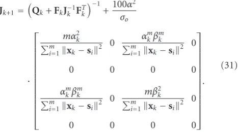
The initial information matrix required for the recursion is calculated from the prior probability density functionp(x0). We assume that the initial target state is a Gaussian random variable andx0 ∼N(x0,P0). Then, if the state is Gaussian with covarianceP0,Jkcan be recursively computed from the initial conditionJ0=P−01.
6.3. Tracking Accuracy. We implemented the node’s selection
algorithms and the particle filters in a Matlab simulator. We present simulation results for the scenarios illustrated in Table 3. Figure 3 shows the target trajectories for two different velocities, equal to 0.1 and 0.3 m/s, used in the experiment.
In Figures 4 and5, we have shown the PCRBs for the position, meaning that the (1,1) and (3,3) elements ofJ−1 are considered. Furthermore, we compare the PCRB with the root mean square errors of PF and UPF for different numbers
mof active nodes. It should be noted that the empirical error curves for the PF and the UPF closely match the theoretical PCRB for the problem considered. This means that the PF and the UPF appear to be efficient sequential estimators of the target state vector. The simulation results provide that the PCRB decreases as the number of active nodes increases. Note that in Figure 4(d), contrarily to the PCRB, the root mean square error of the two filters shows a divergence from the expected decreasing behavior. We believe it is due to the degeneracy phenomenon of particle filters; however, an additional investigation is needed.
0 2 4 6 8 10 12 14 16 18
20
T=1
T=200
x(meters)
y
(met
ers)
Actual trajectory Sensor nodes 0
2 4 6 8 10 12 14 16
(a) Scenario 1: target velocity=0.1 m/s
−250 −200 −150 −100 −50 0
T=1
T=200
x(meters)
y
(met
ers)
Actual trajectory Sensor nodes
−30 −20 −10 0 10 20 30 40 50
(b) Scenario 2: target velocity=0.3 m/s Figure3: Actual track of the target with different velocity.
0 20 40 60 80 100 120 140 160 180 200 0.05
0.15 0.25
0.1 0.2
Time (seconds)
RMSE
of
pr
ed
ic
ti
on
(m)
(a) 3 nodes
0 20 40 60 80 100 120 140 160 180 200
Time (seconds)
RMSE
of
pr
ed
ic
ti
on
(m)
0.06 0.08 0.12 0.14 0.16 0.18
0.1 0.2
(b) 4 nodes
RMSE PF RMSE UPF PCRB
0 20 40 60 80 100 120 140 160 180 200
Time (seconds)
RMSE
of
pr
ed
ic
ti
on
(m)
0.06 0.08 0.12 0.14 0.16 0.18 0.22
0.1 0.2
(c) 5 nodes
RMSE PF RMSE UPF PCRB
0 20 40 60 80 100 120 140 160 180 200
Time (seconds)
RMSE
of
pr
ed
ic
ti
on
(m)
0.06 0.08 0.12 0.14 0.16 0.18 0.22
0.1 0.2
(d) 6 nodes
0 20 40 60 80 100 120 140 160 180 200 0
0.5 1 1.5 2 2.5 3 3.5 4
RMSE
of
pr
edic
ti
on
(m)
Time (seconds)
(a) 3 nodes
0 20 40 60 80 100 120 140 160 180 200
RMSE
of
pr
edic
tion
(m)
Time (seconds) 0
0.5 1 1.5 2 2.5
(b) 4 nodes
0 20 40 60 80 100 120 140 160 180 200
RMSE
of
pr
edic
tion
(m)
Time (seconds) 0.2
0.3 0.4 0.5 0.6 0.7 0.8 0.9 1 1.1 1.2
RMSE PF RMSE UPF PCRB
(c) 5 nodes
0 20 40 60 80 100 120 140 160 180 200
RMSE
of
pr
edic
tion
(m)
Time (seconds)
RMSE PF RMSE UPF PCRB 0.2
0.3 0.4 0.5 0.6 0.7 0.8 0.9 1
(d) 6 nodes Figure5: Compared tracking error versus time with target velocity=0.3 m/s.
2 3 4 5 6
0.12 0.14 0.16 0.18 0.2 0.22 0.24 0.26 0.28
Number of selected nodes
RMSE
(met
ers)
PF DPF DSPIF
UPF DUPF
(a)
3 4 5 6
0.4 0.5 0.6 0.7 0.8 0.9 1
Number of selected nodes
RMSE
(met
ers)
PF DPF DSPIF
UPF DUPF
(b)
2 3 4 5 6 0.2
0.3 0.4 0.5 0.6 0.7 0.8 0.9 1
Number of selected nodes
Energ
y
consumpt
ion
(J
)
Greedy Kaplan
(a) Energy consumption of Kalpan and Greedy algorithms versus number of nodes
0.2 0.3 0.4 0.5 0.6
0.1 0.2 0.3
Energy consumption (J)
RMSE
(met
ers)
PF UPF
DPF DUPF
(b) RMSE versus Energy consumption for different tracking algorithms using Greedy selection
Figure7: Energy consumption comparison.
and the unscented particle filter have been implemented in both centralized and distributed manner using the node selection rules. The performance of the distributed PF (DPF) and distributed UPF (DUPF) is compared with the performance of the distributed sigma-point information filter (DSPIF) from [4]. Confidence intervals are not shown for the sake of clarity.
In Scenario1, nodes are randomly deployed on an area of 20 m×20 m and the target speed is 0.1 m/s (seeFigure 3(a)). In Figure 6(a) a process varianceσp equal to 1.0 has been used for the trajectory 3(a). Clearly, the centralized filter PF outperforms the distributed filter DPF in tracking quality because in the distributed algorithms nodes only have local knowledge. Also the RMSE of DUPF is always larger than that for UPF. On the other hand, as we will show, the energy consumption is higher for the centralized approach. Finally, DPF and DUPF outperform DSPIF.
In Scenario2, nodes are randomly deployed on an area of 200 m × 200 m and the target speed is 0.3 m/s (see Figure 3(b)).Figure 6(b) illustrates the root-mean-squared error (RMSE) on the position of the target, depending on the number of active nodes in the network.Figure 6(b) shows the RMSE for a process varianceσp equal to 1.8. Again the unscented particle filter with 100 particles gives best results than the bootstrap particle filter using 100 particles as it is clear in Figure 6(b). Simulation results indicate a decrease in tracking performance with increase of noise and fast target movement. Note that, in Figure 6(b), the values of the error when the number of desired nodes is equal two are omitted because in this case the filter diverges. Other simulation results that we have not reported, with target velocity equal to 0.5 and 1.0 m/s, show that to estimate the track when the velocity increases a high number of anchor nodes are needed. For each value of Nd, 10000 different random configurations were generated, where, for each configuration, we assume a maximum range between node and target equal to 30 meters, and a maximum range between node and cluster head equal to 10 meters. The DPF and DUPF computational complexity is given by O(N3), while
theKaplancomputational complexity is given byO(N2) as
the Kalman filter has been used. Particularly, the time to process the bootstrap particle filter with 100 and 500 particles is equal to 1,605 seconds and 8,052 seconds, respectively, with three active nodes, while the time to process the unscented particle filter with 100 particles is equal to 3,281 seconds. In conclusion, the UPF is less computational efficient than the PF but performs a more accurate estimation of the target’s position compared to the UPF.
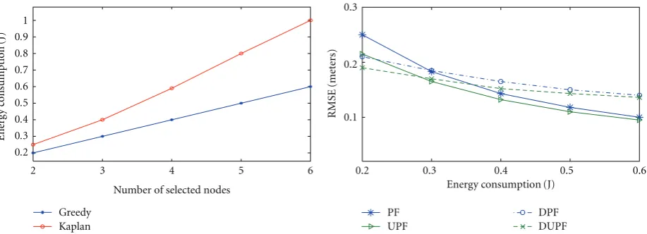
6.4. Energy Consumption. Figure 7 shows the energy con-sumption of node selection algorithms. In Figure 7(a), we compare the energy consumption of the proposed greedy algorithm and Kaplan algorithm as the number of selected nodes increases, using the the residual energy-based metrics defined in (3). Simulation results indicate an increase of the energy consumption with growing number of nodes. We highlight that the rise of the greedy algorithm energy consumption is superlinear using the energy-based metric introduced by Heinzelman in [10] while the rise is linear using our proposed residual energy-based metric. Defini-tively can be concluded that the greedy selection algorithm outperforms the Kaplan selection algorithm to select the sen-sors that would give the most prolonged life to the network. InFigure 7(b), RMSE versus energy consumption of PF, DPF, UPF, and DUPF algorithms using greedy selection has been shown.
In conclusion, the energy consumption increases with the number of active nodes; on the other hand the tracking error decreases as the the number of active nodes increases. A tradeoffbetween the performance and the number of nodes is needed to save energy.
7. Conclusion
function in the cluster. The node selection procedures were integrated into a particle filter and tested on simulated data. The optimal greedy-based algorithm was extended at the real scenario to consider the energy consumption over more measurement intervals. A lower bound was also intro-duced. The experiments indicate that the proposed approach outperforms the existing algorithms in literature. Extensive simulations showed that the target tracking system yields good accuracy for lower velocity of the target. The tracking performances get worse as the noise and the target velocity increase. The bootstrap particle filter and the unscented particle filter for the centralized and distributed scheme and the distributed sigma-point information filter [4] have been implemented and the accuracies have been compared. Furthermore, we have presented a closed-form derivation of PCRB as a performance criterion, eliciting the influence of the number of active nodes, the channel parameters and the model parameters. The formula has been derived and the tracking protocol has been evaluated for linear dynamic’s models and for a nonlinear Gaussian observation’s model. Finally, in this study we assumed an intra-cluster communication and limited ourselves to consider a single cluster in which an even energy consumption by the sensor nodes has been assumed. Future work is investigating the implementation of algorithms to report tracking samples to multiple cluster heads.
Acknowledgement
The author would like to thank Professor Ian Akyildiz for the helpful suggestions.
References
[1] I. F. Akyildiz, W. Su, Y. Sankarasubramaniam, and E. Cayirci, “Wireless sensor networks: a survey,”Computer Networks, vol. 38, pp. 393–422, 2002.
[2] A. T. Ihler, J. W. Fisher III, R. L. Moses, and A. S. Willsky, “Nonparametric belief propagation for self-localization of sensor networks,”IEEE Journal on Selected Areas in Commu-nications, vol. 23, no. 4, pp. 809–819, 2005.
[3] J. Lee, K. Cho, S. Lee, T. Kwon, and Y. Choi, “Distributed and energy-efficient target localization and tracking in wireless sensor netwoks,” Computer Communications, vol. 29, pp. 2494–2505, 2006.
[4] T. Vercauteren and X. Wang, “Decentralized sigma-point information filters for target tracking in collaborative sensor networks,”IEEE Transactions on Signal Processing, vol. 53, no. 8, pp. 2997–3009, 2005.
[5] D. Estrin, R. Govindan, J. Heidemann, and S. Kumar, “Next century challenges: Scalable coordination in sensor networks,” in Proceedings of 5th ACM/IEE International Conference on Mobile Computing and Networking (MobiCom ’99), pp. 263– 270, Seattle, Washington, August 1999.
[6] E. Ertin, J. W. Fisher, and L. C. Potter, “Maximum mutual information principle for dynamic sensor query problems,” inProceedings of the International Workshop on Information Processing in Sensor Networks (IPSN ’03), pp. 405–416, Palo Alto, Calif, USA, April 2003.
[7] H. Wang, G. Pottie, K. Yao, and D. Estrin, “Entropy-based sensor selection heuristic for target localization,” inProceeding of the 3rd International Symposium on Information Processing in Sensor Networks (IPSN ’04), pp. 36–45, Berkeley, Calif, USA, April 2004.
[8] L. M. Kaplan, “Global node selection for localization in a distributed sensor network,”IEEE Transactions on Aerospace and Electronic Systems, vol. 42, no. 1, pp. 113–135, 2006. [9] L. M. Kaplan, “Local node selection for localization in a
distributed sensor network,”IEEE Transactions on Aerospace and Electronic Systems, vol. 42, no. 1, pp. 136–146, 2006. [10] W. B. Heinzelman, A. P. Chandrakasan, and H.
Balakrish-nan, “Energy-Efficient Communication Protocol forWireless Microsensor Networks,” inProceedings of 33rd Hawaii Inter-national Conference on System Sciences (HICSS ’00), Maui, Hawaii, January 2000.
[11] L. Arienzo and M. Longo, “Energy-efficient tracking strategy for wireless sensor networks,” inProceeding of the 5th IEEE International Conference on Mobile Ad-Hoc and Sensor Systems (MASS ’08), pp. 595–602, Atlanta, Ga, USA, September 2008. [12] H. T. Kung and D. Vlah, “Efficient location tracking using
sensor networks,” inProceedings of the IEEE Wireless Commu-nications & Networking Conference (WCNC ’03), March 2003. [13] C.-Y. Lin and Y.-C. Tseng, “Structures for in-network moving object tracking in wireless sensor networks,” in Proceeding of the 1st International Conference on Broadband Networks (BroadNets ’04), pp. 718–727, October 2004.
[14] W. Zhang and G. Cao, “DCTC: dynamic convoy tree-based collaboration for target tracking in sensor networks,” IEEE Transactions on Wireless Communications, vol. 3, no. 5, pp. 1689–1701, 2004.
[15] W. Zhang and G. Cao, “Optimizing tree reconfiguration for mobile target tracking in sensor networks,” inProceedings of the 23rd Annual Joint Conference of the IEEE Computer and Communications Societies (INFOCOM ’04), vol. 4, pp. 2434– 2445, 2004.
[16] Q. Wang, W.-P. Chen, R. Zheng, K. Lee, and L. Sha, “Acoustic target tracking using tiny wireless sensor devices,” inProceedings of the International Workshop on Information Processing in Sensor Networks (IPSN ’03), pp. 642–657, 2003. [17] W.-P. Chen, J. C. Hou, and L. Sha, “Dynamic clustering for
acoustic target tracking in wireless sensor networks,” IEEE Transactions on Mobile Computing, vol. 3, no. 3, pp. 258–271, 2004.
[18] J. Liu, J. Reich, and F. Zhao, “Collaborative in-network processing for target tracking,”EURASIP Journal on Applied Signal Processing, vol. 2003, no. 4, pp. 378–391, 2003. [19] F. Zhao, J. Shin, and J. Reich, “Information-driven dynamic
sensor collaboration for tracking applications,” IEEE Signal Processing Magazine, vol. 19, no. 2, pp. 61–72, 2002.
[20] C. M. Kreucher, A. O. Hero, K. D. Kastella, and M. R. Morelande, “An Information-based approach to sensor man-agement in large dynamic networks,”Proceeding of IEEE, vol. 95, pp. 978–999, 2007.
[21] W. B. Heinzelman, A. P. Chandrakasan, and H. Balakrishnan, “An application-specific protocol architecture for wireless microsensor networks,”IEEE Transactions on Wireless Com-munications, vol. 1, no. 4, pp. 660–670, 2002.
[23] I. Stojmenovic and X. Lin, “Power-aware localized routing in wireless networks,” IEEE Transactions on Parallel and Distributed Systems, vol. 12, no. 11, pp. 1122–1133, 2001. [24] H. Van Trees,Detection, Estimation, and Modulation Theory,
Part I, John Wiley & Sons, New York, NY, USA, 1968. [25] P. Tichavsky, C. H. Muravchik, and A. Nehorai, “Posterior
cram´er-rao bounds for discrete-time nonlinear filtering,”IEEE Transactions on Signal Processing, vol. 46, no. 5, pp. 1386–1396, 1998.
[26] A. Doucet, N. De Freitas, and N. Gordon,Sequential Monte Carlo Methods in Practice, Springer, London, UK, 2001. [27] N. J. Gordon, D. J. Salmond, and A. F. M. Smith, “Novel
approach to nonlinear/non-Gaussian Bayesian state estima-tion,”IEE Proceedings-F, vol. 140, no. 2, pp. 107–113, 1993. [28] M. S. Arulampalam, S. Maskell, N. Gordon, and T. Clapp, “A
tutorial on particle filters for online nonlinear/non-Gaussian Bayesian tracking,”IEEE Transactions on Signal Processing, vol. 50, no. 2, pp. 174–188, 2002.
[29] Y. Bar-Shalom, X. R. Li, and T. Kirubarajan,Estimation with Applications to Tracking and Navigation, John Wiley & Sons, New York, NY, USA, 2001.
[30] A. H. Jazwinski, Stochastic Processes and Filtering Theory, Academic Press, New York, NY, USA, 1970.
[31] R. Van der Merwe, A. Doucet, N. De Freitas, and E. Wan, “The unscented particle filter,” inAdvances in Neural Information Processing Systems, pp. 548–590, 2000.
[32] D. Guo and X. Wang, “Dynamic sensor collaboration via sequential Monte Carlo,” IEEE Journal on Selected Areas in Communications, vol. 22, no. 6, pp. 1037–1047, 2004. [33] C. H. Papadimitriou and K. Steiglitz,Combinatorial
Optimiza-tion: Algorithms and Complexity, Prentice-Hall, Englewood Cliffs, NJ, USA, 1982.
[34] T. A. Feo and M. G. C. Resende, “Greedy randomized adaptive search procedures,”Journal of Global Optimization, vol. 6, no. 2, pp. 109–133, 1995.
[35] W. L. G. Koontz, P. M. Narendra, and K. Fukunaga, “A branch and bound clustering algorithm,”IEEE Transactions on Computers, vol. 24, no. 9, pp. 908–915, 1975.
[36] L. Arienzo, Energy-efficient target tracking through wireless sensor networks. Cross-layer design and optimization, Ph.D. thesis, School of Electrical and Information Engineering, University of Salerno, Salerno, Italy, March 2008.