©
DOI: 10.1534/genetics.103.025692
Stochastic Models for Horizontal Gene Transfer:
Taking a Random Walk Through Tree Space
Marc A. Suchard
1Department of Biomathematics, David Geffen School of Medicine, University of California, Los Angeles, California 90095-1766
Manuscript received December 11, 2003 Accepted for publication February 1, 2005
ABSTRACT
Horizontal gene transfer (HGT) plays a critical role in evolution across all domains of life with important biological and medical implications. I propose a simple class of stochastic models to examine HGT using multiple orthologous gene alignments. The models function in a hierarchical phylogenetic framework. The top level of the hierarchy is based on a random walk process in “tree space” that allows for the development of a joint probabilistic distribution over multiple gene trees and an unknown, but estimable species tree. I consider two general forms of random walks. The first form is derived from the subtree prune and regraft (SPR) operator that mirrors the observed effects that HGT has on inferred trees. The second form is based on walks over complete graphs and offers numerically tractable solutions for an increasing number of taxa. The bottom level of the hierarchy utilizes standard phylogenetic models to reconstruct gene trees given multiple gene alignments conditional on the random walk process. I develop a well-mixing Markov chain Monte Carlo algorithm to fit the models in a Bayesian framework. I demonstrate the flexibility of these stochastic models to test competing ideas about HGT by examining the complexity hypothesis. Using 144 orthologous gene alignments from six prokaryotes previously collected and analyzed, Bayesian model selection finds support for (1) the SPR model over the alternative form, (2) the 16S rRNA reconstruction as the most likely species tree, and (3) increased HGT of operational genes compared to informational genes.
T
RADITIONAL views of molecular evolution hold tween two different prokaryotic species, and (3) trans-that genetic material mutates slowly over time as it duction of genetic material through viruses. Finally, is passed in a vertical fashion from parent to progeny. HGT also has medical importance (Brown 2003). In Molecular phylogenetics then aims to reconstruct this the field of infectious diseases, HGT among bacterial history of inheritance of genetic sequence data from pathogens of antibiotic resistance genes has greatly con-contemporary organisms into a tree-like structure. How- tributed to the emergence of multidrug-resistant bacte-ever, belief in a single tree, mandated by vertical trans- ria in clinical settings (Leverstein-van Hallet al.2002). mission, for all genetic material is changing. Evolution- In the field of oncology, HGT may also affect tumor ary biologists increasingly recognize the horizontal progression;Bergsmedhet al.(2001) show that eukary-transmission of genetic material between distantly re- otic cells can transfer active oncogenes.lated organisms as an important mechanism of evolu- Three general methods have been employed to exam-tion (Syvanen1994;Lawrence1999;Jainet al.2002). ine HGT. The first focuses on single genomes and iden-The process of horizontal (or lateral) gene transfer tifies genes suspected to have been imported through (HGT) plays a critical role across all domains of life HGT by examining variation in nucleotide base compo-and in particular among prokaryotes (Jain et al.1999; sition and codon usage patterns (Lawrenceand
Och-Kooninet al.2001). For example, many prokaryotes are man, 1997). The latter two methods are comparative agile at quickly adapting to new environments. Often, studies across species. One uses similarity approaches this ability stems from the acquisition of new genes based on gene content to identify HGT (Ragan2001) through HGT rather than through random mutation and to propose average genome or species-level trees (Lawrence1999). At least three mechanisms promote (Snelet al.1999), while the alternative method endorses HGT in prokaryotes (Jainet al. 2002). These include: phylogenetic reconstruction using orthologous genes (1) transformation in which free DNA sequences are (Jain et al. 1999). Base composition and codon bias absorbed from the environment, (2) conjugation be- studies may perform poorly when compared to
phyloge-netic methods (Koskiet al.2001). Further, phylogenetic methods offer at least one advantage over similarity-based
1Address for correspondence:Department of Biomathematics, David
approaches. The reconstructed phylogenies have direct Geffen School of Medicine, UCLA, 650 Charles Young Dr., Box 951766,
Los Angeles, CA 90095-1766. E-mail: [email protected] biological interpretability as descriptions of the
ing evolutionary histories of the different genes (Doo- genes. This hypothesis and others can be tested by inte-grating over all possible species trees and gene trees
little1999). If a reconstructed gene tree differs from
the assumed phylogeny of the species being studied, weighed by their posterior probabilities. This Bayesian model-averaging approach reduces the possible bias in-then HGT is offered as a possible explanation (Syvanen
1994). One intrinsic difficulty is that the true species herent in selecting a specific species tree, minimizes underestimation of the uncertainty associated with the tree is often itself unknown. Therefore, it is necessary
to either fix the species tree to equal the inferred gene hypotheses (Taylor et al. 1996), and eliminates the need forad hocanalyses. Formal comparison of different tree for a specially chosen gene,e.g., the 16S rRNA tree
(Woese 2000), or simultaneously estimate the species models for HGT will help gather further insight into the underlying biological processes.
tree and gene trees given a biologically plausible model relating them. As a first step, several research groups have attacked the inverse problem of reconstructing a
MODEL
species tree given gene trees subject to HGT. Most
nota-ble are the parsimony-based reconciled tree work by Within-gene reconstruction model:I begin with a hier-archical framework for phylogenetic reconstruction us-Page and colleagues (e.g.,Page2000) and the
algorith-mic work of Mirkinet al.(2003). ing molecular sequence dataY(Suchardet al.2003a). Data Y ⫽ (Y1, . . . ,YK) consist of Knaturally disjoint I propose a simple class of stochastic models for HGT
that enable the simultaneous estimation of the underly- partitions. Partition dataYkfork⫽1, . . . ,Krepresent the aligned DNA sequences of lengthLkfrom one spe-ing species tree relatspe-ing a group of organisms and the
gene trees subject to HGT for a set of orthologous gene cific gene per partition, sequenced from the same N taxa across all partitions. A hierarchical phylogenetic alignments. These HGT models function in a
hierarchi-cal manner (Suchardet al. 2003a) in which standard model enables the pooling of information across gene partitions to improve estimate precision in individual Bayesian phylogenetic approaches (e.g.,Sinsheimer et
al. 1996; Yang and Rannala 1997; Mau et al. 1999; partitions, while permitting estimation and testing of tendencies in across-partition quantities. For HGT, such
Li et al. 2000; Huelsenbeck et al. 2001) are used to
reconstruct each gene tree from its corresponding gene across-partition quantities include: (1) an overall species tree, (2) appropriate stochastic models from which to alignment. Simultaneous to the reconstructions, the
HGT models impose a second probabilistic distribution construct a probability distribution over individual gene trees given the species tree, and (3) the stochastic model over the gene trees (Maddison1997). This hierarchical
distribution describes the gene trees likelihoods given parameters that may vary between different classes of genes.
an unknown species tree and an unknown number of
HGT events leading from that species tree to each gene To utilize standard Bayesian models for phylogenetic reconstruction (e.g.,Sinsheimer et al.1996;Yangand tree. The model is fit in a Bayesian framework that
naturally handles uncertainty in discrete parameters Rannala 1997;Mau et al.1999; Li et al.2000) within a gene partition, data Yk further divide into ordered such as all the trees and the number of HGT events and
compares various models using Bayes factors (Suchard homologous sitesYk lforl⫽ 1, . . . ,Lk. Site dataYk l⫽ (Yk l1, . . . , Yk l N)t contain one nucleotide from each et al.2001). Stochastic models fit in statistical frameworks
offer several advantages over parsimony approaches. First, taxon, such thatYk l n僆(A, G, C, T) or their ambiguous wildcards forn⫽ 1, . . . ,N. I assume that sites within parsimony may underestimate the number of HGT
events linking the species tree to the gene trees. This a partition are independent and identically distributed, and the likelihood of observing Yk l is given by a consequence is similarly seen in parsimonious
recon-structions of the tree themselves, in which the number multinomial distribution over the 4Npossible outcomes with ambiguous nucleotides being integrated over their of nucleotide substitutions is underestimated. Second,
it is easier in a statistical framework to include measures possible realizations. The multinomial outcome proba-bilities become functions of an unknown tree k that of uncertainty and these levels may be high in the
in-ferred gene trees given the sparse data from which they describes the relatedness of theNtaxa, branch lengths
tk⫽ (tk1, . . . ,tk B), and a model to describe nucleotide are reconstructed.
One additional advantage of building stochastic mod- mutation along these branches, all within partitionk. I elect for a reversible, continuous-time Markov chain els for HGT is the ability to compare competing models
and to incorporate possible differences in the stochastic (CTMC) model for nucleotide substitution (
Felsen-stein 1981) popularized by Tamura and Nei (1993)
processes across genes, while assessing the significance
of these differences in a formal statistical framework. (TN93). The TN93 model is further parameterized by two transition:transversion rate ratios, ␣k between pu-As one example of possible differences across genes,
Jain et al. (1999) propose the complexity hypothesis. rines A and G and␥kbetween pyrimidines C and T, and the stationary distribution of the underlying Markov Under this hypothesis, genes are divided into one of two
classes, informational or operational genes. Between chaink⫽(kA,kG,kC,kT). The final scale parameter in the TN93 model is fixed such that branch lengths classes, the rates of HGT differ. It is suspected that rates
substitu-tions between the nodes inkthat the branch connects. Because I assume a reversible model for nucleotide sub-stitution and make no clock-like restrictions on branch lengths, the root of each tree is unidentifiable ( Felsen-stein1981). As a consequence, the descriptions of all trees to follow are unrooted withN⫺2 internal nodes andB⫽2N ⫺3 branches.
Across-gene hierarchical model:Following the hierar-chical framework of Suchard et al. (2003a), I take branch lengthstkas exponentially distributed with un-known expected divergencek within partitionk and model
⎛ ⎜ ⎜ ⎝
log␣k log␥k logk ⎞ ⎟ ⎟ ⎠
ⵑNormal(V,R)
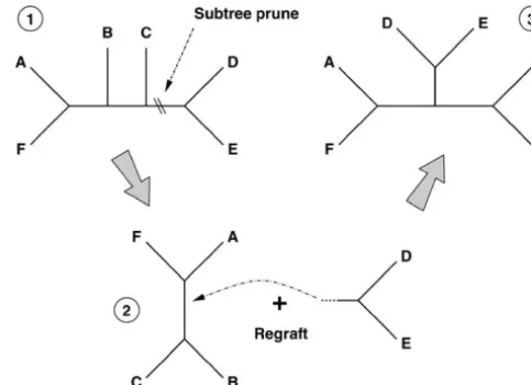
Figure1.—Subtree prune and regraft operator applied to
a six-taxon tree. (1) Operator selects and cuts any branch in the initial tree, pruning away a subtree. (2) Operator regrafts
and
subtree by selecting and subdividing a preexisting branch in the remaining tree. (3) Resultant tree for this realization. kⵑDirichlet(N⌸⫻ ⌸), (1)
whereV ⫽ (A,G,M)tand ⌸⫽ (⌸
A, ⌸G,⌸C,⌸T) are
unknown across-partition-level expectations, variance- called adjacent. Restricting attention to simple graphs in covariance matrix R⫽ diag(2
␣,2␥,2) has diagonal which pairs of vertices may be connected to each other form, and⫺2
␣ ,⫺␥2,⫺2, and N⌸ are unknown across- only by a single edge and no vertex is connected to partition-level measures of precision. LeavingV,R,⌸, itself by a looping edge, a single vertexvfrom graphᏳ andN⌸as unknowns specified only by hyperprior distri- may be adjacent from as few as zero to as many asM⫺ butions and estimating these parameters simultaneously 1 other vertices. The set of all vertices adjacent tovare its with the within-partition-level continuous parameters, neighborhood⌫(v) and the size of this neighborhood
␣k,␥k, andkfor allk, enables the borrowing of strength |⌫(v)|⫽d(v). The specification of a neighborhood for of information from one partition by another, produc- each vertex completes the description ofᏳ, and many
choices are available. ing more precise within-partition-level estimates. I assume
conjugate (when possible) and flat or noninformative Subtree-prune-regraft-based model: One approach to de-fining neighborhoods for each possible tree stems from hyperpriors on these across-partition-level parameters,
as discussed inSuchardet al.(2003a). While the devel- subtree transfer operations (Allen and Steel 2001). Subtree transfer operators act on trees producing local opment of hierarchical priors over the continuous
within-partition-level parameters has been straightforward, rearrangements. Applying a subtree transfer operator to one tree results in the creation of one of several constructing a hierarchical prior over gene treeskthat
incorporates the stochastic nature of HGT is more in- possible new topologies that differs fromby an extent dependent on the operator. The collection of all trees volved. This is illustrated in the next section.
Horizontal gene transfer models:To build a stochas- one operation away from ⫽v becomes its neighbor-hood⌫(v) under that operator. Nearest-neighbor inter-tic model for HGT, I first present a formal description
of the set of all possibleN-taxon trees, commonly re- change (Robinson1971), tree bisection and reconnec-tion (Swofford et al. 1996), and subtree prune and ferred to as “tree space” (Billera et al. 2001), as a
mathematical graph and then discuss several possible regraft (SPR) (Hein 1990, 1993) are three examples. In light of the goals of this article, SPR offers an advan-random walks (D. Aldous and J. Fill, unpublished
results) on this graph that mirror the observed effects tage over the former two operators because of its poten-tial biological interpretation. Applying the SPR operator of HGT.
There exist M ⫽ (2N ⫺ 5)!/2N⫺3(N ⫺ 3)! possible to ⫽ vwith its resultant drawn from⌫
SPR(v) mirrors the differences observed between a species tree and an trees relating N extant taxa (Felsenstein 1981). On
the basis of theseMtrees, I construct a graphᏳ⫽(
, individual gene tree affected by one HGT (or recombi-nation) event (Hein1990, 1993;Jainet al.1999;Allenε
) with vertex set
and edge setε
. Each tree representsa different vertex, or node, in the graph, such that the andSteel 2001).
Figure 1 illustrates one realization of the SPR operator size of the vertex set |
| ⫽ M. An edge uv 僆ε
of agraph describes a direct connection between two of applied to a six-taxon tree. The operator works in two steps. The first step selects and cuts any branch in the the graph’s vertices u, v 僆
. The number of edgesthe same cut branch to a new internal node obtained by subdividing a preexisting branch ininitial⫺ subtree.
Several important properties about the graph ᏳSPR induced by the SPR operator have been previously stud-ied. First, ᏳSPR is regular, implying that every vertexv 僆
SPRpossesses the same degreed(v)⫽2(N⫺3)(2N⫺7) and, hence, neighborhood size (AllenandSteel2001). Also, ᏳSPR is connected, meaning that a sequence of consecutive edges (a path) exists, connecting every pair of vertices in ᏳSPR (Robinson 1971; Allen and Steel2001).
One straightforward stochastic process on any simple graphᏳis an unweighted random walk. A random walk onᏳproceeds from vertex to vertex along existing edges of the graph, generating a discrete-time Markov chain (DTMC), where the states of the chain are the visited vertices. As unweighted, the chain uniform randomly chooses its next vertex to visit from all neighbors of its
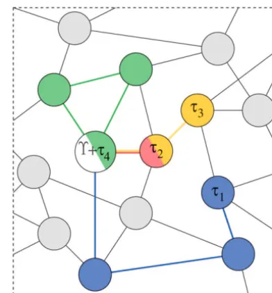
Figure 2.—One possible Markov chain realization on a
current vertex. For this DTMC, the one-event transition
simplified graph for the species tree⌼and four gene trees
probability matrixAhas entries
1, . . . ,4. All chains begin at the same vertex representing
the species tree⌼(in white). The chain producing gene tree
1has lengthE1⫽3 (blue), the chain for2has lengthE2⫽ (A)uv⫽
⎧ ⎭ ⎫ ⎩
1
d(u) if verticesu andvare adjacent or 0 otherwise,
1 (red), the chain for3has lengthE3⫽2 (yellow), and the
chain for4has lengthE4⫽3 (green). Note that this latter (2)
chain returns to its starting state; a parsimony-like analysis
defining the probability ofuchanging intovas a result would estimateE4⫽ 0. Not depicted are chains with actual length zero; these are most probablea priori.
of one random event. It should be noted thatAis just the adjacency matrix of Ᏻ rescaled to be a stochastic matrix [i.e.,兺v(A)uv⫽1].
⌼ⵑ Multinomial(z), (4) On the basis of K random walks on the graph ᏳSPR
induced by the SPR operator, I construct a hierarchical wherez⫽(z1, . . . ,zM) are constants, the prior probabili-prior over the joint distribution of all gene treesk. To ties of the MpossibleN-taxon trees. When little or no accomplish this task, I assume: information is available about⌼, one reasonable choice isz1 ⫽ . . . ⫽ zM ⫽ 1/M; alternately, one may choose An unknown species tree⌼exists.
z such that the prior odds of competing hypotheses The vertex representing⌼is the initial state ofKMarkov
regarding ⌼ are one in a hypothesis-testing setting chains.
(Suchardet al. 2003a). A further choice is discussed The Markov chains are conditionally independent given
later. I further assume a conditionally independent
⌼andA.
prior on allEk, The vertex representingkis the final state of the kth
chain. E
kⵑPoisson(⌳k), (5) And each chain is of unknown length 0ⱕ Ek⬍ ∞.
where ⌳kis the expected number of HGT events for Figure 2 depicts one set of the possible paths ofK⫽ 4
gene kand is a deterministic function of across-gene-Markov chains starting at species tree⌼and ending at
level parameters. This prior is conjugate to (3), allowing gene trees k on a small portion of a representative all E
k to be integrated out of the model, improving graph. The lengths of pathsEkshown range from one sampling efficiency (Liu 1994),
to three. I illustrate no paths of length zero, but these
realizations should be most likely. A parsimony-like anal- q(
k⫽v|⌼ ⫽u,⌳k)⫽
兺
∞Ek⫽0
q(k⫽v|⌼ ⫽u, Ek)q(Ek|⌳k). ysis considering beginning and end points of the chains
in Figure 2 would, for example, underestimate E4 as (6)
zero instead of three.
Lettingq(k⫽v|⌼ ⫽u,⌳k)⫽(P)uv, the multistep transi-Given the assumptions listed above, the probability
tion probability matrix, of species tree⌼giving rise to gene treekafterEkHGT
events is
P ⫽
兺
∞
Ek⫽0
AEkq(Ek|⌳k), q(k⫽v|⌼ ⫽u, Ek)⫽(AEk)uv. (3)
To complete the hierarchical specification, I assign a ⫽
兺
∞ Ek⫽0AEkexp(⫺⌳k)⌳ Ek k
⫽exp(⫺⌳k)exp(⌳kA), 1983). GLMs link the mean response, in this case⌳k, to a set of linear predictors. First, I divide allK genes
⫽exp{⌳k(A⫺ I)}⫽exp(⌳kQ), (7)
into one ofC possible classes, where the definition of whereIis the M⫻ Midentity matrix and Q⫽ P⫺ I
the classes depends on the specific research question is the CTMC infinitesimal rate matrix representation of
at hand. To identify gene-class membership in the GLM, the HGT process. In this parameterization,⌳kare scaled
I construct a K ⫻ C design matrix D ⫽ (Dk c), where as the expected number of HGT events per gene. Let
matrix elementsDk1⫽1 for allk, representing the
base-⌳ ⫽ (⌳1, . . . , ⌳K). Then, recalling the conditional
line multiplier for the reference class, and independence assumption between Markov chains, the
joint distribution over all gene treeskbecomes
Dk c⫽ ⎧ ⎨ ⎩
1 if genek僆classc
0 otherwise, (9)
q(1⫽v1, . . . ,K⫽ vK|⌼ ⫽u,⌳)⫽
兿
Kk⫽1
(P)uvk. (8)
for c ⫽ 2, . . . , C, representing the offset multipliers Calculating the probabilities in (8) requires
numeri-for the remaining classes. Such a design matrix is stan-cal methods to determine the matrix exponential
involv-dard in regression problems involving categorical de-ing PSPR. These methods involve calculating the
com-pendent variables. I model plete set of eigenvalues and eigenvectors of PSPR,
requiringᏻ(M3) operations. Such procedures become
log⌳k⫽
兺
Cc⫽1
cDk c, (10) quickly computationally prohibitive asN, and henceM,
increases. As a consequence, numerical approximations
where linear combinations of predictors⫽(1, . . . , may be necessary to develop weighted graph extensions
C) specify, on the log-scale, the expected number of toᏳSPR directly. The weights in these extended graphs
HGT events for all classes. I complete the hierarchical would be functions of unknown parameters and
sam-prior specification by assuming pling these parameters would necessitate repetitive
diag-onalization. ⵑ Normal(L,⌿). (11)
Random walks with analytic solutions:An alternative to
I setL ⫽(⫺2, 0, . . . , 0) and⌿⫽ diag(10, . . . , 10). this computational barrier involves using random walks
This provides a quite diffuse prior on, with the median on graphs for which analytic solutions are known for
expected number of HGT events per gene⬇0.14 (
Gar-any size M. To help find such solutions, Equation 7
cia-Vallveet al.2000) for all classes. demonstrates the close connection between a DTMC
As an example of how this GLM construction func-with a Poisson-distributed number of events and a CTMC.
tions, consider theC⫽2 classes case. Then, In fact, any such DTMC can be expressed as a unique
CTMC, called the “continuized” version (D. Aldous
andJ. Fill, unpublished results). Analytic solutions for ⌳ k⫽
⎧ ⎨ ⎩
exp(1) if genek僆class 1
exp(1) ⫻exp(2) if genek 僆class 2. (12) several weighted and unweighted CTMC processes on
a complete graph are commonly used in phylogenetics.
When2⫽ 0, no difference across classes exists. Like-In a complete graph, all vertices are adjacent to all
wise, when2⬍0, the expected number of HGT events others. The most notable examples are the CTMC
mod-per gene is smaller in class 2 than in class 1, and when els for nucleotide substitution. The simplest model by
2⬎0, the expected number is larger.
JukesandCantor(1969) is unweighted. In the appen-dix, I present the multistep transition probability matrix
PGJCfor a generalized Jukes-Cantor (GJC) model involv- STATISTICAL FRAMEWORK ing an arbitrary number of vertices M. Proposed by
Comparing the relative appropriateness of the various
Kimura(1980), the next most sophisticated model for
stochastic models for HGT proposed in preceding sec-a complete grsec-aph is weighted. This model presupposes
tions and testing for significant differences in the ex-that the vertices are divided into two disjoint sets,
1傼pected number of HGT events across genes can be
ac-
2⫽
, and that transitions within and between
1andcomplished using Bayesian model selection via Bayes
2 occur at varying rates. In terms of HGT, such afactors. Bayes factors are the Bayesian analog of the weighted random walk may prove useful to model
vary-likelihood-ratio test (LRT), but suffer from fewer diffi-ing rates of HGT between different groups of taxa.
Let-culties than LRTs in discrete spaces, when comparing ting M1 ⫽ |
1|, M2 ⫽ |
2|, and R equal the ratio ofnon-nested models and with sparse data (Suchardet within- to between-transition rates, I present the
al.2001). A Bayes factorB10measures the relative change multistep transition probability matrixPGKgivenM1,M2,
in the support of the dataYin favor of one statistical and R for a generalized Kimura (GK) model in the
modelM1over another modelM0and equals the ratio
appendix.
of the marginal likelihoodm(Y|M1) ofM1over the
mar-Modeling differences across gene classes:I
incorpo-ginal likelihood m(Y|M0) of M0 (Kass and Raftery rate potential differences across genes in the expected
1995). To calculate Bayes factors, frequently more effi-number of HGT events⌳kby employing a generalized
TABLE 1 integrals hidden in the marginal likelihoods directly are
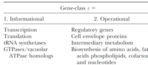
available. Functional definitions of two distinct gene classes,
When models are nested, a relatively simple Bayes adopted fromRiveraet al.(1998) factor calculation is available via the Savage-Dickey ratio
(VerdinelliandWasserman1995) and involves gener- Gene-classc⫽
ating a posterior sample from the larger model only
1. Informational 2. Operational
(Suchardet al.2003b). For example, to assess the
sig-Transcription Regulatory genes
nificance of differences across gene classes in the
ex-Translation Cell envelope proteins
pected number of HGT events, let M1 represent the
tRNA synthetases Intermediary metabolism
unrestricted model proposed above. Nested withinM1
GTPases/vacuolar Biosynthesis of amino acids, fatty
existsM0, the equal-rates model, wherec⫽0 forc ⫽
ATPase homologs acids phospholipids, cofactors,
2, . . . ,C. Further, the GJC model is nested within the and nucleotides GK model, as both are equal whenR⫽1.
On the other hand, the GJC and SPR models are non-nested, but both possess zero free parameters in their
respectivePmatrices. For two arbitrary modelsM0and Bacillus subtilis(Bs), a gram-positive bacterium; Methano-M1 in situations like this, it is possible to estimate the coccus jannaschii(Mj), a methanogen; andArchaeoglobus posterior probabilities p(M0|Y) and p(M1|Y) by con- fulgidus(Af), a thermophilic sulfate-reducing methano-structing a mixture model over the joint space of M0 gen relative. The first four organisms are Eubacteria, andM1. By applying the Bayes theorem, while the last two are Archaea. Jain et al. (1999) con-struct the gene alignments on the basis of amino acid B10⫽
p(M1|Y) p(M0|Y)
冒
q(M1) q(M0)⫽
Posterior odds
Prior odds , (13) translations, assuming a star tree to reduce alignment bias (Lake 1991), and classify each gene into one of two distinct classes, informational and operational genes where q(M0) and q(M1) are the prior probabilities of
(Riveraet al.1998). Table 1 lists the functional charac-modelsM0andM1in the mixture. Generally, I assume
teristics of the genes that fall into each class. As a gener-equal prior probabilities, q(M0) ⫽ q(M1) ⫽ 1⁄2, when
alization, informational gene products interact in large reporting posterior estimates. However, improved
effi-complex systems; this is especially true of the transla-ciency in estimating B10 can be garnered by adjusting
tional and transcriptional apparatuses. On the other these prior probabilities such that p(M0|Y)⬇ p(M1|Y)
hand, most operational gene products function inde-(CarlinandChib1995;Suchardet al.2002).
pendently or in small protein assemblies. In total,Jain
Models SPR and GK neither are nested nor contain
et al.(1999) assign 56 genes as informational and 88 as the same number of free parameters. One might
enter-operational, employ these genes to examine the com-tain constructing a reversible-jump Markov chain Monte
plexity hypothesis, and find support for higher levels of Carlo (MCMC) sampler (Green 1995) over the joint
HGT among the operational genes as compared to the space of these models to compute the Bayes factor in
informational genes. support of SPR over GK. However, a simpler algebraic
I parallel the above analysis by assuming that the solution exists given the two preceding Bayes factor
number of the different gene classesC ⫽2. I let class calculations,
c ⫽1 represent the informational genes and classc ⫽ 2 represent the operational genes. To further maintain BSPR,GK⫽
BSPR,GJC BGJC,GK
. (14)
consistency withJainet al.(1999), I exclude third codon position nucleotides from all alignments and assume To estimate all model parameters and Bayes factors, I
that first and second codon position nucleotides are employ MCMC. I further develop this MCMC algorithm
evolving independently under the same process for each and discuss its performance in theappendix.
gene.
Selection of stochastic model:I begin by comparing
EXAMPLE the relative likelihoods of the three different stochastic
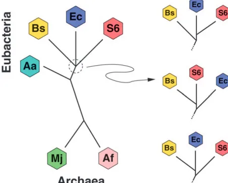
models, SPR, GJC, and GK. For the GK model, I define To illustrate these stochastic models for HGT and
my two disjoint sets of trees as (1) those that support a methods to test hypotheses about them, I examine a
split between the four Eubacteria and the two Archaea, large set of orthologous, prokaryotic genes collected by
1, and (2) those that do not,
2. These definitionsJainet al.(1999). The data consist ofK⫽144 separate
offer a first approximation to modeling differing rates gene alignments. Each alignment contains orthologous
of HGT within life domains and across domains in this copies of a single gene from six prokaryotes. These
example. HGT events that start and end in set
1 are prokaryotes are:Aquifex aeolicus(Aa), an early branchingwithin domain transfers, while events that start in
1 thermophilic eubacterium; Escherichia coli (Ec), aform two distinct clades (Feng et al. 1997) and Aa is the earliest branching species of the Eubacteria studied (Deckertet al.1998). The branching order of the re-maining three Eubacteria Ec, S6, and Bs is more ambigu-ous (Giovannoniet al.1996). The three possible resolu-tions of this trifurcation are depicted on the right side of Figure 3. Much of the debate surrounding the trifur-cation depends on data choice and reconstruction methodology. For example, the top resolution produces species tree⌼Ec-S6that places Ec and S6 as nearest neigh-bors. Protein synthesis elongation factor (EF) Tu gene reconstructions support this tree (Lake and Rivera
1996) andJainet al.(1999) fix⌼Ec-S6as their reference tree in their analysis. Reconstructions of 16S rRNA phy-logeny support the middle resolution of species tree
⌼Bs-S6(Coleet al.2003) with Bs and S6 as nearest neigh-bors. The final resolution of species tree ⌼Ec-Bs gains
Figure 3.—Species tree relating six prokaryotes. Species
support from reconstructions of phenylalanyl-tRNA
syn-are:Aquifex aeolicus(Aa),Escherichia coli(Ec),Synechocystis 6803
thetase (TeichmannandMitchison 1999). However,
(S6),Bacillus subtilis(Bs),Methanococcus jannaschii(Mj), and
Archaeoglobus fulgidus(Af). Branch order of three Eubacteria even these three critical genes are subject to HGT (Wolf
Ec, S6, and Bs is under debate, leading to three possible et al. 1999; Zap et al. 1999; Ke et al. 2000) and their
subtrees (shown on right). reconstructed phylogenies may inaccurately represent
the true species tree.
On the basis of the SPR model for HGT, I infer⌼Bs-S6 The log10Bayes factor in favor of SPR over GJC and as the most likely species tree with ⬎0.999 posterior the log10Bayes factor in favor of GK over GJC are probability. The two other resolutions,⌼
Ec-Bsand⌼Ec-S6, are the second and third most likely species trees, re-log10BSPR,GJC⫽19.2 and log10BGK,GJC⫽5.7. (15)
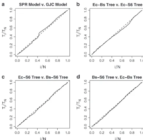
spectively. To estimate the Bayes factors in favor of⌼Bs-S6 Figure 4a illustrates the scaled regeneration quantile against⌼Ec-Bsand⌼Ec-S6, I judiciously reweight my prior (SRQ) plot for estimating the relative posterior proba- probabilities on treeszand calculate
bilities used to calculate log10 BSPR,GJC. No substantial
log10BBs-S6,Ec-Bs⫽7.3 and log10BEc-Bs,Ec-S6⫽5.9. (17) deviation from the slope ⫽ 1 line implies the MCMC
chain is mixing sufficiently to generate this estimate. Similar to the back calculation completed in previous Combining the results in (15), I calculate the log10Bayes section, I estimate
factor in favor of SPR over GK as
log10BBs-S6,Ec-S6⫽ 7.3⫹5.9 ⫽13.2, (18) log10BSPR,GK⫽ 19.2⫺5.7 ⫽13.5. (16)
while direct calculation of log10BBs-S6,Ec-S6using the sam-pler yields approximately the same result. Figure 4, b–d, Considering these Bayes factor estimates, the data
strongly reject (KassandRaftery1995) the two com- depicts the SRQ plots relevant to these Bayes factor calculations. Again, the MCMC chain appears well mix-plete graph models with analytic solutions in favor of
the more biologically plausible process based on the ing. Although the posterior support for ⌼Ec-Bsand⌼Ec-S6 initially appears quite small, on a relative scale it is not; SPR operator. However, the GJC and GK models should
not be discounted completely; their computational com- probabilities for the remaining 102 trees are⬎15 orders of magnitude smaller.
plexity does not increase with increasing number of taxa
Nand they can offer some insight into the underlying Data sets as large as theK⫽144 gene alignments from
Jainet al.(1999) are currently rare. Consequentially, I biological processes. For example, the Bayes factor in
favor of GK over GJC offers some indirect support for examine via simulation the number of alignments neces-sary to identify the species tree under the SPR model. differing HGT rates within domains rather than across
domains. One caveat should be kept in mind to keep Under this simulation, I randomly sample without re-placement a fixed number of gene alignmentsK and from drawing too strong a conclusion from this
find-ing—the unbalanced study design with only two Arch- then estimate the posterior support for⌼Bs-S6, assuming this is the true species-tree. I repeat this simulation 20 aea precludes identifying HGT events within that
do-main. All further results in this article are based on the times for each value of K. For K ⫽ 2, the expected posterior probability of ⌼Bs-S6 ⫽ 0.14. This estimate is SPR model.
Estimating the species tree:Figure 3 displays the cur- approaching its prior value, signifying appropriate MCMC sampling with limited data. ApproximatelyK⫽ rently accepted species tree relating the six prokaryotes
As seen from Table 2, the average transition:transver-sion ratio for purines A⬘ is significantly different from the ratio for pyrimidinesG⬘, as the ratios’ 95% Bayesian credible intervals (BCIs) do not overlap, and both ratios are greater than one. This supports the use of the TN93 model for nucleotide substitution over a more restricted model. Estimates of A, G, and⌸ are consistent with a previous study using a subset of the data in a hierarchical framework (Suchardet al.2003a). Also in comparison to this previous study, differences in estimates of M,
2A,2G,2
M, andN⌸all trend in the correct directions given the increase in the number of taxa and genes fit here.
Varying rates of HGT across gene classes: Figure 5 displays model estimates for the linear predictors1and
2 and for the expected number of HGT events per gene,⌳k, for the informational and operational gene classes. The two top plots display histograms of the pos-terior samples of 1 (left) and 2 (right). These plots also include normal approximations to the posterior (solid lines) and prior densities (dashed lines).
Examin-Figure 4.—Scaled regeneration quantile (SRQ) plots to
assess MCMC sampler performance when estimating four rela- ing the plot on the right, the prior density at 2 ⫽ 0
tive posterior probabilities. Plot a was generated when compar- (dotted vertical line) is considerably higher than the
ing the SPR and GJC stochastic models. Plots b–d were gener- normal approximation to the posterior density. Further,
ated when comparing the three most probable species trees.
the 95% BCI of 2 ⫽ (0.27–1.15) and does not cover
No substantial deviation in the slopes from 1 (dashed lines)
zero. Both observations support the hypothesis that2⬆
implies that the chains are mixing well enough to produce
stable estimates. 0 and, hence, that rates of HGT differ between
informa-tional and operainforma-tional genes. Formally, the Bayes factor in favor of differing rates is given by the Savage-Dickey posterior probability ⱖ0.80 and K ⫽ 70 are required
ratio. The log10Bayes factor, forⱖ0.90.
Hierarchical estimates of evolutionary pressures:Ta- log10B⬆
rates,⫽rates⫽ 0.9, (20) ble 2 presents the posterior estimates of the
across-gene-offers substantial support (KassandRaftery1995) in level parameters used to pool information about (␣k,
favor of differing rates.
␥k,k,k). The table also lists posterior estimates of
The bottom plot in Figure 5 transforms 1 and 2 A⬘ ⫽ exp(A⫹1⁄22A),
into the expected number of HGT events per gene and displays histograms of the posterior samples of these G⬘ ⫽ exp(G⫹1⁄22G),
quantities. Depicted in dark shading is⌳kfor the opera-M⬘ ⫽ exp(M⫹1⁄22M). (19)
tional genes and depicted in light shading is⌳kfor the informational genes. Although⌳kfor operational genes These transformed variables report the across-gene-level
is significantly greater than⌳kfor informational genes averages of the two transition:transversion ratios and
expected divergence on their usual, instead of log, scale. from the argument above, a small amount of overlap is
TABLE 2
Hierarchical across-gene-level estimates of evolutionary pressures
Log-scale central tendencies Natural-scale central tendencies Measures of precision
Parameter Mean (95% BCI) Parameter Mean (95% BCI) Parameter Mean (95% BCI)
A 0.48 (0.4–0.52) A⬘ 1.65 (1.59–1.71) 1/2
A 26.59 (20.29–33.77)
G 0.23 (0.180–0.28) G⬘ 1.29 (1.23–1.35) 1/2
G 20.28 (14.67–27.15)
M ⫺1.67 (⫺1.74–⫺1.60) M⬘ 0.19 (0.18–0.21) 1/2
M 17.02 (11.65–23.93)
⌸A 0.35 (0.35–0.35) N⌸ 542.66 (455.47–639.81)
⌸G 0.30 (0.29–0.30)
⌸C 0.17 (0.16–0.17)
⌸T 0.19 (0.18–0.19)
observed (solid shading) between these marginal histo-grams. This overlap results from the high negative corre-lation between1and2(data not shown) and illustrates the need for caution in making inference on the basis of marginal posterior summaries alone.
REMARKS
In this article, I proposed a simple class of stochastic models for HGT. The models are based on a random walk process in tree space and allow for the development of a joint distribution over multiple gene trees given an unknown species tree. I consider two general forms of random walks. The first stems from subtree transfer operations, in particular the SPR operator that mirrors the observed effects that HGT has on an inferred tree. The second form is based on walks over complete graphs and offers numerically tractable solutions for increasing number of taxa. I fit these models using a Bayesian framework to data from six prokaryotes. I find strongest
Figure5.—Analysis of the complexity hypothesis. The top
support for the species tree that places Bs and S6 as two plots depict the posterior distributions of linear predictors nearest neighbors. This tree is supported by 16S rRNA 1and2using histograms and normal approximations (solid reconstructions, but differs from the EF-Tu tree as- lines). Also shown are the predictors’ prior densities (dashed lines). Greater prior than posterior density at2⫽0 (dotted sumed byJainet al.(1999). I demonstrate the flexibility
line) supports a difference in HGT rates between gene classes.
of these stochastic models to test competing ideas about
The bottom plot depicts the posterior distributions of the
HGT by examining the complexity hypothesis and find expected number of HGT events per gene for informational support for increased HGT of operational genes com- genes (light shading) and operational genes (dark shading). pared to informational genes. This latter finding
re-mains unchanged if I fix the species tree to equal the
EF-Tu tree (data not shown). due to sparse phylogenetic data, evolutionary model misspecification, and parallel/convergent evolution can The specific stochastic models for HGT developed in
this article have important limitations. First and fore- falsely produce incongruence between trees (Caoet al. 1998). These effects should upwardly bias the inferred most, the random walks explore only the discrete,
topo-logical portion of tree space and do not consider number of HGT events. However, I suspect this bias is less than one HGT event per gene as only a modest changes in branch lengths between trees as part of the
underlying HGT process. As a result, HGT between percentage of genes should be affected and the error should produce just minor changes in the inferred tree. nearest neighbors in a tree remains unidentified as this
process does not result in a change in the topological There is noa priorireason to suspect that this bias differs between the informational and operational gene classes; configuration of the tree. Model extensions that
con-sider a continuous random drift process on the joint so the bias does not affect the relative difference be-tween classes in HGT rates and inference regarding the space of (,t) (Billeraet al.2001) may circumvent this
shortfall. For a related problem involving coalescence, complexity hypothesis.
For the SPR model, numerical approximations to the
Yang(2002) shows that including branch lengthstinto
the probabilistic model across loci improves power. Ad- matrix exponentials involving the multistep transition probability matrixPSPR may offer promise in handling ditionally, I assume that theKDTMCs representing the
random walks of the gene treeskaway from the species research problems with larger numbers of taxaN(Moler andVan Loan2003). AsNincreases, the square dimen-tree⌼are conditionally independent given⌼. This
as-sumption implies that the evolutionary histories of all sions of PSPR grow superexponential, while the size of the neighborhood of each vertex grows only asᏻ(N2). genes are unlinked, while evidence for the HGT of, at
a minimum, complete operons abounds in prokaryotes As a consequence,PSPRbecomes increasingly sparse. In this situation, the number of unique eigenvalues in-(Kooninet al.2001). Possible modeling aspects include
allowing for linked or partially linked genes. creases substantially slower than the matrix’s dimension. Krylov subspace techniques (SidjeandStewart1999) HGT is not the only process that may cause
incongru-ence between gene trees. Although the effects of lineage may stretch computational limits upward to N ⫽ 8 or more.
sorting should be minor given the extensive divergence
between the species studied here, the inclusion of para- In spite of these limitations, these stochastic models for HGT offer several advantages over previous ap-logous genes copies within the orthoap-logous alignments
Gelman, A., G. RobertsandW. Gilks, 1996 Efficient Metropolis gene alignments. Under these stochastic models, the
jumping rules, pp. 599–608 inBayesian Statistics, Vol. 5, edited species tree is an unknown parameter that may be either by J. Bernardo, J.Berger, A. Dawidand A. Smith. Oxford
University Press, Oxford. integrated out of the analysis as a nuisance parameter
Giovannoni, S., M. Rapp, D. Gordon, E. Urbach, M. Suzukiet al., or estimated jointly with the multiple gene trees. Joint
1996 Ribosomal RNA and the evolultion of bacterial diversity, analysis decreases the possibility of bias introduced pp. 63–85 inEvolution of Microbial Life, edited by D.Roberts, P.
Sharp, G. Alderson and M. Collins. Cambridge University through fixing the species tree when knowledge about
Press, Cambridge, UK. it is uncertain. A stochastic approach also overcomes
Green, P., 1995 Reversible jump Markov chain Monte Carlo compu-the bias inherent in parsimony-like estimation. Furcompu-ther, tation and Bayesian model determination. Biometrika82:711–
732. the hierarchical framework in which the stochastic
Hein, J., 1990 Reconstructing evolution of sequences subjects to model sits enables the borrowing of strength in the
recombination using parsimony. Math. Biosci.98:185–200. estimation of all gene-partition-level estimates including Hein, J., 1993 A heuristic method to reconstruct the history of
se-quences subject to recombination. J. Mol. Evol.36:396–405. the gene trees themselves. Finally, and most
impor-Huelsenbeck, J., F. Ronquist, R. NielsenandJ. Bollback, 2001 tantly, stochastic models lend themselves well to formal
Bayesian inference of phylogeny and its impact on evolutionary statistical testing, with no need for ad hocprocedures. biology. Science294:2310–2314.
Jain, R., M. Rivera and J.Lake, 1999 Horizontal gene transfer The ability to compare differing models for HGT will
among genomes: the complexity hypothesis. Proc. Natl. Acad. continue to shed further insight into the underlying
Sci. USA96: 3801–3806.
biological process. Jain, R., M. Rivera, J. MooreandJ. Lake, 2002 Horizontal gene transfer in microbial genome evolution. Theor. Popul. Biol.61:
I thank the Lake lab, in particular Jon Moore and Jim Lake, for
489–495. stimulating my interest in HGT, for many provocative discussions,
Jukes, T., andC. Cantor, 1969 Evolution of protein molecules, pp. and for providing the SPR adjacency matrices and prokaryote se- 21–132 inMammaliam Protein Metabolism, edited by H.Munro. quences used in this study. I also thank John Huelsenbeck for his Academic Press, New York.
insights into HGT and Janet Sinsheimer and Vladimir Minin for com- Kass, R., andA. Raftery, 1995 Bayes factors. J. Am. Stat. Assoc.90: menting on this manuscript. Fred Fox and the National Science Foun- 773–795.
Ke, D., M. Boissinot, A. Huletsky, F. Picard, J. Frenetteet al., 2000 dation grant 9987641-sponsored University of California, Los Angeles,
Evidence for horizontal gene transfer in evolution of elongation Training Program in Bioinformatics graciously made possible the
factor Tu in enterococci. J. Bacteriol.182:6913–6920. computing facilities to fit all 144 alignments simultaneously. The
com-Kimura, M., 1980 A simple model for estimating evolutionary rates plete data set is available to interested readers at http://www.bio
of base substitutions through comparative studies of nucleotide math.medsch.ucla.edu/msuchard/datasets.html. I am supported in
sequences. J. Mol. Evol.16:111–120.
part by National Institutes of Health grants GM08042 and GM068955 Koonin, E., K. MakarovaandL. Aravind, 2001 Horizontal gene and U.S. Public Health Service grant CA16042. transfer in prokaryotes: quantification and classification. Annu.
Rev. Microbiol.55:709–742.
Koski, L., R. MortonandG. Golding, 2001 Codon bias and base composition are poor indicators of horizontally transferred genes. Mol. Biol. Evol.18:404–412.
LITERATURE CITED
Lake, J., 1991 The order of sequence alignment can bias the
selec-Allen, B., andM. Steel, 2001 Subtree transfer operations and their tion of tree topology. Mol. Biol. Evol.8:378–385.
induced matrices on evolutionary trees. Ann. Combinatorics5: Lake, J., andM. Rivera, 1996 The prokaryotic ancestry of
eukary-1–15. otes, pp. 87–108 inEvolution of Microbial Life, edited by D.
Rob-Bergsmedh, A., A. Szeles, M. Henriksson, A. Bratt, M. Folkman erts, P.Sharp, G.Aldersonand M.Collins. Cambridge Univer-et al., 2001 Horizontal transfer of oncogenes by uptake of apo- sity Press, Cambridge, UK.
ptotic bodies. Proc. Natl. Acad. Sci. USA98:6407–6411. Lawrence, J., 1999 Gene transfer, speciation and the evolution of
Billera, L., S. HolmesandK. Vogtmann, 2001 Geometry of the bacterial genomes. Curr. Opin. Microbiol.2:519–523. space of phylogenetic trees. Adv. Appl. Math.27:733–767. Lawrence, J., andH. Ochman, 1997 Amelioration of bacterial
ge-Brown, J., 2003 Ancient horizontal gene transfer. Nat. Rev. Genet. nomes: rates of change and exchange. J. Mol. Evol.44:383–397.
4:121–132. Leverstein-van Hall, M., A. Box, H. Blok, A. Pauuw, A. Fluitet
Cao, Y., A. Janke, P. Waddell, M. Westerman, O. Takenaka et al., 2002 Evidence of extensive interspecies transfer of integron-al., 1998 Conflict among individual mitochondrial proteins in mediated antimicrobial resistance genes among multidrug-resis-resolving the phylogeny of Eutherian orders. J. Mol. Evol.47: tant Enterobacteriaceae in a clinical setting. J. Infect. Dis.186:
307–322. 49–56.
Carlin, B., andS. Chib, 1995 Bayesian model choice via Markov Li, S., D. PearlandH. Doss, 2000 Phylogenetic tree construction chain Monte Carlo methods. J. R. Stat. Soc. Ser. B57:473–484. using Markov chain Monte Carlo. J. Am. Stat. Assoc.95:493–508.
Cole, J., B. Chai, T. Marsh, R. Farris, Q. Wanget al., 2003 The Liu, J., 1994 The collasped Gibbs sampler in Bayesian computations ribosomal database project (RDP-II): previewing a new auto- with applications to a gene regulation problem. J. Am. Stat. Assoc. aligner that allows regular updates and the new prokaryotic taxon- 89:958–966.
omy. Nucleic Acids Res.31:442–443. Maddison, W., 1997 Gene trees in species trees. Syst. Biol.46:523–
Deckert, G., P. Warren, T. Gaasterland, W. Young, A. Lenox 536.
et al., 1998 The complete genome of the hyperthermophilic Mau, B., M. NewtonandB. Larget, 1999 Bayesian phylogenetic bacteriumaquifex aeoclicus.Nature392:353–358. inference via Markov chain Monte Carlo methods. Biometrics
Doolittle, W., 1999 Lateral gene transfer, genome surveys and the 55:1–12.
phylogeny of prokaryotes. Science286:1443a. McCullagh, P., andJ. Nelder, 1983 Generalized Linear Models: Mono-Felsenstein, J., 1981 Evolutionary trees from DNA sequences: a graphs on Statistics and Applied Probability. Chapman & Hall, New
maximum likelihood approach. J. Mol. Evol.17:368–376. York..
Feng, D., G. ChoandR. Doolittle, 1997 Determining divergence Mirkin, B., T. Fenner, M. GalperinandE. Koonin, 2003 Algo-times with a protein clock: update and reevaluation. Proc. Natl. rithms for computing parsimonious evolutionary scenarios for Acad. Sci. USA94:13028–13033. genome evolution, the last universal common ancestor and
domi-Garcia-Vallve, S., A. RomeuandJ. Palau, 2000 Horizontal gene nance of horizontal gene transfer in the evolution of prokaryotes. transfer in bacterial and archeal complete genomes. Genome BMC Evol. Biol.3:2.
pute the exponential of a matrix, twenty-five years later. Soc. Ind. branch length restrictions in a Bayesian framework. Syst. Biol.
52:48–54. Appl. Math. Rev.45:3–49.
Mykland, P., L. TierneyandB. Yu, 1995 Regeneration in Markov Swofford, D., G. Olsen, P. WaddellandD. Hillis, 1996 Phyloge-netic inferences, pp. 407–514 inMolecular Systematics, Ed. 2, edited chain samplers. J. Am. Stat. Assoc.90:233–241.
Page, R., 2000 Extracting species trees from complex gene trees: by D.Hillis, C.Moritzand B.Mable. Sinauer Associates, Sun-derland, MA.
reconciled trees and vertebrate phylogeny. Mol. Phylogenet. Evol.
14:89–106. Syvanen, M., 1994 Horizontal gene transfer: evidence and possible consequences. Annu. Rev. Genet.28:237–261.
Ragan, M., 2001 Detection of lateral gene transfer among microbial
genomes. Curr. Opin. Genet. Dev.11:620–626. Tamura, K., andM. Nei, 1993 Estimation of the number of nucleo-tide substitutions in the control region of mitochondrial DNA
Rivera, M., R. Jain, J. MooreandJ. Lake, 1998 Genomic evidence
of two functionally distinct gene classes. Proc. Natl. Acad. Sci. in humans and chimpanzees. Mol. Biol. Evol.10:512–526.
Taylor, J., A. SiqueiraandR. Weiss, 1996 The cost of adding USA95:6239–6244.
Roberts, G., and S. Sahu, 1997 Updating schemes, correlation parameters to a model. J. R. Soc. Stat. Ser. B58:593–607.
Teichmann, S., andG. Mitchison, 1999 Is there a phylogenetic structure, blocking and parameterization of the Gibbs sampler.
J. R. Stat. Soc. Ser. B59:291–317. signal in prokaryote proteins? J. Mol. Evol.49:98–107.
Verdinelli, I., andL. Wasserman, 1995 Computing Bayes factors
Robinson, D., 1971 Comparison of labeled trees with valency three.
J. Comb. Theor. Ser. B11:105–119. using a generalization of the Savage-Dickey density ratio. J. Am. Stat. Assoc.90:614–618.
Sidje, R., andW. Stewart, 1999 A numerical study of large sparse
matrix exponentials arising in Markov chains. Comput. Stat. Data Woese, C., 2000 Interpreting the universal phylogenetic tree. Proc. Natl. Acad. Sci. USA97:8392–8396.
Anal.29:345–368.
Sinsheimer, J., J. LakeandR. Little, 1996 Bayesian hypothesis Wolf, Y., L. Aravind, N. GrishinandE. Koonin, 1999 Evolution of aminoacyl-tRNA synthetases—analysis of unique domain archi-testing of four-taxon topologies using molecular sequence data.
Biometrics52:193–210. tectures and phylogenetic trees reveals a complex history of hori-zontal gene transfer events. Genome Res.9:689–710.
Snel, B., P. BorkandM. Huynen, 1999 Genome phylogeny based
on gene content. Nat. Genet.21:108–110. Yang, Z., 2002 Likelihood and Bayes estimation of ancestral
popula-Suchard, M., R. WeissandJ. Sinsheimer, 2001 Bayesian selection tion sizes in hominoids using data from multiple loci. Genetics of continuous-time Markov chain evolutionary models. Mol. Biol. 162:1811–1823.
Evol.18:1001–1013. Yang, Z., andB. Rannala, 1997 Bayesian phylogenetic inference
Suchard, M., R. Weiss, K. DormanandJ. Sinsheimer, 2002 Oh using DNA sequences: a Markov chain Monte Carlo method. brother, where art thou? A Bayes factor test for recombination Mol. Biol. Evol.14:717–724.
with uncertain heritage. Syst. Biol.51:715–728. Zap, W., Z. ZhangandY. Wang, 1999 Distinct types of rRNA operons
Suchard, M., C. Kitchen, J. SinsheimerandR. Weiss, 2003a Hier- exist in the genome of the actinomycetethermomonospora chromo-archical phylogeneic models for analyzing multipartite sequence genaand evidence for horizontal gene transfer of an entire rRNA data. Syst. Biol.52:649–664. operon. J. Bacteriol.181:5201–5209.
Suchard, M., R. WeissandJ. Sinsheimer, 2003b Testing a
molecu-lar clock without an outgroup: derivations of induced priors on Communicating editor: J.Hein
APPENDIX
Complete models: To determine the multistep transition probability matrixPGJC for the GJC model withMⱖ 2 states, I first recall that
PGJC⫽ exp(⌳kQGJC) (A1)
is generated from an unweighted complete graph. As a complete graph, it is trivially connected and, therefore, has a unique stationary distribution. This distribution is (1/M, . . . , 1/M).
To determine the eigenvalues ofQGJC, I write
QGJC⫽ 1 M⫺1J⫺
M
M⫺ 1I, (A2)
whereQGJC is scaled such that⌳kis expressed in terms of the expected number of HGT events per gene, Jis the M ⫻ M matrix of all ones, and I is theM ⫻ M identity matrix. MatrixJ has a rank of one and, therefore, one nonzero eigenvalue that equalsM/(M⫺ 1). Given the eigenvalues ofJand expression (A2), theMeigenvalues of
QGJCbecome
冢
0, ⫺M M⫺ 1, . . . ,⫺M
M⫺1
冣
. (A3)Like the standard Jukes-Cantor model, whereM ⫽ 4, the GJC model for anyM ⱖ 2 continues to have only two distinct eigenvalues. Conceptually this results because the qualitative behavior of the underlying Markov chain does not change as the size of the state-space increases.
(PGJC)uv⫽ ⎧ ⎪ ⎨ ⎪ ⎩ 1
M⫹
M⫺1 M exp(⫺
M
M⫺1⌳k) ifu⫽v 1
M⫺
1 Mexp(⫺
M
M⫺1⌳k) otherwise. (A4)
The state-space of the GK model is partitioned into two disjoint sets
1 and
2. Let M1 ⫽ |
1| and M2⫽ |
2|, where M1 ⫹ M2 ⫽ M, and letR be the ratio of rates for transitions within a structural set to transitions between sets. Then, following arguments similar to those above, one can find the multistep transition probability matrixPGK for the GK model.Ifu僆
1, then(PGK)uv⫽ ⎧ ⎪ ⎪ ⎭ ⎫ ⎪ ⎪ ⎩ 1
M⫹
M1⫺ 1 M1
exp(⫺φ1␥⌳k)⫹ M2 M1M
exp(⫺φ2␥⌳k) ifu⫽ v
1
M⫺
1 M1
exp(⫺φ1␥⌳k)⫹ M2 M1M
exp(⫺φ2␥⌳k) else if v僆
11
M⫺
1
Mexp(⫺φ2␥⌳k) otherwise, (A5)
where
␥ ⫽ M
[M1(M1⫺1) ⫹M2(M2⫺ 1)]R⫹2M1M2 ,
φ1⫽M1R⫹M2,
φ2⫽M. (A6)
By symmetry, ifu 僆
2, then(PGK)uv⫽ ⎧ ⎪ ⎪ ⎭ ⎫ ⎪ ⎪ ⎩ 1
M⫹
M2⫺ 1 M2
exp(⫺φ3␥⌳k)⫹ M1 M2M
exp(⫺φ2␥⌳k) ifu⫽ v
1
M⫺
1 M2
exp(⫺φ3␥⌳k)⫹ M1 M2M
exp(⫺φ2␥⌳k) else if v僆
21
M⫺
1
Mexp(⫺φ2␥⌳k) otherwise, (A7)
where φ3⫽ M2R⫹M1. ForR⬆ 1, note that there are four unique eigenvalues whenM1 ⬆ M2and three unique eigenvalues otherwise. This is consistent with the standard Kimura model, in whichM1⫽M2⫽2 with three unique eigenvalues.
Sampling algorithm:For each gene-partitionk, letk⫽ (k,tk,␣k,␥k,k,k) and, then, assemble⫽(1, . . . ,
K) to be the collection of all gene-level parameters. To specify the hierarchical prior parameters, letφ⫽(V,R,⌸, N⌸,⌼,). Across-gene-level parametersφalso includeRwhen considering the GK model and mixing parameter
僆 {0, 1} when comparing models SPR and GJC. I employ a MCMC approach to sample from each model’s joint posterior distribution,p(,φ|Y). I generate samples from these posteriors using two nested Metropolis-within-Gibbs cycles, as laid out inSuchardet al.(2003a) for hierarchical phylogenetic models. The outer cycle first iterates over gene partitions kand then over the parameters inφ. Within each gene partitionk, the inner cycle proceeds over the parameters ink. With the exception of proposals for⌼,,R, and, all parameter proposals follow those in
Suchardet al. (2003a).
The multinomial prior placed on⌼is conjugate to its sampling density. As a result, it is possible to Gibbs sample
⌼from its full conditional distribution for moderately smallM. This full conditional distribution remains multinomial with Mstate probabilities given by
p(⌼ ⫽u|Y,⍀⫺⌼)⫽
兿
K
k⫽1(P)uvkzu
兺
w僆兿
Kk⫽1(P)wvkzw, (A8)
wherek⫽vkfor allkand⍀⫺⌼is the vector of all model parameters (,φ) excluding⌼. Similar to the reweighted prior approach to estimate , varying z can improve sampling efficiency when estimating the relative posterior probabilities of specific species trees⌼.
new parameter values by generating a normal random variate centered at the current value ofR with a tunable variance s2R. Given the high degree of correlation between column vectors in the design matrix D, I expect the posterior distribution ofto also exhibit strong correlation. This expectation stems from a normal linear regression approximation top(exp()|⌳) that has a variance-covariance structure proportional to (DⴕD)⫺1. As a consequence, component-by-component updating of c in should lead to a slowly mixing MCMC chain (Robertsand Sahu 1997). To help ensure adequate mixing, I propose allcsimultaneously using a multivariate normal random variate centered at the current value ofwith a tunable variance-covariance matrix diag(s2
1, . . . ,s
2
C)⌶. I adjust the
tun-able variances such that proposals have acceptance rates of 30–40% (Gelman et al.1996) and fix the correlation matrix⌶approximately equal to the posterior correlation ofdetermined by a trial chain.
When comparing HGT models using a mixture approach, I sample the mixing parameterdirectly from its full conditional distribution in a Gibbs step,
|Y,⍀⫺ⵑBernoulli(a), (A9)
where
a ⫽ b1q(M1) b0q(M0)⫹b1q(M1)
bi⫽
兿
Kk⫽1
(PMi)uvk, (A10)
fori⫽0, 1,⌼ ⫽u, andk⫽ vk. Valuesamay be saved at each iteration and used to construct a Rao-Blackwellized estimator forp(M1|Y) (Suchardet al.2003a).
Finally, the inferred number of HGT events Ekfor the SPR model can be recovered after posterior simulation. The full conditional distribution
p(Ek|Y,⍀⫺Ek)⫽p(Ek|k,⌼,⌳k),
⫽ (A
Ek)uv
ke
⫺⌳k(⌳kEk/Ek!)
(P)uvk , (A11)
where⌼ ⫽uandk⫽vk. Since (AEk)uvkⱕ1,
p(Ek|Y,⍀⫺Ek)ⱕ 1
(P)uvkp(E*|⌳k), (A12)
where
E* ⵑPoisson(⌳k). (A13)
As the full conditional distribution ofEkis bounded above, I can generate random draws from it using rejection sampling. Starting with a posterior sample [(p)k ,⌼(p),⌳k(p)], I draw one replicateE(p)k for eachp⫽1, . . . ,P. For each p, I first generateE* from a Poisson(⌳k(p)) distribution andUfrom the uniform distribution. Then, ifUⱕ (AE*)uv/ (P)uv, where ⌼(p) ⫽ u and (p)
k ⫽ v, I set Ek(p)⫽ E*. Otherwise, I reject the current proposal and begin again by regenerating (E*,U).
MCMC performance:I run my MCMC chains for 1.1⫻105outer Metropolis-within-Gibbs cycles, discard the first 104cycles as burn-in, and subsample every 10 cycles. This process retainsP⫽ 104posterior samples with decreased autocorrelation. The total chain length and burn-in time appear moderately longer than required by examining time-series plots of the model log-likelihood during simulation.
To assess the performance of the MCMC sampler, I employ scaled SRQ plots (Myklandet al.1995;Liet al.2000;