SUBSAMPLING
A Dissertation
Submitted to the Faculty
of
Purdue University
by
Xiaofeng Zhao
In Partial Fulfillment of the
Requirements for the Degree
of
Doctor of Philosophy
August 2018
Purdue University
Indianapolis, Indiana
THE PURDUE UNIVERSITY GRADUATE SCHOOL
STATEMENT OF COMMITTEE APPROVAL
Dr. Fei Tan, Co-Chair
Department of Mathematical Sciences
Dr. Hanxiang Peng, Co-Chair
Department of Mathematical Sciences
Dr. Fang Li
Department of Mathematical Sciences
Dr. Zuofeng Shang
Department of Mathematical Sciences
Dr. Honglang Wang
Department of Mathematical Sciences
Approved by:
Dr. Evgeny Mukhin
ACKNOWLEDGMENTS
I want to take this chance to express my sincere gratitude for all the efforts from
Professor Fei Tan and Professor Hanxiang Peng, who became to be my advisor and
co-advisor four years ago and guide me to the area of big data analysis. During these
years, their contributions of time, energy, and patience have made my Ph.D pursuit
productive and effective.
Besides my advisors, I would like to thank Professor Benzion Boukai, Professor
Fang Li, Professor Jyoti Sarkar, who helped me in their classes when I began to
study in the math department. I would also like to acknowledge the effort from
Professor Zhongmin Shen, who encouraged me to become part of the Ph.D program.
My sincere thanks also goes to Professor Zuofeng Shang, Professor Honglang Wang,
who generously became my thesis committee.
At last, I would like to appreciate those who have supported my study and research
in Indiana University Purdue University Indianapolis.
TABLE OF CONTENTS
Page
LIST OF TABLES
. . . .
vii
LIST OF FIGURES
. . . .
xiv
ABSTRACT
. . . .
xvii
1 INTRODUCTION
. . . .
1
1.1
Review of Regression Analysis of Count Data
. . . .
1
1.2
Big Data Analysis
. . . .
2
2 COUNT DATA REGRESSION
. . . .
6
2.1
Poisson Regression, Overdisperson and Negative Binomial Regression
.
6
2.2
Zero-inflated Poisson Regression
. . . .
7
2.3
Truncated Models
. . . .
8
2.4
Censored Counts
. . . .
9
3 A-OPTIMAL SAMPLING DISTRIBUTIONS AND ASYMPTOTIC THEORY10
3.1
A Theorem from Chung, Tan and Peng (2018)
. . . .
11
3.2
A Second Theorem from Chung, Tan and Peng (2018)
. . . .
13
3.3
The A-optimal Sampling Distribution
. . . .
14
3.4
Asymptotic Behaviors under A-optimal Sampling for Fixed
p . . . .
15
3.4.1
Asymptotics for Generalized Count Regression
. . . .
17
4 SIMULATION STUDY
. . . .
20
5 FULL SAMPLE REAL DATA ANALYSIS: BIKE SHARING DATA
. . . . .
43
5.1
Introduction of the Real Data
. . . .
43
5.2
Explanatory Data Analysis
. . . .
44
5.3
Model Fitting
. . . .
55
5.4
Conclusions
. . . .
57
6 A-OPTIMAL SUBSAMPLING FOR REAL DATA ANALYSIS: BIKE
SHAR-ING DATA
. . . .
58
6.1
Casual Bike Rentals
. . . .
59
6.1.1
Quasipoisson Regression Model for Casual Data
. . . .
59
6.1.2
Negative Binomial Regression Model for Casual Data
. . . .
68
6.2
Registered Bike Rentals
. . . .
74
6.2.1
Quasipoisson Regression Model for Registered Data
. . . .
75
6.2.2
Negative Binomial Regression for Registered Data
. . . .
82
Page
6.3.1
Quasipoisson Regression Model for Combined Data
. . . .
89
6.3.2
Negative Binomial Regression for Combined Data
. . . .
96
6.4
Conclusions
. . . .
102
7 A-OPTIMAL SUBSAMPLING FOR REAL DATA ANALYSIS: BLOG
FEED-BACK DATA
. . . .
104
REFERENCES
. . . .
113
VITA
. . . .
115
LIST OF TABLES
Table
Page
4.1
Simulated ratios of the MSE of the proposed subsampling estimator to the
MSE of the uniform subsampling estimator for Poisson regression based
on the full sample estimator ˆ
β
with
n
= 50
,
000,
p
= 50.
. . . .
33
4.2
Simulated ratios of the MSE of the proposed subsampling estimator to the
MSE of the uniform subsampling estimator for Poisson regression based
on the full sample estimator ˆ
β
with
n
= 50
,
000,
p
= 50 and truncation 10%.34
4.3
Simulated ratios of the MSE of the proposed subsampling estimator to the
MSE of the uniform subsampling estimator for Poisson regression based
on the full sample estimator ˆ
β
with
n
= 50
,
000,
p
= 50 and truncation 30%.35
4.4
Simulated ratios of the MSE of the proposed subsampling estimator to
the MSE of the uniform subsampling estimator for Negative Binomial
regression based on the full sample estimator ˆ
β
with
n
= 50
,
000,
p
= 50.
36
4.5
Simulated ratios of the MSE of the proposed subsampling estimator to
the MSE of the uniform subsampling estimator for Negative Binomial
regression based on the full sample estimator ˆ
β
with
n
= 50
,
000,
p
= 50
and truncation 10%.
. . . .
37
4.6
Simulated ratios of the MSE of the proposed subsampling estimator to
the MSE of the uniform subsampling estimator for Negative Binomial
regression based on the full sample estimator ˆ
β
with
n
= 50
,
000,
p
= 50
and truncation 30%.
. . . .
38
4.7
Simulated ratios of the MSE of the proposed subsampling estimator to the
MSE of the uniform subsampling estimator for Poisson regression using
A-optimal Scoring method with pre-subsample size
r
0
= 500,
n
= 50
,
000,
p
= 50.
. . . .
39
4.8
Simulated ratios of the MSE of the proposed subsampling estimator to
the MSE of the uniform subsampling estimator for Negative Binomial
regression using A-optimal Scoring method with presubsample size
r
0
=
500,
n
= 50
,
000,
p
= 50.
. . . .
40
4.9
The CPU times in seconds for GA in Poisson regression using the
A-optimal Scoring method with pre-subsample size
r
0
= 500,
n
= 50
,
000,
Table
Page
4.10 The CPU times in seconds using Newton’s method of the different full
sample sizes for GA in Poisson regression with
r
0
= 500 and
r
= 2000.
. . .
41
4.11 Averaged iterations using Newton’s method for GA in Poisson regression
with
r
0
= 500 and various
r
. The iterations for full data set are 8.4.
. . . .
42
5.1
Dispersion tests for Poisson regression models with the casual bike rental,
the registered bike rental, and the combined bike rental as the responses.
.
45
5.2
Univariate analysis in Quasipoisson regression model with the casual bike
rental as the response variable using the full sample,
n
= 8
,
645.
. . . .
46
5.3
Univariate analysis in Quasipoisson regression model with the registered
bike rental as the response variable using the full sample,
n
= 8
,
645.
. . .
47
5.4
Univariate analysis in Quasipoisson regression model with the combined
bike rental as the response variable using the full sample,
n
= 8
,
645.
. . .
48
5.5
Univariate analysis in Negative Binomial regression model with the casual
bike rental as the response variable using the full sample,
n
= 8
,
645.
. . .
49
5.6
Univariate analysis in Negative Binomial regression model with the
regis-tered bike rental as the response variable using the full sample,
n
= 8
,
645.
50
5.7
Univariate analysis in Quasipoisson regression model with the combined
bike rental as the response variable using the full sample,
n
= 8
,
645.
. . .
51
5.8
Durbin-Watson test for autocorrelation with the casual bike rental, the
registered bike rental, and the combined bike rental as response variable.
.
52
5.9
The estimates, standard errors, and P-values based on Poisson,
Quasipois-son, and Negative Binomial regression. The response variable is the casual
bike rental using the full sample,
n
= 8
,
645.
. . . .
55
5.10 The estimates, standard errors, and P-values based on Poisson,
Quasipois-son, and Negative Binomial regression. The response variable is the
reg-istered bike rental using the full sample,
n
= 8
,
645.
. . . .
56
5.11 The estimates, standard errors, and P-values based on Poisson,
Quasipois-son, and Negative Binomial regression. The response variable is the
com-bined bike rental using the full sample,
n
= 8
,
645.
. . . .
56
6.1
Averaged estimates, theoretical standard errors(Tse), empirical standard
errors(Ese), and P-values based on 1000 subsamples in Quasipoisson
re-gression model with the casual bike rental as the response variable, the
pre-subsample size
r
0
= 200,
r
= 400.
. . . .
59
Table
Page
6.2
The length ratios of the 95% confidence intervals of proposed subsampling
to uniform subsampling in Quasipoisson regression model with the casual
bike rental as the response variable, the pre-subsample size
r
0
= 200,
subsample size
r
= 400.
. . . .
61
6.3
Simulated percentages of the 95% confidence intervals which caught the
full sample MLE in Quasipoisson regression model with the casual bike
rental as the response variable, the pre-subsample size
r
0
= 200,
r
= 400.
.
62
6.4
Simulated percentages of the 95% confidence intervals which caught the
full sample MLE ˆ
β
2
in Quasipoisson regression model with the casual bike
rental as the response variable, the pre-subsample size
r
0
= 200.
. . . .
63
6.5
MSE ratios of the proposed subsampling to uniform subsampling in
Quasipois-son regression model with the casual bike rental as the response variable,
the pre-subsample size
r
0
= 200.
. . . .
64
6.6
Averages of the sum of squared predicted errors in Quasipoisson
regres-sion model with the casual bike rental as the response variable, the
pre-subsample size
r
0
= 200. The sum of the squared prediction errors are
1,530.7560, 1,872.1331, and 1,877.9969 for the full sample Quasipoisson,
linear regression and the log-transformed linear regression respectively.
. .
65
6.7
Averaged estimates, theoretical standard errors(Tse), empirical standard
errors(Ese), and P-values based on 1000 subsamples in Negative Binomial
regression model with the casual bike rental as the response variable, the
pre-subsample size
r
0
= 200,
r
= 400.
. . . .
68
6.8
The length ratios of the 95% confidence intervals of proposed subsampling
to uniform subsampling in Negative Binomial regression model with the
casual bike rental as the response variable, the pre-subsample size
r
0
=
200, subsample size
r
= 400.
. . . .
69
6.9
Simulated percentages of the 95% confidence intervals which caught the
full sample MLE in Negative Binomial regression model with the casual
bike rental as the response variable, the pre-subsample size
r
0
= 200,
r
= 400.
. . . .
70
6.10 Simulated percentages of the 95% confidence intervals which caught the
full sample MLE ˆ
β
2
in Negative Binomial regression model with the casual
bike rental as the response variable, the pre-subsample size
r
0
= 200.
. . .
71
6.11 MSE ratios of the proposed subsampling to uniform subsampling in
Nega-tive Binomial regression model with the casual bike rental as the response
variable, the pre-subsample size
r
0
= 200.
. . . .
72
Table
Page
6.12 Averages of the sum of squared predicted errors in Negative Binomial
re-gression model with the casual bike rental as the response variable, the
pre-subsample size
r
0
= 200. The sum of the squared prediction errors are
1,599.2348, 1,872.1331, and 1,877.9969 for the full sample Negative
Bino-mial regression, linear regression and the log-transformed linear regression,
respectively.
. . . .
73
6.13 Averaged estimates, theoretical standard errors(Tse), empirical standard
errors(Ese), and P-values based on 1000 subsamples in Quasipoisson
re-gression model with the registered bike rental as the response variable, the
pre-subsample size
r
0
= 200,
r
= 400.
. . . .
75
6.14 The length ratios of the 95% confidence intervals of proposed subsampling
to uniform subsampling in Quasipoisson regression model with the
regis-tered bike rental as the response variable, the pre-subsample size
r
0
= 200,
subsample size
r
= 400.
. . . .
76
6.15 Simulated percentages of the 95% confidence intervals which caught the
full sample MLE in Quasipoisson regression model with the registered bike
rental as the response variable, the pre-subsample size
r
0
= 200,
r
= 400.
.
77
6.16 Simulated percentages of the 95% confidence intervals which caught the
full sample MLE ˆ
β
2
in Quasipoisson regression model with the registered
bike rental as the response variable, the pre-subsample size
r
0
= 200.
. . .
78
6.17 MSE ratios of the proposed subsampling to uniform subsampling in
Quasipois-son regression model with the registered bike rental as the response
vari-able, the pre-subsample size
r
0
= 200.
. . . .
79
6.18 Averages of the sum of squared predicted errors in Quasipoisson
regres-sion model with the registered bike rental as the response variable, the
pre-subsample size
r
0
= 200. The sum of the squared prediction errors are
23,539.5308, 24,029.5526, and 27,162.6674 for the full sample
Quasipois-son, linear regression and the log-transformed linear regression respectively. 80
6.19 Averaged estimates, theoretical standard errors(Tse), empirical standard
errors(Ese), and P-values based on 1000 subsamples in Negative Binomial
regression model with the registered bike rental as the response variable,
the pre-subsample size
r
0
= 200,
r
= 400.
. . . .
82
6.20 The length ratios of the 95% confidence intervals of proposed subsampling
to uniform subsampling in Negative Binomial regression model with the
registered bike rental as the response variable, the pre-subsample size
r
0
=
200, subsample size
r
= 400.
. . . .
83
Table
Page
6.21 Simulated percentages of the 95% confidence intervals which caught the
full sample MLE in Negative Binomial regression model with the registered
bike rental as the response variable, the pre-subsample size
r
0
= 200,
r
= 400.
. . . .
84
6.22 Simulated percentages of the 95% confidence intervals which caught the
full sample MLE ˆ
β
2
in Negative Binomial regression model with the
reg-istered bike rental as the response variable, the pre-subsample size
r
0
= 200. 85
6.23 MSE ratios of the proposed subsampling to uniform subsampling in
Neg-ative Binomial regression model with the registered bike rental as the
response variable, the pre-subsample size
r
0
= 200.
. . . .
86
6.24 Averages of the sum of squared predicted errors in Negative Binomial
regression model with the registered bike rental as the response variable,
the pre-subsample size
r
0
= 200.
The sum of the squared prediction
errors are 23,310.4025, 24,029.5526, and 27,162.6674 for the full sample
Negative Binomial regression, linear regression and the log-transformed
linear regression, respectively.
. . . .
87
6.25 Averaged estimates, theoretical standard errors(Tse), empirical standard
errors(Ese), and P-values based on 1000 subsamples in Quasipoisson
re-gression model with the combined bike rental as the response variable, the
pre-subsample size
r
0
= 200,
r
= 400.
. . . .
89
6.26 The length ratios of the 95% confidence intervals of proposed subsampling
to uniform subsampling in Quasipoisson regression model with the
com-bined bike rental as the response variable, the pre-subsample size
r
0
= 200,
subsample size
r
= 400.
. . . .
90
6.27 Simulated percentages of the 95% confidence intervals which caught the
full sample MLE in Quasipoisson regression model with the combined bike
rental as the response variable, the pre-subsample size
r
0
= 200,
r
= 400.
91
6.28 Simulated percentages of the 95% confidence intervals which caught the
full sample MLE ˆ
β
2
in Quasipoisson regression model with the combined
bike rental as the response variable, the pre-subsample size
r
0
= 200.
. . .
92
6.29 MSE ratios of the proposed subsampling to uniform subsampling in
Quasipois-son regression model with the combined bike rental as the response
vari-able, the pre-subsample size
r
0
= 200.
. . . .
93
Table
Page
6.30 Averages of the sum of squared predicted errors in Quasipoisson
regres-sion model with the combined bike rental as the response variable, the
pre-subsample size
r
0
= 200. The sum of the squared prediction errors are
30,515.2950, 31,173.9273, and 34,737.2255 for the full sample
Quasipois-son, linear regression and the log-transformed linear regression, respectively. 94
6.31 Averaged estimates, theoretical standard errors(Tse), empirical standard
errors(Ese), and P-values based on 1000 subsamples in Negative Binomial
regression model with the combined bike rental as the response variable,
the pre-subsample size
r
0
= 200,
r
= 400.
. . . .
96
6.32 The length ratios of the 95% confidence intervals of proposed subsampling
to uniform subsampling in Negative Binomial regression model with the
combined bike rental as the response variable, the pre-subsample size
r
0
=
200, subsample size
r
= 400.
. . . .
97
6.33 Simulated percentages of the 95% confidence intervals which caught the
full sample MLE in Negative Binomial regression model with the combined
bike rental as the response variable, the pre-subsample size
r
0
= 200,
r
= 400.
. . . .
98
6.34 Simulated percentages of the 95% confidence intervals which caught the
full sample MLE in Negative Binomial regression model with the combined
bike rental as the response variable, the pre-subsample size
r
0
= 200.
. . .
99
6.35 MSE ratios of the proposed subsampling to uniform subsampling in
Neg-ative Binomial regression model with the combined bike rental as the
re-sponse variable, the pre-subsample size
r
0
= 200.
. . . .
100
6.36 Averages of the sum of squared predicted errors in Negative Binomial
regression model with the combined bike rental as the response variable,
the pre-subsample size
r
0
= 200.
The sum of the squared prediction
errors are 29,749.0368, 31,173.9273 and 34,737.2255 for the full sample
Negative Binomial regression, linear regression, and the log-transformed
linear regression, respectively.
. . . .
101
7.1
The estimates, standard errors, and P-values based on Poisson,
Quasipois-son, and zero-inflated Poisson regression using the full sample,
n
= 52
,
397. 106
7.2
Averaged estimates, theoretical standard errors(Tse), empirical standard
errors(Ese), and P-values based on 1000 subsamples in the zero-inflated
Poisson regression model,
r
0
= 2500,
r
= 5000.
. . . .
107
7.3
The length ratios of the 95% confidence intervals of proposed ˆ
π
(2)
subsam-pling methods to uniform subsamsubsam-pling method in zero-inflated Poisson
regression model, pre-subsample size
r
0
= 2500.
. . . .
109
Table
Page
7.4
Simulated percentages of the 95% confidence intervals which caught the
full sample MLE in zero-inflated Poisson regression model, pre-subsample
size
r
0
= 2500.
. . . .
110
7.5
MSE ratios of the ˆ
π
(2)
subsampling to the uniform subsampling method
in zero-inflated Poisson regression model, pre-subsample size
r
0
= 2500.
111
7.6
Averages of the sum of squared predicted errors in zero-inflated Poisson
regression model, pre-subsample size
r
0
= 2500, the sum of the squared
prediction error is 1,407.4712 for the full sample zero-inflated Poisson
re-gression.
. . . .
111
LIST OF FIGURES
Figure
Page
4.1
Boxplots of the logarithm of subsampling probabilities of different data
sets for Poisson regression based on the full sample estimator ˆ
β
with
n
=
50
,
000,
p
= 50.
. . . .
22
4.2
Boxplots of the logarithm of subsampling probabilities of different data
sets for Negative Binomial regression based on the full sample estimator
ˆ
β
with
n
= 50
,
000,
p
= 50.
. . . .
23
4.3
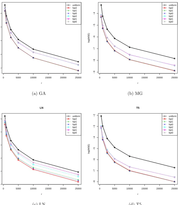
Log of the MSEs of subsampling estimator against different subsample
sizes r in Poisson regression based on the full sample estimator ˆ
β
with
n
= 50
,
000,
p
= 50.
. . . .
24
4.4
Log of the MSEs of subsampling estimator against different subsample
sizes r in Negative Binomial regression based on the full sample estimator
ˆ
β
with
n
= 50
,
000,
p
= 50.
. . . .
25
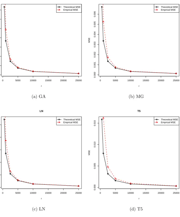
4.5
Theoretical and Empirical MSEs under ˆ
π
(2)
subsampling for Poisson
re-gression based on the full sample estimator ˆ
β
with
n
= 50
,
000,
p
= 50.
. .
27
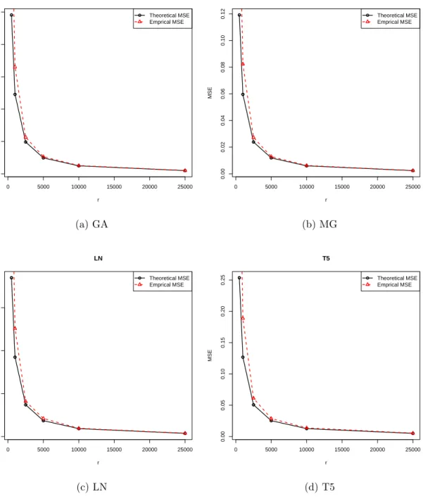
4.6
Theoretical and Empirical MSEs under ˆ
π
(2)
for Negative Binomial
regres-sion based on the full sample estimator ˆ
β
with
n
= 50
,
000,
p
= 50.
. . . .
28
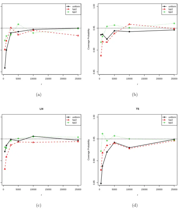
4.7
Simulated percentages of the 95% confidence intervals which caught the
true parameter
β
2
for different subsample sizes
r
, pre-subsample size
r
0
=
500 with
n
= 50
,
000,
p
= 50 under ˆ
π
(2)
, ¯
π
(2)
and uniform subsampling in
Poisson regression
. . . .
30
4.8
Simulated percentages of the 95% confidence intervals which caught the
true parameter
β
2
for different subsample sizes
r
, pre-subsample size
r
0
=
500 with
n
= 50
,
000,
p
= 50 under ˆ
π
(2)
, ¯
π
(2)
and uniform subsampling in
Negative Binomial regression
. . . .
31
5.1
Standarded deviance residuals in Quasipoisson regression model with the
casual bike rental, the registered bike rental, and the combined bike rental
as response variable.
. . . .
53
5.2
Standarded deviance residuals for Negative Binomial regression model
with the casual bike rental, the registered bike rental, and the combined
bike rental as response variable.
. . . .
54
Figure
Page
6.1
Simulated percentages of the 95% confidence intervals which caught the
full sample MLE ˆ
β
2
in Quasipoisson regression model with the casual bike
rental as the response variable, the pre-subsample size
r
0
= 200.
. . . .
63
6.2
MSE plots in Quasipoisson regression model with the casual bike rental
as the response variable, the pre-subsample size
r
0
= 200.
. . . .
64
6.3
Averages of the sum of squared predicted errors and the first several
av-erages of the sum of squared predicted errors plot in Quasipoisson
re-gression model with the casual bike rental as the response variable, the
pre-subsample size
r
0
= 200.
. . . .
66
6.4
Simulated percentages of the 95% confidence intervals which caught the
full sample MLE plot of ˆ
β
2
in Negative Binomial regression model with the
casual bike rental as the response variable, the pre-subsample size
r
0
= 200. 71
6.5
MSE plots in Negative Binomial regression model with the casual bike
rental as the response variable, the pre-subsample size
r
0
= 200.
. . . .
72
6.6
Averages of the sum of squared predicted errors and the first several
av-erages of the sum of squared predicted errors plot in Negative Binomial
regression model with the casual bike rental as the response variable, the
pre-subsample size
r
0
= 200.
. . . .
74
6.7
Simulated percentages of the 95% confidence intervals which caught the
full sample MLE plot of ˆ
β
2
in Quasipoisson regression model with the
registered bike rental as the response variable, the pre-subsample size
r
0
=
200.
. . . .
78
6.8
MSE plots in Quasipoisson regression model with the registered bike rental
as the response variable, the pre-subsample size
r
0
= 200.
. . . .
79
6.9
Averages of the sum of squared predicted errors and the first several
av-erages of the sum of squared predicted errors plot in Quasipoisson
regres-sion model with the registered bike rental as the response variable, the
pre-subsample size
r
0
= 200.
. . . .
81
6.10 Simulated percentages of the 95% confidence intervals which caught the
full sample MLE plot of ˆ
β
2
in Negative Binomial regression model with
the registered bike rental as the response variable, the pre-subsample size
r
0
= 200.
. . . .
85
6.11 MSE plots in Negative Binomial regression model with the registered bike
Figure
Page
6.12 Averages of the sum of squared predicted errors and the first several
av-erages of the sum of squared predicted errors plot in Negative Binomial
regression model with the registered bike rental as the response variable,
the pre-subsample size
r
0
= 200.
. . . .
88
6.13 Simulated percentages of the 95% confidence intervals which caught the
full sample MLE ˆ
β
2
plot in Quasipoisson regression model with the
com-bined bike rental as the response variable, the pre-subsample size
r
0
= 200. 92
6.14 MSE plots in Quasipoisson regression model with the combined bike rental
as the response variable, the pre-subsample size
r
0
= 200.
. . . .
93
6.15 Averages of the sum of squared predicted errors and the first several
av-erages of the sum of squared predicted errors plot in Quasipoisson
regres-sion model with the combined bike rental as the response variable, the
pre-subsample size
r
0
= 200.
. . . .
95
6.16 Simulated percentages of the 95% confidence intervals which caught the
full sample MLE ˆ
β
2
plot in Negative Binomial regression model with the
combined bike rental as the response variable, the pre-subsample size
r
0
= 200.99
6.17 MSE plots in Negative Binomial regression model with the combined bike
rental as the response variable, the pre-subsample size
r
0
= 200.
. . . . .
100
6.18 Averages of the sum of squared predicted errors and the first several
av-erages of the sum of squared predicted errors plot in Negative Binomial
regression model with the combined bike rental as the response variable,
the pre-subsample size
r
0
= 200.
. . . .
102
7.1
Averaged predicted sum of error squares plot in zero-inflated Poisson
ABSTRACT
Zhao, Xiaofeng Ph.D., Purdue University, August 2018. Regression Analysis of Big
Count Data Via A-Optimal Subsampling. Major Professors: Fei Tan and Hanxiang
Peng.
There are two computational bottlenecks for Big Data analysis: (1) the data is too
large for a desktop to store, and (2) the computing task takes too long waiting time
to finish. While the Divide-and-Conquer approach easily breaks the first bottleneck,
the Subsampling approach simultaneously beat both of them. The uniform sampling
and the nonuniform sampling–the Leverage Scores sampling– are frequently used in
the recent development of fast randomized algorithms. However, both approaches,
as Peng and Tan (2018) have demonstrated, are not effective in extracting
impor-tant information from data. In this thesis, we conduct regression analysis for big
count data via A-optimal subsampling. We derive A-optimal sampling distributions
by minimizing the trace of certain dispersion matrices in general estimating
equa-tions (GEE). We point out that the A-optimal distribuequa-tions have the same running
times as the full data M-estimator. To fast compute the distributions, we propose
the A-optimal Scoring Algorithm, which is implementable by parallel computing and
sequentially updatable for stream data, and has faster running time than that of the
full data M-estimator. We present asymptotic normality for the estimates in GEE’s
and in generalized count regression. A data truncation method is introduced. We
conduct extensive simulations to evaluate the numerical performance of the proposed
sampling distributions. We apply the proposed A-optimal subsampling method to
analyze two real count data sets, the Bike Sharing data and the Blog Feedback data.
Our results in both simulations and real data sets indicated that the A-optimal
distri-butions substantially outperformed the uniform distribution, and have faster running
times than the full data M-estimators.
1. INTRODUCTION
This dissertation is concerned with fast regression methods for big count data with
nonnegative integer response. Our approach is
optimal subsampling
.
1.1
Review of Regression Analysis of Count Data
Count data are observations of the number of occurrences of a behavior in a fixed
period of time. Count data are common, for example, hospital visits, blog comments,
car/bike renters, and questionnaire respondents.
Analysis of count data is an important task in social sciences and economics. Since
linear regression does not take into account the restricted number of count response
values it is not an appropriate technique for count data. Standard regression methods
include Poisson, overdispersed Poisson, negative binomial, and zero-inflated Poisson
regressions, as well as truncated methods and quasi-likelihood approach.
The Poisson regression and Negative binomial approach are often used in count
data analysis. It is motivated by the usual consideration for regression analysis,
mean-while, seek to protect and exploit the nonnegative and integer-valued characteristic
of the outcome as much as possible. The scope of count data is very wide, including
sociology, marketing, demographic economics, crime victimology, political science,
doctor visits, credit reports, recreational trips, bank failures, accident insurance,
doc-toral publications, and manufacturing defects. Count data analysis has drawn a lot
of attention and been a influential part in statistic modeling.
The most frequently used regression approach for count variables is probably
Pois-son regression. However, PoisPois-son regression requires distributional assumptions. It
is often of limited use in real data because real count data usually exhibit
over-dispersion, an inflated number of zeros, an absence of certain counts, censoring counts,
and missing counts.
Overdisperson can be addressed by generalizing the Poisson model to, for instance,
quasi-Poisson models. Another useful approach is the negative binomial regression.
These models are related to the generalized linear models family see, e.g., Nelder and
Wedderburn 1972; McCullagh and Nelder 1989; Dobson (2002).
The above models can deal with over-dispersion rather well, but are not enough
for modeling excess zeros. To address this, researchers have developed methods for
zero-inflated data by including another model component to capture zero counts.
This is done by a mixture model that unifies a count component and a point mass at
zero, see Cameron and Trivedi (2005).
To deal with truncated data and censored counts, Hurdle models were proposed
in (Mullahy 1986). These models combine a count component that is left-truncated
with a hurdle component that is right-censored.
1.2
Big Data Analysis
Big Data are on a massive scale with regard to volume, velocity, variety, and
veracity that exceed both the capacity of the conventional software tools and operating
systems and the physical spaces of computers, see e.g. Wang,
et al.
(2015); Fan,
et
al.
(2013). Massive data pose two computational bottlenecks: (1) the data exceed
a computer’s memory, and (2) the computing task requires too long waiting time to
finish. The two bottlenecks can be simultaneously addressed by
judiciously
choosing
a sub-data as a surrogate for the full data and completing the data analysis. This is
the goal that this dissertation will pursue.
While the often used Divide-and-Conquer approach readily breaks the memory
limit, the proposed subsampling approach not only breaks the limit but speed up
computing as well as possesses other useful statistical properties. Due to its
math-ematical simplicity and computational ease, the
uniform sampling
is often used in
subsampling for intensive computing and for development of fast randomized
algo-rithms and in re-sampling for Monte Carlo and bootstrap. The uniform sampling,
however, is not effective in extracting information, see a simulation study in in Peng an
Tan (2018). In this dissertation, non-uniform sampling distributions on data points
by the criterion of A-optimality will be sought, that is, by minimizing the trace
of certain variance-covariance matrix. Equivalently, Distributions will be sought to
minimizing the sum of the component variances of certain subsampling estimate.
Mathematicians, computer scientists and statisticians have already made important
progress in this area. Drineas,
et al.
(2006a) constructed fast Monte Carlo algorithms
to approximate matrix multiplication. Drineas,
et al.
(2006b) presented a sampling
algorithm for the least squares fit problem and studied its algorithmic properties.
A key feature of the above algorithms is the non-uniform sampling. Ma and Sun
(2014) and Ma,
et al.
(2015) used the leverage scores as non-uniform importance
sampling distributions for big data linear regression. Zhu,
et al.
(2015) obtained
opti-mal subsampling distributions for large sample linear regression. Wang,
et al.
(2015)
constructed optimal subsampling for large logistic regression. Xu,
et al.
(2016)
stud-ied subsampled newton methods with non-uniform sampling. Wang,
et al.
(2017)
developed information-based subdata selection for large linear regression. Peng and
Tan (2018a, 2018b) investigated A-optimal subsampling for Big Data linear regression
and constructed fast algorithms. Liang,
et al.
(2013) proposed a resampling-based
stochastic approximation for large geostatistical data. Kleiner,
et al.
(2014) gave a
scalable bootstrap for massive data. Avron,
et al.
(2010) used random-sampling and
random-mixing techniques to describe a fast LS solver for dense highly
overdeter-mined systems. Drineas,
et al.
(2010) constructed randomized algorithms for faster
least squares approximation. See also the monograph by Mahoney (2011) on
nonuni-form random subsampling for matrix based machine learning.
Fan
et al.
(2014) proposed salient features of big data such as heterogeneity, noise
accumulation, spurious correlation and incidental endogeneity. Two very commonly
used method to handle big data issue are Divided and Conquer and the Subsampling.
The uniform subsmapling is simple in mathematics and easy in computation, so it
is frequently used, such as Monte Carlo and bootstap method. Unfortunately, the
uniform sampling can not detect important observations. Ma,
et al.
(2014) conduct
the leverage score based non-uniform subsampling method, this method used the
esti-mate from a subsample taken randomly from the full sample to approxiesti-mate the full
sample ordinary least square estimate, they proposed BLEV,SLEV,and LEVUNW
method to perform subsampling. Drineas,
et al.
(2004) proposed the non-uniform
distribution to develop fast algorithms to approximate the product of two matrices,
the idea is to minimize the expected squared Frobenius distance of the product and
its approximate. Ma
et al.
(2015) proposed the OPT and PL subsampling method in
linear regression model, they discussed the sampling probability by minimizing the
trace of the intermittent part of the variance-covariance matrix of the subsampling
estimator, derived asymptotic normality and performed simulations and real data
analysis. Peng and Tan (2018) derived asymptotic expansions for the subsampling
estimator and the asymptotic normality under appropriate conditions in linear
re-gression model, proposed A-optimal probability distribution to estimate a smooth
function of the regression coefficient, proposed data truncation for fast computing.
Wang,
et al.
(2017) proposed non-uniform subsampling probabilities that minimize
the asymptotic mean squared error of subsampling estimator in logistic regression,
established consistency and asymptotic normality of the estimator.
This dissertation will develop the A-optimal subsampling theory for arbitrary
data structure and general estimating procedures. These results are parallel to those
obtained in the linear regression model in Peng and Tan (2018a).
Since we are
concerned with a resampling procedure, the data structure can be
arbitrary
. That
is, data can be random or deterministic, dependent or independent, complete or
incomplete (missing/censored/truncated), time-series data, longitudinal data, spatial
correlated data, etc. We shall pursue both the algorithmic properties (i.e. how long
it takes to compute the approximating subsampling estimator), and the statistical
inference (i.e. under what conditions the approximating subsampling estimator is
valid). We shall focus on fast algorithms, parallel computing, sequential updating and
subsample size determination for the former, and on deriving A-optimal distributions,
asymptotic normality, and dimension asymptotics (how growing dimensions affect the
subsampling estimates) for the latter.
The rest of the thesis is organized as follows. In Chapter 2, we introduce the
Count data regression and demonstrate several examples. In Chapter 3, we study the
A-optimal subsampling distributions and establish the consistency and asymptotic
normality theorem. We report the large simulation results in Chapter 4. In chapter
5, 6, we report the real count data analysis of the Bike Sharing data. In chapter 7,
we report the real count data analysis of the Blog Feedback data.
2. COUNT DATA REGRESSION
In a count data regression model, the mean of a count response
Y
i
and covariate
vector
x
i
satisfy
E
(
Y
i
) =
µ
i
(
β
) =
h
(
x
>
i
β
)
,
i
= 1
, . . . , n,
(2.0.1)
where
β
∈
R
p
is a regression parameter and
h
is an inverse link function. Typically,
h
(
t
) = exp(
t
) (the inverse log link).
2.1
Poisson Regression, Overdisperson and Negative Binomial
Regres-sion
The Poisson distribution is commonly used for modeling count data.
Example 1
Let
Y
has Poisson distribution with mean parameter
µ
, Poi(
µ
). Then
the probability mass function of
Y
is given by
f
poi
(
y
;
µ
) = exp(
−
µ
)
µ
y
y
!
,
y
= 0
,
1
,
2
, . . .
(2.1.1)
For a Poisson random variable
Y
, the mean and variance are equal, Var(
Y
) =
µ
=
E
(
Y
). In real data, the equality of mean and variance is usually not met. This is
termed as
overdisperson
.
When overdispersion occurs in a real data, the SE of estimates in Poisson
regres-sion model are deflated, leading to exaggerated test statistic for parameters and hence
false significant findings. Overdispersion can often be tested by the usual goodness
of fit statistic. In our real data analysis, we should perform such tests.
Example 2
Let
Y
have a negative binomial distribution with mean
µ
and
overdis-person parameter
α >
0, Nb(
µ, α
). Then the probability mass function of
y
is given
by
f
nb
(
y
;
µ, α
) =
Γ(
y
+ 1
/α
)
Γ(1
/α
)
y
!
(1 +
αµ
)
−
1
/α
(
µ/
(
µ
+ 1
/α
))
−
y
, y
= 0
,
1
,
2
, . . .
(2.1.2)
For a negative binomial random variable
Y
, the mean
E
(
Y
) =
µ
and variance
Var(
Y
) =
µ
+
αµ
2
satisfy Var(
Y
)
≥
E
(
Y
), and Var(
Y
) =
E
(
Y
) if and only if
α
= 0.
Another powerful option to handle overdisperson is the
quasi-likelihood model
.
This has the advantage of requiring only to specify the mean and variance but not a
distribution for the response
Y
. Specifically, the statistical inference is based on the
quasi-likelihood equation,
n
X
i
=1
y
i
−
µ
i(
β
)
V
i
(
β, φ
)
h
0
(
x
>
i
β
)
x
i
= 0
,
(2.1.3)
where
µ
i
(
β
) =
E
(
Y
i
|
x
i
) and
V
i
(
β, φ
) = Var(
Y
i
|
x
i
) are the mean function and variance
function which are to be specified. Here
φ
is an overdisperson parameter.
The quasi-likelihood model has great flexibility and unifies several models in the
sense that the maximum likelihood estimate (MLE) of the models are special cases.
Setting
V
i
=
µ
i
, equation (2.1.3) gives the MLE of the Poisson model.
If
V
i
=
µ
i
(1 +
αµ
i
) with
φ
=
α
, then equation (2.1.3) is the estimating equation for the
MLE of the negative binomial model. Another frequent choice of the variance for
overdisperson is
V
i
=
φµ
i
with
φ >
0.
All the three cases can be unified with
V
i
=
µ
i
+
αµ
p
i
for
p
= 1
,
2.
2.2
Zero-inflated Poisson Regression
In many real count data, there is an excess of zero counts for which the Poisson
distribution can not account. Consider a mixture model combining a degenerate
distribution at 0 and a Poisson distribution defined by
where
f
0
(
y
) =
1
[
y
= 0] is the point mass at zero (the degenerate distribution at zereo)
to account for structural zeros. Since
f
zip
(0;
µ, ρ
) =
ρ
+ (1
−
ρ
) exp(
−
µ
)
,
it thus follows from 0
≤
f
zip
(0;
µ, ρ
)
≤
1 that 1
/
(1
−
exp(
µ
))
≤
ρ
≤
1. This shows
that
ρ
can be negative. A positive
ρ
represents the probability of structural zeros
above the amount of zeros expected under the Poisson distribution
f
poi
. A negative
ρ
means that the amount of zeros is below the expected under Poisson, and this does
not occur very often. The MLE ˆ
β
n
can be obtained by solving the score equation
n
X
i
=1
f
poi
(
y
i;
µ
i)
f
zip
(
y
i
;
µ
i
, ρ
)
y
i
−
µ
i(
β
)
µ
i
(
β
)
h
0
(
x
>
i
β
)
x
i
= 0
.
(2.2.2)
To estimate
ρ
, one can obtain another equation differentiating the log likelihood
with respect to
ρ
. For simplicity, we shall estimate
ρ
by the sample percentage ˆ
ρ
of
structural zeros. Substituting ˆ
ρ
in (2.2.2), we solve for ˆ
β
n
.
2.3
Truncated Models
Suppose realizations of a count random variable
Y
less than a positive integer
l
are
omitted. Then the resulting distribution is called
left-truncated
. For simplicity, only
left-truncation is considered and right-truncation is similar. Let
Y
has pmf
g
(
y
;
θ
)
and cdf
G
(
y
;
θ
) with parameter
θ
. Then left-truncated count distribution is given by
f
(
y
;
θ
|
y
≥
l
) =
¯
g
(
y
;
θ
)
G
(
l
−
1;
θ
)
,
y
=
l, l
+ 1
, . . . ,
(2.3.1)
where ¯
G
= 1
−
G
is the survival function.
Choosing
g
to be the pmf of the negative binomial, the left-truncated negative
binomial can be obtained. As a limiting case of this, the left truncated distribution
of Poisson Poi(
µ
) can be obtained as follows:
f
(
y
;
µ
|
y
≥
l
) =
µ
y
(exp(
µ
)
−
P
l
−
1
i
=1
µ
i
/i
!)
y
!
This has the mean
E
(
Y
) =
µ
+
δ
and variance Var(
Y
) =
µ
−
δ
(
µ
−
l
), where
δ
=
f
¯
poi
(
l
−
1;
µ
)
F
poi
(
l
−
1;
µ
)
µ.
(2.3.3)
These exhibit that the mean of the left-truncated random variable is bigger than the
corresponding mean of the un-truncated distribution, whereas the truncated variance
is smaller. The MLE of ˆ
β
n
can be obtained as the solution of the following equation
n
X
i
=1
y
i
−
µ
i
(
β
)
−
δ
i
(
β
)
µ
i
(
β
)
h
0
(
x
>
i
β
)
x
i
= 0
.
(2.3.4)
2.4
Censored Counts
Censoring of count observations may arise from aggregation or from the resulting
samples in which high counts are not observed. Health data and social media data
are examples. Consider a latent count variable
Z
that is censored from above at point
c
(right censoring) and covariate variable
x
. Let
Y
=
Z
if
Z
≤
c
. Suppose
Z
satisfies
the regression model
Z
=
µ
(
x
;
β
) +
ε,
(2.4.1)
where
ε
is a random error with mean
E
(
ε
) = 0. Suppose there are available
inde-pendent observations (
Y
i
, d
i
,
x
i
)
, i
= 1
, . . . , n
, where
d
i
=
1
[
Z
i
≤
c
] is the censoring
indicator, and
Y
i
=
Z
i
if
δ
i
= 1. Suppose
Y
has pmf
g
(
y
;
θ
) and cdf
G
(
y
;
θ
). The
log-likelihood function for the independent observations are
`
n
(
β
) =
n
X
i
=1
d
i
log
g
(
Y
i
;
θ
(
β
)) + (1
−
d
i
) log ¯
G
(
c
−
1;
θ
(
β
))
.
(2.4.2)
For the right censored Poisson model, the maximum likelihood estimating equation
is given by
n
X
i
=1
d
i
(
Y
i
−
µ
i
(
β
)) + (1
−
d
i
)
δ
i
(
β
)
µ
i
(
β
)
h
0
(
x
>
i
β
)
x
i
= 0
.
(2.4.3)
where
δ
i
(
β
) is the adjustment factor associated with the left-truncated Poisson model,
given by
δ
i
(
β
) =
f
poi
(
c
−
1;
µ
i
(
β
))
¯
F
poi
(
c
−
1;
µ
i
(
β
))
µ
i
(
β
)
.
(2.4.4)
3. A-OPTIMAL SAMPLING DISTRIBUTIONS AND
ASYMPTOTIC THEORY
Let
{
Z
ni
: 1
≤
i
≤
n, n
≥
1
}
be a sequence of random variables defined on some
probability space (Ω
,
P
) and
β
∈ B ⊂
R
p
be a parameter vector. Consider a triangular
array of smooth functions
{
ψ
ni
(
Z
ni
;
β
): 1
≤
i
≤
n
,
n
≥
1
}
taking values in
R
p
with
each
E
(
ψ
ni
(
Z
ni
;
β
0
)) = 0 for a unique
β
0
∈ B
. We estimate
β
0
by ˆ
β
n
which solves the
estimating equations,
Ψ
n
(
β
) =
n
X
i
=1
ψ
ni
(
Z
ni
;
β
) = 0
.
(3.0.1)
Following Chatterjee and Bose (2005), we assume
{
(
ψ
ni
(
Z
ni
;
β
0
)
,
F
i
)
, i
= 1
, . . . , n, n
≥
1
}
forms a martingale difference, i.e.,
E
(
ψ
ni(
Z
ni;
β
0
)
|
F
i
−
1
) = 0, where
{
F
i
, i
=
1
,
2
, . . . ,
}
is an increasing sequence of sigma-algebras, see Chapter 5 of Borovskikh
and Korolyuk (1974).
We consider the case that the sample size
n
is
extremely large
and the estimate
ˆ
β
n
is not available or time-consuming to obtain it. Our approach to tackling this big
data estimation problem is
A-optimal subsampling
, that is, we seek the A-optimal
sampling distribution on the data points and use it take a subsample as a surrogate
of the whole sample.
Let
π
n
= (
π
ni
, i
= 1
, . . . , n
) be a sampling distribution on the
n
data points
Z
ni
. We use it to take a subsample
Z
∗
=
{
Z
j
∗
:
j
= 1
, . . . , r
}
with the subsample size
r << n
. Let
π
∗
= (
π
j
∗
:
j
= 1
, . . . , r
) be the corresponding sampling probabilities. We
now approximate the estimate ˆ
β
n
by the subsampling generalized bootstrap estimate
ˆ
β
r
∗
nwhich solves the estimating equations
Ψ
∗
r
(
β
) =:
r
X
j
=1
ψ
nj(
Z
nj
∗
;
β
)
π
∗
j
= 0
.
(3.0.2)
The theory of weighted (generalized) bootstrap has been extensively studied in the
literature, see e.g. Mammen (1993) and Chatterjee and Bose (2002). However, the
choices in existing weights are limited; most of them are exchangeable non-negative
random variables that are independent of data; and only some of them can improve
Efron’s bootstrap using tedious Edgeworth expansions. See Chapter II of the
mono-graph by Barbe and Bertail (1995) and the references therein. Unlike existing weights,
we shall allow the weights to depend on the data. In fact, we shall derive numerous
weights by minimizing the trace of certain variance-covariance. They are referred to
as the A-optimal weights which are different from existing weights: they are data
driven so dependent of the data and not exchangeable.
3.1
A Theorem from Chung, Tan and Peng (2018)
Notation
. Abbreviate
ψ
ni
(
β
) =
ψ
ni
(
Z
ni
;
β
), its
d
-th component
ψ
ni,d
(
β
), and
ψ
ni
=
ψ
ni
(
β
0
). Let ˙
ψ
ni
(
β
) =
∂/∂βψ
ni
(
β
)
∈
R
p
and ¨
ψ
ni
(
β
) =
∂/∂β
>
ψ
˙
ni
(
β
) (
p
×
p
matrix) be the first and second partial derivatives with respect to parameter
β
. For
matrix
A
, denote
A
>
the transpose of
A
,
A
⊗
2
=
AA
>
,
A
−>
= (
A
−
1
)
>
,
E
−
1
(
A
) =
(
E
(
A
))
−
1
, and
A
(
s
)
= 1
/
2(
A
+
A
>
). Write
k
A
k
the euclidean norm,
k
A
k
o
the spectral
norm,
λ
max
(
A
) (
λ
amin
(
A
)) the maximum (minimum absolute) eigenvalue of
A
, etc.
To quote a theorem from Chung, Tan and Peng (2018), we introduce the following
assumptions. Let
J
n
(
β
) =
n
X
i
=1
π
−
ni
1
ψ
ni
(
β
)
⊗
2
, λ
n
=
λ
1
max
/
2
(
J
n
( ˆ
β
n
))
,
Σ
n
= ˙
Ψ
−
n
1
J
n
Ψ
˙
−>
n
ˆ
β
n.
(3.1.1)
Let
δ
n
>
0 be an arbitrary sequence. Typically,
δ
n
= min(
π
ni
, i
= 1
, . . . , n
).
(R1)
δ
n
λ
2
n
p
−→ ∞
,
P
(
δ
−
1
n
λ
−
2
n
λ
amin
( ˙
Ψ
(
s
)
n
( ˆ
β
n
))
>
0)
→
1
.
(R2) Each component
ψ
ni,d
(
β
) admits the second order expansion
ψ
ni,d
(
β
0
+
t
) =
ψ
ni,d
(
β
0
) + ˙
ψ
ni,d
>
(
β
0
)
t
+ 1
/
2
t
>
ψ
¨
ni,d
( ˜
β
ni,d
)
t,
d
= 1
, . . . , p,
(R3) The sampling probabilities
π
ni
and subsample size
r
n
satisfy
n
X
i
=1
π
−
ni
1
k
ψ
˙
ni
( ˆ
β
n
)
k
2
=
o
p
(
p
−
n
1
r
n
δ
n
2
λ
4
n
)
.
(R4) There exists a neighborhood
N
0
of
β
0
such that ¨
Ψ
n,d
(
β
) is either positive or
negative definite in
N
0
and that there is a rv
η
ni,d
sup
β
∈
N0
λ
amax
( ¨
Ψ
n,d
(
β
))
≤
η
ni,d
,
d
= 1
, . . . , p,
where the random vector
η
ni
= (
η
ni,
1
, . . . , η
ni,p
)
>
satisfies
n
X
i
=1
(
n
+ (
r
n
π
ni
)
−
1
)
k
η
ni
k
2
=
o
p
(
p
−
n
2
r
n
δ
n
4
λ
6
n
)
.
(R5)
λ
max
(
J
n
( ˆ
β
n
))
/λ
min
(
J
n
( ˆ
β
n
)) =
O
p
(1)
.
(R6) Fix
u
∈
R
p
nwith
k
u
k
= 1. The double array
z
∗
nj
=
s
−
1
n
u
>
Ψ
˙
−>
n
( ˆ
β
n
)
ψ
∗
nj
( ˆ
β
n
)
/π
∗
nj
,
j
= 1
,
2
, . . . , r, r
≥
1 satisfies the Lindeberg condition: for every
t >
0,
n
X
i
=1
π
ni
k
z
n,i
k
2
1
[
k
z
ni
k ≥
√
rt
] =
o
p
(1)
,
as
r
→ ∞
,
where
s
2
n
=
u
>
Σ
n
u
.
We quote the following theorem from Chung, Tan and Peng (2018).
Theorem 3.1.1
Suppose (R1)–(R5) hold. Assume
β
ˆ
n
is a solution of (3.0.1) such
that
β
ˆ
n
=
β
0
+
o
p
(1)
. Assume
n
X
i
=1
π
−
ni
1
k
ψ
ni
( ˆ
β
n
)
k
2
=
O
p
(
p
n
λ
2
n
)
.
(3.1.2)
Then these exists a sequence of solutions
β
ˆ
r
∗
nof (3.0.2) such that if
p
n
/
(
r
n
δ
n
2
λ
2
n
) =
o
p
(1)
, then
˙
Ψ
n
( ˆ
β
n
)
√
r
n
( ˆ
β
r
∗
n−
ˆ
β
n
) =
−
1
√
r
n
r
nX
j
=1
ψ
nj
∗
( ˆ
β
n
)
π
∗
j
+
o
p
(
λ
n
)
.
(3.1.3)
If, further, (R5)–(R6) are satisfied for
u
∈
R
r
nwith
k
u
k
= 1
, then
s
−
n
1
√
r
n
u
>
( ˆ
β
∗
r
n−
ˆ
3.2
A Second Theorem from Chung, Tan and Peng (2018)
Let
J
1
n
(
β
) =
n
X
i
=1
E
(
ψ
ni
(
β
)
⊗
2
)
,
λ
1
n
=
λ
1
max
/
2
(
J
1
n
)
.
(R1’)
λ
1
n
→ ∞
,
inf
n
≥
n
0{
λ
−
2
1
n
λ
amin
(
E
( ˙
Ψ
n
(
s
)
))
}
>
0
.
(R3’)
P
n
i
=1
E
k
ψ
˙
ni
−
E
( ˙
ψ
ni
)
k
2
=
o
(
p
−
1
n
λ
4
1
n
)
.
(R4’) Same as (R4) except that
η
ni
are replaced with
η
1
ni
which satisfy
n
X
i
=1
k
η
1
ni
k
2
=
o
p
(
n
−
1
p
−
n
2
λ
6
n
)
.
(R5’)
λ
max
(
J
1
n
)
/λ
min
(
J
1
n
) =
O
(1)
.
(R6’) Fix
u
∈
R
p
nwith
k
u
k
= 1. Let
s
2
1
n
=
u
>
E
−
1
( ˙
Ψ
n
)
P
n
i
=1
ψ
⊗
2
ni
E
−>
( ˙
Ψ
n
)
u
. The
double array
z
1
ni
=
s
−
1
n
1
u
>
E
−
1
( ˙
Ψ
n
)
ψ
ni
,
i
= 1
,
2
, . . . , n, n
≥
1 satisfies
n
X
i
=1
k
z
1
ni
k
2
=
o
p(1)
,
E
(max
i
k
z
1
ni
k
) =
o
(1)
.
for every
t >
0.
We quote the following theorem from Chung, Tan ane Peng (2018), which describes
the asymptotic behaviors of the M-estimator for both fixed and growing parameter
dimension.
Theorem 3.2.1
Suppose (R1’), (R2), (R3’)–(R5’) hold. Then these exists a
se-quence of solutions
β
ˆ
n
of (3.0.1) such that if
p
n
/λ
2
1
n
=
o
(1)
, then
p
−
n
1
/
2
λ
1
n
( ˆ
β
n
−
β
0
) =
O
p
(1)
,
(3.2.1)
λ
−
1
n
1
E
( ˙
Ψ
n
)( ˆ
β
n
−
β
0
) =
−
λ
−
1
n
1
n
X
i
=1
ψ
ni
+
o
p
(1)
.
(3.2.2)
If, further, (R5’)–(R6’) are satisfied for
u
∈
R
p
with
k
u
k
= 1
, then
3.3
The A-optimal Sampling Distribution
In view of Theorem 3.1.1 and (3.1.1), we have
Var
∗
( ˆ
β
r
∗
n) =
1
r
Σ
n
+
o
p
(1) =
1
r
n
X
i
=1
1
π
i
˙
Ψ
−
n
1
ψ
ni
ψ
>
ni
Ψ
˙
−>
n
|
β
ˆ
n+
o
p
(1)
.
(3.3.1)
As Σ
n
is a function of the sampling distribution
π
= (
π
1
, . . . , π
n
) on the data points,
we seek a sampling distribution which minimizes the trace of the matrix Σ
n
. Following
Peng and Tan (2018), we write
τ
(
π
) =: Tr Σn) =
n
X
i
=1
k
a
ni
k
2
π
i
,
π
∈
P
n
,
where
a
ni
= ˙
Ψ
−
n
1
ψ
ni
|
β
ˆ
n, and
P
n
is the probability simplex
P
n
=
{
π
:
π
i
≥
0
,
P
i
π
i
=
1
}
in
R
n
. Using Lagrange multipliers, we readily derive the minimizer which is stated
in the following theorem. As usual, the minimizer is referred to as
A-optimal
.
Equiv-alently, an A-optimal distribution minimizes the sum of the component variances of
the subsampling estimator ˆ
β
r
∗
n
. Let
ˆ
H
k
=
A
n
( ˙
Ψ
>
n
Ψ
˙
n
)
−
k/
2
A
>
n
|
β
ˆ
n,
k
= 0
,
1
,
2
.
(3.3.2)
where
A
n
(
β
) = (
ψ
n
1
(
β
)
, . . . , ψ
nn
(
β
))
>
. The following theorem is quoted from Chung,
Tan and Peng (2018).
Theorem 3.3.1
Suppose
Ψn( ˆ
˙
β
n)
is invertible. Then the square roots of the diagonal
entries of
H
ˆ
2
gives an (asymptotically) A-optimal distribution
π
ˆ
on the data points
for
β
ˆ
r
∗
nto approximate
β