ABSTRACT
YI, TING. Travel Time Estimation from Fixed Point Detector Data. (Under the direction of Dr. Billy M. Williams).
Travel time, as a fundamental measurement for Intelligent Transportation Systems, is becoming increasingly important. Due to the wide deployment of the fixed point detectors on freeways, if travel time can be accurately estimated from point detector data, the indirect estimation method is cost-effective and widely applicable. This dissertation presents a systematic method for accurately estimating the travel time of different freeway links under various traffic conditions using fixed-point detector data.
Travel Time Estimation from Fixed Point Detector Data
by Ting Yi
A dissertation submitted to the Graduate Faculty of North Carolina State University
in partial fulfillment of the requirements for the degree of
Doctor of Philosophy
Civil Engineering
Raleigh, North Carolina 2009
APPROVED BY:
_______________________________ ______________________________ Dr. Billy M. Williams Dr. Nagui M. Rouphail
Committee Chair
DEDICATION
BIOGRAPHY
ACKNOWLEDGEMENTS
I would like to express my sincerest gratitude to my advisor, Dr. Billy Williams, for his guidance, patience, understanding and kindness during my graduate study at North Carolina State University. I want to thank him for sharing his wisdom and helping me out whenever I was at loss on my research. It was personally a rewarding experience to work with Dr. Williams.
I would like to thank Dr. Nagui Rouphail, Dr. Joseph Hummer and Dr. Peter Bloomfield for serving on my advisory committee and providing their invaluable expertise to achieve my goals. I want to thank Dr. Rouphail for giving me the opportunity to study at NCSU, and for his excellent teaching. I am also indebted to Dr. Williams, Dr. Bloomfield and Dr. John Stone for the knowledge through the courses. Special thanks to Dr. Hummer for his help and support when I work for him.
Special thanks to Dr. Qianyi Zhang, Mr. Qiang Jin, Dr. Jae-Pil Moon and Mrs. Wen Huang for the technique help. I also want to thank Dr. Yongping Zhang, Mr. Slade McCalip, Dr. Yang Han and Dr. Xiaojin Ji for the help and guidance during my industry work. And thanks to Ting, Rong, Miao, Zheng, Shanshan, Hongqiong, Lu, Isaac, Alex, Jisun for the good times.
Generation Simulation (NGSIM) Program data provided to accomplish the dissertation.
TABLE OF CONTENTS
LIST OF TABLES --- x
LIST OF FIGURES --- xii
CHAPTER I INTRODUCTION --- 1
1.1BACKGROUND --- 1
1.2MOTIVATION --- 2
1.3PROBLEM STATEMENT --- 3
1.3.1 Section Travel Time Definition --- 3
1.3.2 Problem Definition of Travel Time Estimation from Fixed Point Detector Data --- 5
1.3.3 Ideal Travel Time Estimation Methods --- 11
1.4OBJECTIVE AND SCOPE --- 12
1.5RESEARCH METHODOLOGY --- 14
1.6DISSERTATION ORGANIZATION --- 16
CHAPTER 2 LITERATURE REVIEW --- 18
2.1CLASSIFICATION OF METHODS FOR OBTAINING TRAVEL TIME DATA --- 18
2.1.1 Direct Measurement Methods --- 18
2.1.2 Indirect Estimation Methods --- 21
2.2METHODOLOGICAL HIGHLIGHTS OF TRAVEL TIME COLLECTION METHODS --- 24
2.2.1 Traditional Floating Car Method --- 24
2.2.3 Global Positioning System (GPS) --- 27
2.2.4 License Plate Matching --- 29
2.2.5 Cellular Phone Tracking --- 31
2.2.6 Automatic Vehicle Identification (AVI) --- 32
2.2.7 Automatic Vehicle Location (AVL) --- 33
2.2.8 Speed Extrapolation --- 35
2.2.9 Probabilistic Regression --- 37
2.2.10 Cross-Correlation --- 39
2.2.11 Dynamic Traffic Flow Approach --- 41
2.2.12 Vehicle Signature Matching --- 43
2.3SUMMARY --- 44
CHAPTER 3 TRAVEL TIME ESTIMATION MODELS AND SIMULATION STUDY --- 48
3.1DESCRIPTION AND MODIFICATION OF THE THREE TRAVEL TIME ESTIMATION MODELS --- 48
3.1.1 Speed Extrapolation Models --- 49
3.1.2 Flow-based Statistic Models --- 64
3.1.3 Dynamic Traffic Flow Models --- 79
3.1.4 Summary --- 97
3.2 SIMULATION STUDY --- 98
3.2.1 Simulation Design --- 99
3.2.3 Travel Time Estimation Obtained from the Models --- 106
3.2.4 Traffic Conditions Determination --- 109
3.2.5 Comparison of the Estimated Results --- 112
3.2.6 Conclusions --- 119
3.3SUMMARY --- 121
CHAPTER 4 SYSTEMATIC METHOD --- 122
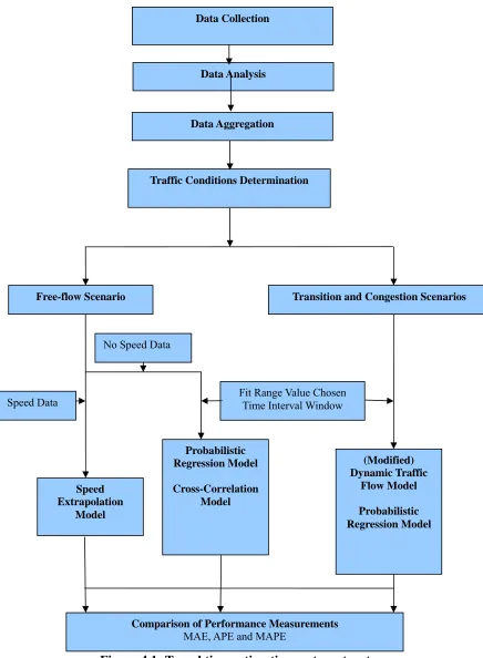
4.1PROPOSED SYSTEMATIC METHOD FRAMEWORK --- 122
4.2TRAFFIC DATA INVESTIGATION AND ANALYSIS --- 124
4.3TRAFFIC CONDITION DETERMINATION --- 128
4.4SPECIFIC MODEL SELECTION FOR TRAVEL TIME ESTIMATION--- 130
4.5PERFORMANCE MEASUREMENTS --- 141
4.6PRELIMINARY FINDINGS OF SIMULATION STUDY USING THE SYSTEMATIC METHOD 141 4.7SUMMARY --- 149
CHAPTER 5 FIELD DATA STUDY --- 150
5.1FIELD DATA DESCRIPTION --- 150
5.1.1 NGSIM US 101 Data --- 151
5.1.2 NGSIM Prototype I-80 Data --- 153
5.1.3 New I-80 Data --- 154
5.2FIELD DATA ANALYSIS AND TRAFFIC CONDITION DETERMINATION --- 156
5.2.1 Time Interval Length Identification --- 157
5.2.2 Testing of Frequency Changes in the Traffic Parameters --- 158
5.3TRAVEL TIME ESTIMATION AND PERFORMANCE MEASUREMENT --- 161
5.4CONCLUSIONS --- 170
5.5SUMMARY --- 174
CHAPTER 6 CONCLUSIONS --- 175
6.1SUMMARY --- 175
6.2MAJOR FINDINGS AND CONTRIBUTIONS --- 177
6.3FUTURE RESEARCH --- 180
REFERENCES --- 182
APPENDIX A TRAVEL TIME ESTIMATION AND PERFORMANCE MEASURE IN CHAPTER 3 --- 189
APPENDIX B MEASUREMENT RESUTES FROM SIMULATION DATA USING SYSTEMATIC METHOD IN CHAPTER 4 --- 235
APPENDIX C --- 248
LIST OF TABLES
Table 2.1 Overview of the Travel Time Methods --- 46
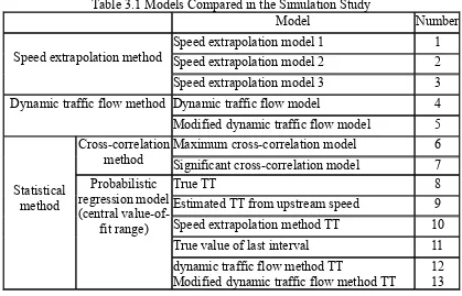
Table 3.1 Models Compared in the Simulation Study --- 98
Table 3.2 Raw Data and True Value in the Simulation Study --- 105
Table 3.3 Raw Data Aggregation in the Simulation Study --- 105
Table 3.4 Travel Time Estimates by Speed Extrapolation Models --- 106
Table 3.5 Travel Time Estimates by (Modified) Dynamic Traffic Flow Model --- 107
Table 3.6 Travel Time Estimates by Proposed Modified Dynamic Traffic Flow Model --- 107
Table 3.7 Travel Time Estimates by Proposed Modified Dynamic Traffic Flow Model --- 108
Table 3.8 Data Set to Illustrate the Determination of the Traffic Conditions --- 111
Table 3.9 Comparison of the Estimation Errors of 500m one-lane link --- 217
Table 3.10 Comparison of the Estimation Errors of 500m two-lane link --- 219
Table 3.11 Comparison of the Estimation Errors of 500m three-lane link --- 221
Table 3.12 Comparison of the Estimation Errors of 750m one-lane link --- 223
Table 3.13 Comparison of the Estimation Errors of 750m two-lane link --- 225
Table 3.14 Comparison of the Estimation Errors of 750m three-lane link --- 227
Table 3.15 Comparison of the Estimation Errors of 1000m one-lane link --- 229
Table 3.16 Comparison of the Estimation Errors of 1000m two-lane link --- 231
Table 4.1 Estimation Errors of 500m freeway link by Systematic Method --- 245
Table 4.2 Estimation Errors of 750m freeway link by Systematic Method --- 246
Table 4.3 Estimation Errors of 1000m freeway link by Systematic Method --- 247
Table 4.4 Error Comparison under Transition Condition --- 144
Table 4.5 Error Comparison under Congestion Condition--- 145
Table 4.6 Error Comparison of the 500-Meter Freeway Link --- 147
Table 4.7 Error Comparison of 750-Meter Freeway Link --- 148
Table 4.8 Error Comparison of 1000-Meter Freeway Link --- 148
Table 5.1 Traffic Condition Determination per time division for Field Data --- 281
Table 5.2 MAE and MAPE of Travel Time Estimation for US 101 Dataset --- 163
Table 5.3 MAE and MAPE of Travel Time Estimation for New I-80 Dataset --- 166
Table 5.4 MAE and MAPE of Travel Time Estimation for Prototype I-80 Dataset --- 169
LIST OF FIGURES
Figure 1.1 A temporal and spatial illustration of section travel time (source: Chu et al.
2005, Figure 1). --- 5
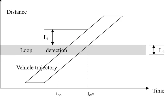
Figure 1.2 Typical freeway section with Inductive Loop Detectors. --- 6
Figure 1.3: Traffic state propagation at different time intervals. --- 9
Figure 3.1: One vehicle passing over a single-loop detector. --- 50
Figure 3.2: One vehicle passing over a dual-loop detector. --- 53
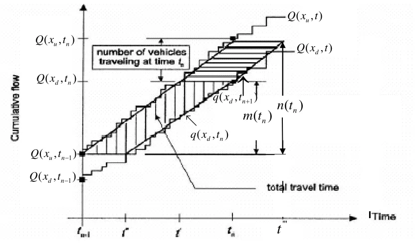
Figure 3.3: Schematic representation of the total travel time during the interval (tn-1, tn) under normal-flow conditions. (Source: Nam and Drew, 1999, Figure 2) --- 85
Figure 3.4: Schematic representation of the total travel time during the interval (tn-1, tn) under congested flow conditions. (Source: Nam and Drew, 1999, Figure 4) --- 87
Figure 3.5: Schematic representation of the total travel time during the interval (tn-1, tn) under normal-flow conditions. (Source: Vanajakshi et al., 2008, Figure 6a) --- 90
Figure 3.6: Schematic representation of the total travel time during the interval (tn-1, tn) if ( ) 0m tn > . (Source: Vanajakshi et al., 2008, Figure 6a) --- 93
Figure 3.7: Schematic representation of the total travel time during the interval (tn-1, tn) if ( ) 0m tn ≤ . (Source: Nam and Drew, 1999, Figure 4) --- 95
Figure 3.8: Car-following model parameters in the simulation design. --- 101
Figure 3.9: Lane-changing model parameters in the simulation design. --- 101
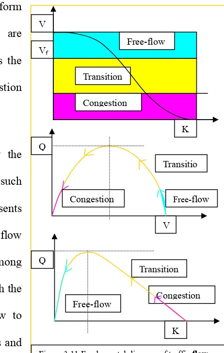
Figure 3.11 Fundamental diagram of traffic flow --- 109
Figure 3.12 Travel time estimates of 500m one-lane link at 2min interval --- 190
Figure 3.13 Travel time estimates of 500m one-lane link at 5min interval --- 191
Figure 3.14 Travel time estimates of 500m one-lane link at 10min interval --- 192
Figure 3.15 Travel time estimates of 500m two-lane link at 2min interval --- 193
Figure 3.16 Travel time estimates of 500m two-lane link at 5min interval --- 194
Figure 3.17 Travel time estimates of 500m two-lane link at 10min interval --- 195
Figure 3.18 Travel time estimates of 500m three-lane link at 2min interval --- 196
Figure 3.19 Travel time estimates of 500m three-lane link at 5min interval --- 197
Figure 3.20 Travel time estimates of 500m three-lane link at 10min interval --- 198
Figure 3.21 Travel time estimates of 750m one-lane link at 2min interval --- 199
Figure 3.22 Travel time estimates of 750m one-lane link at 5min interval --- 200
Figure 3.23 Travel time estimates of 750m one-lane link at 10min interval --- 201
Figure 3.24 Travel time estimates of 750m two-lane link at 2min interval --- 202
Figure 3.25 Travel time estimates of 750m two-lane link at 5min interval --- 203
Figure 3.26 Travel time estimates of 750m two-lane link at 10min interval --- 204
Figure 3.27 Travel time estimates of 750m three-lane link at 2min interval --- 205
Figure 3.28 Travel time estimates of 750m three-lane link at 5min interval --- 206
Figure 3.29 Travel time estimates of 750m three-lane link at 10min interval --- 207
Figure 3.30 Travel time estimates of 1000m one-lane link at 2min interval --- 208
Figure 3.31 Travel time estimates of 1000m one-lane link at 5min interval --- 209
Figure 3.33 Travel time estimates of 1000m two-lane link at 2min interval --- 211
Figure 3.34 Travel time estimates of 1000m two-lane link at 5min interval --- 212
Figure 3.35 Travel time estimates of 1000m two-lane link at 10min interval --- 213
Figure 3.36 Travel time estimates of 1000m three-lane link at 2min interval --- 214
Figure 3.37 Travel time estimates of 1000m three-lane link at 5min interval --- 215
Figure 3.38 Travel time estimates of 1000m three-lane link at 10min interval --- 216
Figure 4.1: Travel time estimation system structure --- 123
Figure 4.2: Traffic data investigation and analysis procedure. --- 127
Figure 4.3: Traffic condition determination procedure. --- 130
Figure 4.4: Schematic representation of the total travel time during the interval (tn-1, tn). --- 135
Figure 4.5: Schematic representation of the total travel time during the interval (tn-1, tn). --- 138
Figure 4.6: Travel time estimation model selection procedure --- 140
Figure 4.7 Travel time estimates of 500m one-lane link by systematic method --- 236
Figure 4.8 Travel time estimates of 500m two-lane link by systematic method --- 236
Figure 4.9 Travel time estimates of 500m three-lane link by systematic method --- 237
Figure 4.10 Travel time estimates of 750m one-lane link by systematic method --- 237
Figure 4.11 Travel time estimates of 750m two-lane link by systematic method --- 238
Figure 4.12 Travel time estimates of 750m three-lane link by systematic method --- 238
Figure 4.13 Travel time estimates of 1000m one-lane link by systematic method --- 239
Figure 4.15 Travel time estimates of 1000m three-lane link by systematic method --- 240
Figure 4.16: MAPE of 750m one-lane link under congestion flow --- 146
Figure 4.17 APE of 500m one-lane link under congested flow by systematic method -- 240
Figure 4.18 APE of 500m two-lane link under congested flow by systematic method -- 241
Figure 4.19 APE of 500m three-lane link under congested flow by systematic method 241 Figure 4.16 APE of 750m one-lane link under congested flow by systematic method -- 242
Figure 4.20 APE of 750m two-lane link under congested flow by systematic method -- 242
Figure 4.21 APE of 750m three-lane link under congested flow by systematic method 243 Figure 4.22 APE of 1000m one-lane link under congested flow by systematic method 243 Figure 4.23 APE of 1000m two-lane link under congested flow by systematic method 244 Figure 4.24 APE of 1000m three-lane link under congested flow by systematic method --- 244
Figure 5.1: Study area schematic for NGSIM US 101 data. (Source: Cambridge Systematic, Inc., 2005, Figure 1) --- 152
Figure 5.2: Study area schematic for NGSIM prototype I-80 data. (Source: Cambridge Systematic, Inc., 2004, 2005, Figure1) --- 154
Figure 5.3: Study area schematic for NGSIM new I-80 data. (Source: Cambridge Systematic, Inc., 2005, Figure1) --- 156
Figure 5.4: Traffic changing frequency per 1 minute for NGSIM US101 data --- 278
Figure 5.5: Traffic changing frequency per 30 sec for NGSIM US101 data --- 278
Figure 5.6: Traffic changing frequency per 15 sec for NGSIM US101 data --- 278
Figure 5.8: Traffic changing frequency per 30sec for NGSIM I80 new data --- 279
Figure 5.9: Traffic changing frequency per 15sec for NGSIM I80 new data --- 279
Figure 5.10: Traffic changing frequency per 1min for NGSIM I80 first prototype data 280 Figure 5.11: Traffic changing frequency per 30sec for NGSIM I80 first prototype data 280 Figure 5.12: Traffic changing frequency per 15sec for NGSIM I80 first prototype data 280 Figure 5.13: Travel time estimates at 2-minute intervals for the US-101 link. --- 162
Figure 5.14: APE at 2-minute intervals for the US 101 dataset. --- 163
Figure 5.15: Travel time estimates at 2-minute intervals for the US-101 link. --- 166
Figure 5.16: APE at 2-minute intervals for the new I-80 dataset. --- 166
Figure 5.17: Travel time estimates at 2-minute intervals for the prototype I-80 dataset. --- 168
Figure 5.18: APEs at 2-minute intervals for the prototype I-80 dataset. --- 169
Figure 5.20 APE comparison of all methods for new I-80 dataset. --- 173
CHAPTER I INTRODUCTION
1.1 Background
especially section travel time over short distance, is critical to the development of advanced transportation information systems.
1.2 Motivation
This research is undertaken to develop an on-line strategy that is based on previous research and that can provide accurate travel time information.
Various methods have been developed over the past decades to acquire travel time data. Many methods sample travel time by using test vehicles, license plate matching, electronic distance measuring instruments, video imaging and probe vehicles such as Automatic Vehicle Identification (AVI) and Automatic Vehicle Location (AVL). However, these methods are not widely deployed for on-line systems due to costs and/or privacy issues (Turner 1996, Vanajakshi 2004).
If a method can accurately estimate link travel time between the from point measurements taken to obtain traffic flow, occupancy or spot speed data, such a method will be a cost-effective and widely applicable travel time estimation tool (Vanajakshi et al. 2008). Therefore, research into link travel time estimation using fixed point detector data is well-motivated.
1.3 Problem Statement
1.3.1 Section Travel Time Definition
Section travel time is defined as a mean travel time within the closed area and the defined time interval (Chu et al. 2005). As shown in Figure 1.1, the vehicle trajectories are outlined in time (t and tn + 1) and space (upstream xu and downstream xd). The space-mean speed for vehicles within the space and time interval is equal to the total travel distance divided by the total travel time of all the vehicles (Gerlough and Huber 1975). An unbiased estimate of the space-mean speed is
{
}
{
}
1 1
1
min( , ) max( , ) min( 1, ) max( , )
N
n n
t d t u
n
s N
n n
d u
n
x x x x
u
t t t t
+ =
=
− =
+ −
∑
∑
,
(1.1)
Where
N = number of vehicles traveling through the section during the time interval;
n
1 n t
x+ = position of vehicle n at time t + 1;
u
x = position of the upstream boundary;
d
x = position of the downstream boundary;
n u
t = time when vehicle n passes the upstream boundary; and
n d
t = time when vehicle n passes the downstream boundary.
The average section travel time (tts) can then be estimated from the unbiased estimate of the space-mean speed as
d u
s
s
x x tt
u
−
= . (1.2)
Although the average section travel time can be considered as the true mean travel time of the temporal and spatial section, it cannot be obtained in the field study with all the vehicle trajectories because of the detector’s limitation. Actually, if the travel time of each vehicle within a section area can be measured, the travel time of the freeway link can be calculated by averaging the travel time of the vehicle passing the upstream boundary or arriving at the downstream boundary within the time interval (t, t + 1), as follows:
1
( )
N
n n
d u
n s
t t tt
N =
−
Where
N = number of all vehicles passing the upstream boundary or arriving at the downstream boundary during time (t, t + 1);
n u
t = time when vehicle n passes the upstream boundary; and
n d
t = time when vehicle n passes the downstream boundary.
Figure 1.1 A temporal and spatial illustration of section travel time (source: Chu et al. 2005, Figure 1).
1.3.2 Problem Definition of Travel Time Estimation from Fixed Point Detector
Data
The application of the ILD, which is the most widely used detection method, to a typical freeway section is demonstrated in Figure 1.2. When vehicles enter the ILD detection zones
xd
xu
t t+1 time
leave the detection zone. Meanwhile, the detectors record each vehicle and its occupancy time. At each time interval (t, t + 1), a set of traffic condition data is aggregated to obtain traffic flow parameters, such as flow, occupancy and speed, if a dual-loop detector is used.
Figure 1.2 Typical freeway section with Inductive Loop Detectors.
As previously mentioned, a fixed point detector cannot provide travel time measurements. Therefore, the general traffic time estimation can be declared as follows: Given a set of historical and current traffic condition data for the upstream xd and downstream xu (flow q,
occupancy O or Speed u) at each time interval, t, i.e.,
}
{
q t q t O t O t u t u t tu( ), ( ),d u( ), d( ), ( ), ( ),u d =1, 2,..., ,t t+1 , the average travel time for the timeinterval
{
tt t ts( ), =1, 2,..., ,t t+1}
can be estimated from the available traffic condition data. Although each lane in the freeway link is equipped with a separate detector and the traffic data by lane are accessible, this study focuses on estimating travel time at a station, which is more practical and meaningful in real situations than travel time data for each lane. As seen in Figure 1.2, for example, the estimated travel time is the average travel time of all the vehicles travelling in the three lanes between the upstream and downstream station per timexu xd
interval.
Previous research has provided various approaches to estimating travel time using ILD data; these approaches generally can be divided into three major categories. The most simple and fundamental method uses the spot speed taken from the dual-loop detector or other point detectors, or the relationships among speed, volume and occupancy from the single-loop detector (Athol 1965, Hall and Persaud 1989, Jacobson et al. 1990, Sisiopiku et al. 1993, Ferrier 1999, Lindveld et al. 2000, Vanajakshi 2004) to estimate the travel time. A second technique is based on the characteristics of the stochastic vehicle counting process and the principle of conservation of vehicles. Taking into account these assumptions, a cumulative flow plot can be used to calculate the total travel delay and then to estimate the average travel time (Nam and Drew 1998, Vanajakshi 2004, Vanajakshi et al. 2008). The third method considers the stochastic nature of the traffic flow and uses statistic methods (the cross-correlation method or probabilistic regression method) to estimate the average travel time (Dailey 1993, Petty 1998, Guo and Jin 2006).
The aforementioned travel time estimation algorithms can be described using three important specifications: estimation variables, time scale, and adaptability.
Estimation variables
nevertheless, this assumption is not reasonable under most traffic conditions, especially congestion. Therefore, univariate processing does not satisfy accuracy requirements and is ignored in this study. Compared to univariate processing, multivariate processing uses more traffic data and variables from the upstream and downstream detectors. Although the relationship between travel time and other traffic variables is complex, the multivariate processing seems to be the only method found in almost all the previous work that is used to estimate travel time using fixed point detector data.
Time scale
An estimation algorithm can be either microscopic or macroscopic according to the time scale of the provided traffic condition data. In general, the time scales used in microscopic processing are 1 second, 20 seconds, 30 seconds, or 1 minute. Microscopic processing is necessary for time-critical applications, such as incident detection (Guo 2005) or for independent variables in some estimation methods, such as the cross-correlation method or regression method (Guo and Jin 2006, Petty et al. 1998). The time scales for macroscopic processing can be 2 minutes, 5 minutes, 10 minutes or 15 minutes, as presented in the literature. Macroscopic processing relies on the aggregated traffic condition data.
field traffic conditions. As shown in Figure 1.3 for the macroscopic processing, with the decrease of the time interval, the stability of the traffic state increase, the difference of the travel time between vehicles in the time interval decrease, and thus the accuracy of the estimation algorithm increase. However, for microscopic processing, the time intervals are too small and the number of vehicles employed is either limited or there are no vehicles passing the stations, so, the travel time estimation may be incorrect or meaningless. It can be concluded that the estimation accuracy is relevant to the time interval. In most previous studies, the time scales used for travel time estimation are 2 minutes, 5 minutes or 10 minutes.
Figure 1.3: Traffic state propagation at different time intervals.
Adaptability
Although traffic condition streams that arise from naturally dynamic traffic are dynamic, the freeway traffic conditions are always described according to three states: free-flow, transition
xd
xu
t t+5 Time
( i ) space
t+2 t+1
t+0.5
and congestion. The way that the estimation algorithm responds to the incoming traffic data and possibly to the changing states determines whether the estimation method is adaptive or non-adaptive. In adaptive processing, the independent variable is updated with the incoming traffic data, and the traffic condition states might change; accordingly, a model in the method can be utilized to adapt to the new traffic condition. Non-adaptive processing utilizes only the historical data and the same model; therefore, it cannot accommodate the newly updated traffic stream, and the estimation of the average travel time per time interval deviates too much from the true value and is, thus, not reliable (Guo 2005). Therefore, to improve accuracy, the estimation algorithm should use the adaptive process. The average travel time can be calculated from the most recent traffic data and an appropriate adaptive model, and, hence, the estimation accuracy is more satisfactory.
1.3.3 Ideal Travel Time Estimation Methods
In the estimation framework, although there are different evaluation criteria for the different estimation algorithms, the ideal estimation methods based on fixed point detector data should include the following common characteristics: accuracy, efficiency and adaptability.
Accuracy
Accuracy is the degree to which a measurement, or an estimate based on measurements, represents the true value of the attribute that is being measured. In this study, accuracy of an estimation algorithm means that: the error between the estimated and true value is within the acceptable range; this degree of accuracy specifies the requirement; and the estimate is completely credible. In fact, accuracy serves as the basic essential requirement for any estimation algorithm. Without reasonable and adequate accuracy, the estimation algorithm is not sufficiently useful, and then cannot be considered as an ideal method.
Efficiency
performed in a recursive form with a fast response.
Adaptability
Traffic is dynamic and not stationary; thus, traffic condition states may change with different time intervals. An estimation algorithm needs to adapt to the incoming data stream and different traffic conditions, such as free-flow, transition or congestion. Therefore, the adaptability of the ideal estimation system adopts two strategies: the update of the system structure indicated by the system parameters and/or the historical databases, and the ability to change estimation models based on the change in traffic condition states.
1.4 Objective and Scope
The main goal of this study is to develop a systematic method for accurately estimating travel time under different and changing traffic conditions for various freeway links. The scope and specifications of the proposed algorithm are described below.
Application in freeway links
Multivariate traffic condition data
In the proposed strategy, the dependent variable is the average travel time of the vehicles travelling through the freeway link. The independent variables used to estimate the target values are traffic condition data from both the upstream and downstream detectors, such as flow rate (qu, qd), occupancy (Ou, Od), or spot speed (uu, ud). In the processing, multivariate traffic variables and traffic data are applied, and the relationship between travel time and other traffic variables are studied.
Macroscopic time scale
The proposed algorithm is a systematic method in which various models are analyzed or developed, and then the appropriate models are synthesized. The time scales in the models are all macroscopic (2 minutes or more), and the estimation accuracy is relevant to the time interval. Therefore, the time scales used in the study should be macroscopic. The typical time scales of 2 minutes, 5 minutes and 10 minutes are compared to verify the best time scale for the proposed system method.
Adaptability
for a given scenario is selected. Thus, the proposed algorithm is adaptive and can be used to estimate travel time at all time intervals and under various traffic conditions.
Recursive processing structure
In the study, the models of the estimation system can be coded using the analysis techniques, SAS software version 9.0 and MATLAB R2006a. Then, in the proposed method, the process is in a recursive form, and the computational burden is greatly reduced. Thus, the response is fast and the computation is efficient.
Above all, the research is intended to establish an on-line multivariate travel time estimation system. The algorithm aims to work at the macroscopic level (2 minutes, 5 minutes or 10 minutes) and is supposed to provide adaptability for various traffic conditions.
1. 5 Research Methodology
In order to propose the aforementioned systematic travel time estimation method, first a comprehensive literature review of travel time is conducted. Specifically, the literature review examines research that focuses on the three categories of travel time estimation methods that use fixed point detector data. The results of such research are qualitatively analyzed according to each model’s theory in order to capture the limitations of each approach. The findings of this literature review will provide for the possibility of future modification and improvement in the proposed method.
modified model. Various freeway links with three typical lengths (500-meter, 750-meter and 1000-meter) and lanes (1 lane, 2 lane and 3 lane) are designed, and varying traffic conditions (free-flow, transition and congestion) are simulated by changing the flow rate parameters. Through this simulation, all the traffic data, including flow, occupancy, speed and even the simulated true travel time per time interval, can be obtained. This study utilizes all the models to calculate the average travel time at 2-, 5- and 10-minute time intervals. The estimated travel time is compared with the simulated true value, and the performance measures (MAE and MAPE) are used to check the validity of the results. Therefore, the accuracy and application of all the models under varying traffic conditions and time intervals are checked. Also, by analyzing the relationships between traffic condition states and data, the appropriate parameters can be selected to determine the traffic conditions.
After the literature review and the simulation study, this dissertation proposes a systematic method that can be used in freeway links under various traffic conditions, and can also provide a more accurate estimation of the travel time per time interval. Further, the models of the framework are coded using SAS and Matlab.
The field data are NGSIM data that use the vehicle trajectories. After aggregation and calculation, the traffic data, including true travel time per time interval, are extracted from the original data. Also, the traffic conditions are determined according to the traffic data analysis. Under the different traffic flow conditions, the particular model in the proposed method is used to estimate the link travel time. The estimated results are compared to the true values to further validate the proposed systematic method.
1. 6 Dissertation Organization
This chapter serves as an introduction to briefly outline the concepts of travel time and travel time estimation methods, as well as the goals and the contributions of this study.
Chapter 2 is a literature review of the previous research regarding travel time measurement or estimation method. The methodological highlights and the application for each method are outlined, noting the positive and negative ramifications of each. A comparison is summarized.
Chapter 3 first analyzes in detail the theory and assumption for each model in the three categories estimation methods. Then a simulation study is designed to propose the methodology for developing an on-line estimation system that includes data collection and aggregation, travel time estimations for each model, and a comparison of the results.
proposed systematic method are verified by the performance measurements.
Chapter 5 first provides a description of the real traffic condition data utilized in this work for algorithm testing. The traffic condition states are determined by the field data analysis. Then, the specific models in the systematic method are utilized to estimate the travel time. Finally, the estimated results are compared to the true values to validate the systematic method.
CHAPTER 2 LITERATURE REVIEW
In this Chapter 2, a literature review of the methods used to obtain freeway travel time data is presented to reveal the proposed method’s connections to and improvement over previous work. First, a summary of the classification of the various methods is presented. Then, the methodological highlights and applications of these methods are discussed. Finally, a comparison table summarizes all the methods reviewed.
2.1 Classification of Methods for Obtaining Travel Time Data
As a key element in transportation engineering, travel time data for freeway links can be obtained by direct measurement or by estimation using fixed-point detectors. Direct measurement methods are generally straightforward and provide good quality travel time data for most traffic conditions, but they also are costly due to the large amount of data that must be collected and the requirement of sensors or other necessary equipment. Estimation methods are economical for collecting sufficient data, but they are sometimes not as accurate as the direct measurement methods.
2.1.1 Direct Measurement Methods
Test vehicle techniques have been used to measure travel time since the late 1920s. As the most common travel time collection method, these techniques (often referred to as floating car techniques) measure travel time by having an active, driven vehicle in the traffic stream as an average car, floating car or maximum car. Depending on the instruments used, the travel time measurements can be taken in three different ways. The first and traditional method is the manual method, the so-called traditional floating car method. This manual method requires a driver to operate the test vehicle and a passenger to record the travel times at upstream and downstream stations using a clipboard and stopwatch at the same time. The second method improves the manual method by integrating an electronic distance measuring instrument (DMI) into the test vehicle technique. This method determines the travel time from the speed and distance information recorded by the DMI. The third test vehicle method uses a Global Positioning System (GPS) in the test vehicle. The GPS has recently been utilized to measure travel time. In the test vehicle, a GPS is connected to a portable computer to collect the vehicle trajectory information, which can then be used to determine the travel time. Although these test vehicle techniques, such as those that use a DMI, are cost effective, their accuracy is limited due to few or even only one measurement per time interval, as well as due to the possible error from the driver’s judgment of the various traffic conditions. Furthermore, these test vehicle techniques are time-consuming, labor-intensive and expensive for collecting sufficient data (Vanajakshi 2004).
upstream and downstream stations by matching license plate numbers. The collection and processing of license plate data can be performed in different ways, such as manual, using portable computers and video equipment with manual transcription or with character recognition. The early manual method relies on observers to record license plate numbers and arrival times on paper or into a tape recorder, then to match the license plates and calculate travel time. More recently, portable computers have been utilized in the field to record license plate numbers and automatically provide an arrival time form. Video cameras or camcorders also have been used to collect license plate numbers, which are then transcribed and matched to the manual transcriptions either by personnel or with character recognition software. These techniques can provide large sample data, but the reading and matching of license plates still involves significant labor, and the initial costs of the equipment are high. Moreover, techniques that use video cameras can elicit public disapproval due to privacy concerns.
tracking uses the signal sent out by the cellular phone of the motorist when he or she arrives at the upstream and downstream stations to report the vehicle location, and then generates the travel time information. Ground-based radio navigation systems relay the vehicle location and time information via radio transponders that are mounted on the vehicles; these transponders transmit a radio frequency signal to multiple antenna towers. Then, the data are relayed to the central computer system to calculate the travel times using triangulation techniques. In the AVI system, vehicles equipped with an AVI transponder drive pass two roadside reader units located at the upstream and downstream stations. The information is transferred from the vehicle’s transponder to the reader unit, and then the information from the two consecutive readers are matched to calculate the travel time. In the AVL system, the transmitters are carried in the vehicle, which allows the vehicle’s location to be determined at frequent intervals; then, the travel times are calculated. GPS receivers in the vehicle use a network of 24 satellites to determine the vehicle position, and then information is transferred to a control center for travel time data collection. Although the probe vehicle techniques can automatically collect data, and some systems such as AVI and AVL have relatively few errors, such techniques often require new types of sensors as well as public participation and are more costly to employ. Therefore, probe vehicle techniques are not recommended for small-scale data collection, such as used for freeway links, and are not widely deployed (Turner 1996, FHWA 1998).
2.1.2 Indirect Estimation Methods
detectors (ILDs) or video cameras. As discussed in Chapter 1, the detectors, especially ILDs, can provide valuable continuous traffic data, such as traffic volume, occupancy and spot speed. In general, four types of travel time estimation methods have been developed based on the measurable point detector data over recent decades: speed extrapolation methods, vehicle re-identification methods, flow-based statistical methods and dynamic traffic flow methods.
The speed extrapolation techniques simply use speeds to estimate the average travel time of the freeway link. The speeds are spot speeds measured from dual-loop detectors or other point detectors, or space-mean speeds estimated from the relationships among speed, volume and occupancy measured from single-loop detectors. These methods carry the fundamental assumption that the speeds can be applied for short distances between two measurement points (Athol 1965, Hall and Persaud 1989, Jacobson et al. 1990, Sisiopiku et al. 1993, Ferrier 1999, Lindveld et al. 2000, Oh et al. 2003, Vanajakshi 2004). So, the accuracy of the extrapolation methods is affected by several factors, such as type of facility (freeway, arterial street), distance between point detectors, traffic conditions (free-flow, transition, congestion) and accuracy of the detectors, as stated in the travel time data collection handbook (FHWA 1998). In the freeway system, although the methods can be used to estimate the average travel time under free-flow traffic conditions, they are not appropriate for the transition and congestion conditions because the assumption of the constant or linearly changing speeds is violated.
stations at small aggregation intervals (usually 1 second). The cross-correlation method determines the travel time by using cross-correlation analysis between the continuous concentration signals generated from the flow at each station. The estimated travel time equals the time delay of the maximum or significant cross-correlation coefficient between the upstream and downstream flow (Dailey 1993, Guo and Jin 2006). The probabilistic regression method assumes that the arrivals measured at the upstream point during a given time interval have the same probability density function as the average travel time over the link; then, the density is estimated by minimizing the sum of the squares of the regression residual errors. Thus, the average travel time is the fit range of times multiplied by the probability density (Petty et al. 1998). Although the statistical methods require only the traffic flow parameter for travel time estimation, they also have some drawbacks and limitations. Due to the disappearance of the correlation, the cross-correlation method does not work well under conditions with large volumes or congested traffic. Also, the effectiveness of the probabilistic regression model is highly dependent on the fit range of the probability density function of the travel time (Guo and Jin 2006).
The vehicle re-identification methods provide a link-based travel time by capturing and matching the specific characteristics of a single vehicle or platoon of vehicles from the two consecutive fixed-point detectors; these characteristics may include vehicle detuning curves from a loop detector or vehicle lengths measured from dual-loop detectors (Kuhne et al. 1997, Coifman and Cassidy 2002, Dermer and Lall 1995). However, these characteristics are totally different between different types of vehicles, such as cars, vans, trucks, trailers. In freeway systems, most of the vehicles are standard passenger cars, which are difficult to track because of their similar signatures. Even though a vehicle or platoon is matched across the upstream and downstream, and the travel time is defined as the difference of the arrival times of the matched vehicle or platoon, the estimated travel time is not the average travel time of all the vehicles passing the upstream or downstream, but is the sample vehicle or platoon travel time estimation. To improve the accuracy, some sophisticated equipment, programs or testing algorithms are required for these re-identification techniques (Coifman 1998, Coifman and Cassidy 2002, Sun et al. 1998), which are not typically available to most traffic management centers (Vanajakshi 2004).
2.2 Methodological Highlights of Travel Time Collection Methods
This section describes the methodological highlights and applications of the different methods.
2.2.1 Traditional Floating Car Method
while a passenger uses pen and paper to record cumulative travel times along the study route. The technique requires a driver and a recorder, a stopwatch, data collection forms and a test vehicle. As the test vehicle passes the first checkpoint on the freeway segment, the recorder starts the stopwatch. When the vehicle passes the subsequent checkpoint, the recorder records the elapsed time, which is the measured travel time at one run. Several runs are usually made on the same route. After the test vehicle return to the starting point, the stop watch is reset, a new field data collection sheet is prepared, and the above procedure is repeated until the end of the study time period (FHWA 1998).
In the manual test vehicle method, there is no need of specific equipment and hardware training, and the equipment costs are minimal. However, the technique is labor-intensive and time-consuming, and thus the collected sample size is usually limited. Also, due to the greater potential for human error and data entry errors, the accuracy of the collected travel time data maybe not very good.
used to reduce the staff required to collect the travel time data. Besides travel time information, traffic flow information was collected by the floating car technique, which was originally developed in England in the early 1950s (Wardrop and Charlesworth 1954) and applied in Illinois in the mid-1950s (Mortimer 1957).
2.2.2 Distance Measuring Instrument (DMI)
A DMI is a hardware unit that can interpret information from a sensor and then convert it to distance and speed. The DMI test vehicle data collection technique consists of a test vehicle with a sensor, a DMI and an output data receiving and analyzing tool. When the test vehicle is moving, the consecutive pulses based on the vehicle’s speed are sent from the sensor to the on-board DMI; then the DMI converts the pulses to units of measure and calculates the distance and speed. Then, the travel time can be estimated from the distance and speed information.
Compared to the traditional floating car technique, the DMI is more cost-effective and safer to use when collecting travel time data. Also, the electronic DMI technique can automatically record detailed information used for congestion analysis. However, the technique remains labor-intensive, and the collected data for the time intervals are usually limited.
The DMI technique for travel time data collection has been utilized in many state departments of transportation (DOTs) and metropolitan planning organizations (MPOs). The California DOT used the electronic DMI technique to monitor congestion and analyze delays on California’s freeway system (Epps et al. 1994). The data for a minimum of four travel time runs werre collected for each segment every year. The Texas Transportation Institute used electronic DMIs to collect travel times along freeway and high-occupancy vehicle (HOV) corridors in Houston to monitor lane performance (Turner 1996). The Utah DOT used electronic DMIs to collect travel time data for analyzing and investigating the congestion measurement technique that was developed by Thurgood in 1994 and was based on detailed travel speed information measured also with electronic DMI equipment.
2.2.3 Global Positioning System (GPS)
and output data receiving and storage computers. When the test vehicle travels along the freeway, the signals based on the earth-orbiting satellites are sent from the GPS antenna to the GPS receiver, and then converted into information about distance, speed and time. In order to improve the accuracy of the data, some differential correction data from the differential correction receiver are also transferred to the GPS receiver. Finally, the corrected information is output to an in-vehicle computer and later stored in the central computer to automatically calculate the travel time.
The GPS can also be used in an ITS probe vehicle to collect personal travel survey data. The GPS probe vehicle technique for travel time data collection differs from the typical GPS test vehicle technique, because the motorists are not trained and do not drive on specified corridors, and the information must be returned to a control center. However, the equipment, data collection and analysis for the two techniques are almost the same.
The GPS can always provide more portable and accurate travel time measurements than the other techniques. However, sometimes signals from the satellites can be lost due to large buildings, trees, tunnels, or parking decks, which can degrade the accuracy of the technique. Also, the system needs more advanced software, such as GIS, and the initial installation cost is relatively high. In the ITS probe vehicle technique, although the GPS is becoming increasingly available as a consumer product, the sample data are also limited because of privacy concerns.
Louisiana State University (LSU) developed a methodology to use a GPS for travel time data collection in congestion management systems, which include 330-mile urban highways in the three metropolitan areas in Louisiana: Baton Rouge, Shreveport, and New Orleans. The study concluded that the GPS could accurately provide the location and speed of a vehicle and was efficient in measuring travel time (Bullock et al. 1996). In Boston, GPS technology was used by the Central Transportation Planning Staff to provide detailed data, such as travel time, queue lengths, delay and speed, for a performance analysis of its congestion management system (Gallagher 1996). The Texas DOT (TXDOT 1998) utilized GPS technology to collect a large amount of travel time data to serve as an historical database for about 150 miles of freeway and arterial roadways in San Antonio. The Federal Highway Administration (FHWA) sponsored TransCore for research into GPS travel time data collection in Northern Virginia (Roden 1996). The GPS probe vehicle technique has also been used by the Lexington, Kentucky Area MPO for personal travel surveys (Gallagher 1996).
2.2.4 License Plate Matching
License plate matching is a technique by which license plate numbers are recorded and later matched at various checkpoints. This process records vehicle license plate numbers and arrival times at the upstream and downstream stations, matches the license plates between the two stations, and then calculates the travel time from the difference in arrival times.
office, and then match the numbers and times to calculate the average travel time at the time intervals. However, it is difficult to collect large samples, so manually matching is labor-intensive. In the portable computer-based method, the license plate numbers are entered in the computer in the field with an automatic time stamp produced by the computer program, and the license plate matching is executed in the office. In the video-based license plate matching method, the license plates and a time stamp can be provided by the video cameras or camcorders, and the transcription and matching can be processed by the computerized image reading and matching algorithm. Although the video technique can capture high-speed traffic and provide a permanent record of license plates and traffic conditions, the cost is higher than the other two techniques, and the accuracy is poor in low-light conditions.
Florida Urban Transportation Research Center utilized video and character recognition-based techniques for traffic data collection in its congestion management system. The Washington DOT (1995) used an automated video-based technique to measure travel times for two HOV corridors in Seattle (Woodson et al. 1995). Research into the use of automated license plate recognition systems to collect travel time and origin-destination (OD) data was conducted by West Virginia University and the West Virginia DOT (French et al. 1998).
2.2.5 Cellular Phone Tracking
In 1993, the Texas DOT conducted a test on the cellular phone tracking technique. In the test, about 200 participating motorists were required to report their locations, and then the information was transferred to a communications center to calculate the travel times. These travel times were then posted on the message signs along the freeway (Levine, 1993). In the CAPITAL operation test in the Washington, D.C. area, the cellular phone geolocation tracking technique was used to automatically locate vehicles with cellular phones used in the traffic stream (Robinson et al. 1993). Compared to the differential GPS data, the error in the cellular geolocation data is large due to the topographic interference and line-of-sight problems (FHWA 1998). A study at the University of Technology in Sydney, Australia was conducted to evaluate the Mobile Telephone Positioning System and compare the system with the GPS for vehicle position application (Drane, 1996).
2.2.6 Automatic Vehicle Identification (AVI)
An AVI system for travel time data collection consists of probe vehicles with electronic transponders, two roadside reading units (antenna and reader) at the upstream and downstream stations, and a control center. When the probe vehicle passes the consecutive two stations, the vehicle number is sent to the roadside readers with the different time stamps, and then the data are transmitted to the control center to calculate the probe vehicle’s travel time, which is the difference between the time stamps.
new and expensive infrastructure (e.g., AVI transponders and reader units). Also, it requires probe vehicles with tags, which allow the vehicles to be tracked. Again, the tracking capability could lead to public disapproval due to privacy concerns.
The Texas DOT developed an AVI system along the 300 miles of freeway and 100 miles of HOV lanes in Houston to monitor traffic conditions, to detect incidents and to collect travel time data (Levine and McCasland 1994, Turner 1996). In 1992, the Washington State Transportation Center (TRAC) conducted a study in the Seattle region to investigate the use of AVIs using commercial probe vehicles for travel time measurements (Hallenbeck et al. 1992). In 1994, an AVI system using buses was tested for travel time data collection (Liu 1994). In 2000, a study of the San Antonio AVI system was conducted to compare AVI and GPS probe vehicle techniques for travel time calculations (Zhu 2000). Most often, AVI systems are used for electronic toll collection; in the United States, many toll collection agencies use an AVI system to collect tolls electronically.
2.2.7 Automatic Vehicle Location (AVL)
tower/communication network and traffic information center.
In the signpost-based AVL system, electronic signposts at the upstream and downstream stations emit a unique identification code, which is received by the vehicle sensor with the assigned time stamp and vehicle identification. Then, the information is transferred from the transmitter to the control center to track the vehicle and calculate the travel time, which is the difference of the arrival times at the consecutive stations. Although the technology is relatively simple, it is used by only some transit agencies, and it has almost been replaced by the GPS-based AVL due to its poor accuracy and outdated approach (FHWA 1998).
In the ground-based radio AVL system, the vehicle identification number and the transmission time are transmitted via a radio frequency signal from the probe vehicle to multiple antenna towers. Simultaneously, the location is determined by the transmissions between the probe vehicle and towers. Then, the information is transferred to the control center to compute the travel time. This system requires a ground-based radio navigation service, which is mostly operated by private companies and cannot be used widely. Also, the accuracy of this system is poorer than the GPS-based AVL due to less precision in the ground-based radio navigation system compared to the GPS.
Transit agency began to utilize signpost-based AVL technology to provide accurate real-time information for its bus fleet management. In 1994, the Center for Urban Transportation Research (CUTR) at the University of South Florida conducted a study in Miami to test the ground-based radio AVL for travel time data collection and the difference using the manual test vehicle technique. A study by the Texas Transportation Institute (TTI) in Houston evaluated the accuracy of the ground-based AVL system based on the triangulation location technique and the DGPS measurements in the high-density urban area (Vaidya 1996).
2.2.8 Speed Extrapolation
The speed extrapolation method estimates the average travel time of a freeway link from the spot speeds at the upstream and downstream stations. The method assumes that the change between the spot speeds at the two detector stations is constant between the measurement points. The travel time is calculated as the distance between the two detectors divided by the speed (Athol 1965, Hall and Persaud 1989, Jacobson et al. 1990, Sisiopiku et al. 1993, Ferrier 1999, Lindveld et al. 2000, Oh et al. 2003, Vanajakshi 2004).
The spot speeds can be measured directly from dual-loop detectors or other point detectors, i.e, u , d
u d
D D
v v
T T
= =
,
where D is the fixed space of the dual-loop detector, ,T Tu d are the
traversal times of the upstream and downstream via the fixed distance between the inductive loops, and ,v vu d are the measured spot speeds of the upstream and downstream. However,
measurements, but collect vehicle counts and occupancy data. The spot speeds can be estimated from the relationships among speed, flow, and occupancy, i.e.,
u d
q q
,
u d
u u d d
v v
O g O g
= =
∗ ∗ , whereq ,q are the upstream and downstream flows, u d u d
,
O O are
the occupancy times of the consecutive stations’ loop detectors, and g ,g are the speed u d
correction factors based on the effective car lengths.
There are several assumptions about the change in spot speed at the two stations along the freeway links. The change between the speeds could be assumed to be constant versus time
along the freeway link, i.e.,
(
)
,
2 / 2
u d d u
u d
v v x x x
v tt
v v v
+ − Δ
= = =
+ , where Δx is the distance between the two detector stations, v is the average speed, and tt is the average travel time of the freeway link. Or, the change between the speeds could be assumed to be constant versus distance along the freeway link (Vanajakshi et al. 2008), i.e., ( )d ( )u
d u
Ln v Ln v tt x
v v
− = Δ
− .
The speeds at the upstream or downstream stations could be assumed to be applicable to half
the distance on both sides (Vanajakshi 2004), i.e., 1
2 d u
x x
tt
v v
⎛Δ Δ ⎞
= ⎜ + ⎟
⎝ ⎠. Or, the average speed along the freeway link could be assumed to be the minimum speed of the two spot speeds at the two stations (Vanajakshi 2004), i.e.,
min( , )d u
x tt
v v
Δ
= .
variation in the traffic condition is minimal, such as under the free-flow condition. Under transition or congestion conditions, the stop-and-go traffic and shock waves can significantly affect vehicle speeds, which cannot be constant or change linearly, so the discrepancy inherent of the travel time estimation is significant (FHWA 1998, Ferrier 1999, Lindveld et al. 2000, Vanajakshi 2004). Also, the errors of the spot speeds due to device inaccuracy, the fixed space D of the dual-loop detector, or the effective car length estimation (car length error) can also affect the accuracy of the method (Hall and Persaud 1989, Woods 1994, FHWA 1998, Guo and Jin 2006). The spot speeds at the upstream and downstream stations may be the time-mean speed or space-mean speed, which are different in both definition and calculation, but nonetheless related to each other (Wardrop 1952, Dailey 1999, Rakha and Zhang 2005), and thus can lead to different results for travel time estimation. A detailed description of the models with regard to theory, equation, deviation, comparison and validation is presented in Chapter 3.
2.2.9 Probabilistic Regression
Petty et al. (1998) presented a probabilistic regression model for travel time estimation from the flow data obtained from single-loop detectors; these data are the aggregate traffic flows of the upstream and downstream points at some aggregation interval Δ (usually 1 second). The model is based on the assumption that during a given time interval (b1,b2) the vehicles arriving at the upstream station have the same probability distribution of the travel times over
the freeway link, i.e., 2
[
]
/ 1
1 2
/
( ) ( ) , ( / , / )
a
i i a
y t x t i f t b b Δ−
= Δ
that arrive at the upstream and downstream points at time t, fi is the probability density function of travel time i, and [a1, a2] is the fit range of the probability density function (range of travel time). The probabilistic density fi can be estimated from the least sum of the squares of the regression residual errors in the model, i.e.
[
]
2 1 2
1 2 1
2
( ) / 1 / 1
( ) / /
:
( )
(
)
b a a
i
t b a i a
Minimizing
y t
x t
i f
+ Δ− Δ−
= + Δ = Δ
⎛
⎞
−
−
⎜
⎟
⎝
⎠
∑
∑
21
0, 1
a
i i
i a
f f
=
≥
∑
= . Then, the averagetravel time can be calculated by the travel times in the fit range multiplied by the estimated
probability densities, i.e., 2 1 i a
i i a
tt f i =
=
= Δ
∑
. Petty et al. utilized the model to estimate the averagetravel time based on I-80 data, which were then compared with the probe vehicle measurements and dual-loop travel time estimates to validate the accuracy of the method.
(Guo and Jin 2006). Petty recommends that the fit range can be determined from the spot speed estimates of the flow-speed relationship, i.e. v q
O g =
∗ . The model modifications with five kinds of fit ranges and extended data are presented in Chapter 3.
2.2.10 Cross-Correlation
Cross correlation is a standard method of estimating the degree to which two series are correlated. In 1993, Dailey used the cross-correlation model to estimate the average travel time of a freeway link from flow data obtained from single-loop detectors. The method is based on aggregating the traffic flow of the upstream and downstream stations x(t) and y(t) during some sampling interval Δ , which Dailey suggests to be five seconds. The model assumes that the travel time of the vehicles from the upstream to the downstream is the same as during the time interval (b1,b2). That is, the traffic flow at the upstream point would arrive at the downstream after some time delay k. In other words, for the cross-correlation model, the degree of correlation between the upstream flow x(t) and downstream flow y(t) is at its maximum at the time delay K. Hence, the estimated travel time at the time interval (b1,b2) using the maximum cross-correlation method is equal to the time delay of the maximum cross-correlation coefficient between the upstream and downstream flow:
(
)(
)
(
)
(
)
2 2 2
1 1 1
2 2
1 1
2 2 2 1 2 1
( ) ( ) ( ) ( )
( ) , ,
1 1
( ) ( )
b b b
t b k t b t b
yx
b k b
t b t b k
x t k x y t y x t y t
k x y
b b b b x t x y t y
ρ = + = =
−
= = +
− − −
= = =
− + − +
⎡ ⎤
− ⎢ − ⎥
⎣ ⎦
∑
∑
∑
∑
∑
,
{
}
1
* max ( )
and ,x y are the mean traffic flows at the upstream and downstream during time interval (b1,b2).
The maximum cross-correlation method does not consider the variability in average travel times among the different vehicles. Guo and Jin 2006 modified the model by integrating the cross-correlation analysis with the probabilistic regression model, wherein the travel times of the vehicles at the upstream are considered as random variables and have the same probability distribution over the freeway link, i.e.,
(
)
(
)
2 2
1 1
2 2
( ) ( ) ( )
b b k
k xy
t b k t b
f ρ k y t y x t x
−
= + =
=
∑
−∑
− . The probability density function of traveltime fk can be determined by the cross-correlation coefficients ( ) xy k
ρ , which follow a normal distribution with mean zero and standard deviation σρ. The modified model uses the statistical t-test to determine the significant cross-correlation coefficients, and the calculated fk is the estimated probability density corresponding to the travel time Δt*k. The average travel time can be calculated as
1 1
( ( )* ) ( )
m m
k c c
xy xy
k c k c
tt ρ k k ρ k
=
= =
= Δ
∑
∑
, where (c1,cm) is the rangeof the delay k corresponding to the significant cross-correlation coefficients.
applications of the models are limited (Petty 1998, Guo and Jin 2006). Cross-correlation models can be used to estimate travel times under low or normal traffic conditions, however. Chapter 3 provides a detailed description and discussion of the models.
2.2.11 Dynamic Traffic Flow Approach
Nam and Drew (1998) developed a dynamic traffic flow model for estimating freeway travel time from flow measurements taken at upstream and downstream stations. The model is based on the characteristics of a stochastic vehicle counting process and the principle of the conservation of vehicles. The stochastic process for a freeway link without on- or off-ramps is that vehicles entering or leaving the link by time tn are considered as random variables
( , )a n
Q x t and ( , )Q x tb n ; this phenomenon is also referred to as cumulative flow at the upstream or downstream stations, and the variables are non-negative, non-decreasing and
( , )a n ( , )b n
Q x t ≥Q x t . The conservation of vehicles is that the difference between the number of vehicles entering and exiting the link during time interval Δt equals the change in the number of vehicles traveling on the link during the same interval, i.e.,
( ,a n ) ( ,b n )
q x t + Δ Δ −t t q x t + Δ Δt t =k t( n+ Δ Δ −t) x k t( )n Δx , where ( ,q x ta n+ Δt) and ( ,b n )
q x t + Δt are the upstream and downstream flow rates at the time tn+ Δt, (k tn+ Δt) is the freeway link density at time tn+ Δt, ( )k tn is the freeway link density at time tn, and Δx is the freeway link length.