Nonlinearity of the Round Function
Marcin Kontak Janusz Szmidt [email protected] [email protected]
Military University of Technology Faculty of Cybernetics
Institute of Mathematics and Cryptology ul. Kaliskiego 2, 00-908 Warsaw, Poland
Abstract
In the paper we present the results which enable to calculate the nonlinearity of round functions with quite large dimensions e.g. 32 × 32 bits, which are used in some block ciphers. This can be applied to improve the resistance of these ciphers against linear cryptanalysis. The involved method of calculating the nonlinearity is rested on the notion of multi-dimensional Walsh transform. At the end we give the application to linear cryptanalysis of the TGR block cipher.
1 Introduction
The linear cryptanalysis introduced by Mitsuru Matsui [6] is one of the basis attacks on block ciphers. The resistance of block cipher against this attack is the main requirement in stating its security. The notion of nonlinearity of Boolean functions and Boolean mappings (S-boxes) introduced in [7] and [8, 9] is essential in formulation of linear cryptanalysis. In this paper we consider the round function of a block cipher consisting of parallel S-boxes which inputs are concatenated and outputs are xored giving this way the output of the round function. The problem is to calculate the nonlinearity of such Boolean mapping when the component S-boxes are quite large, e.g. having 8-bit inputs and 32-bit outputs. In the CAST-like ciphers [1, 2] there was used the round function with four such S-boxes giving the mapping of 32-bit input and 32-bit output. The resistance of the CAST-like cipher to differential and linear cryptanalysis was investigated in [5]. At present, it is not possible in a direct way to calculate the nonlinearity of this round function. In the paper [11] the authors stated, without giving details, that they had calculated that nonlinearity and gave the numerical result. Following their suggestions we have proved here Lemma 4.3 and Theorem 4.4 which enable to calculate the nonlinearity of the function. The basic inspiration was taken from the notion of multi-dimensional Walsh transform as presented in [3], although its explicit definition is not presented here since we needed only its special case of separable variables. The examined round function is a good approximation of that one used in the cipher CAST-256 [2], where in two cases bitwise addition is replaced by algebraic operations like arithmetic addition and subtraction modulo 232. The estimation or the explicit calculation of the nonlinearity of round function is used to obtain the resistance of the cipher against linear cryptanalysis. The result is better when we consider the round function as a whole than that one obtained by taking into account the nonlinear properties of the individual S-boxes.
hash function Tiger proposed by Anderson and Biham [4] working in the encryption mode. We have collected in the paper the proofs of facts on linear cryptanalysis and Walsh transform which are commonly known but in most cases are presented without proofs in the original papers.
2 Boolean Functions
A Boolean function with m inputs is a mapping f :Ζ2m→Ζ2, where m∈Ν. The Boolean function f :Ζ2m→Ζ2 is an affine one when it can be represented as f (x) = amxm⊕am–1xm–1
⊕ ... ⊕ a1x1 ⊕ a0, where x = [xm, xm–1, ..., x1]∈
m
2
Ζ and ai∈Ζ2, i = 0, 1, ..., m. The affine function f is linear when a0 = 0.
Let αi be n-dimensional binary vector being the binary representation of an integer i
written in the decimal form, i.e. α0= [0, ... , 0], α1= [0, ... , 0, 1], ... , α2m−1= [1, ... ,1]. Then
the binary vector [f(α0),f(α1),K,f(α2m−1)] is called the truth table of the Boolean function 2
2 :Ζm →Ζ
f . The truth table uniquely describes the Boolean function, hence writing f we mean usually the binary vector representing its truth table.
For a given Boolean function f we define the polar function fˆ(x)=(−1)f(x) which takes the values from the set {– 1, 1}.
We denote wt(a) the Hamming weight of the binary vector a = [am, am–1, ... , a1]∈
m Z2 , which is the number of ones in a, i.e.
∑
=
= m
i i a wt
1 )
(a . For given two vectors a, b∈Z2m their
Hamming distance is defined as the number of places where the coordinates of these vectors are different, i.e. d(a, b) = wt(a⊕b). For given two Boolean functions f,g:Ζ2m→Ζ2, their Hamming distance is defined as the number of places at which are different their truth tables, i.e. d( f, g) = #{x∈Ζm2 | f(x) ≠g(x)} = wt( f⊕ g) =
∑
Ζ ∈
⊕
m
g f
2
) ( ) (
x
x
x , where wt(f ⊕g) is the
Lemma 2.1
Let , :Ζ2m →Ζ2 g
f , then
∑
Ζ ∈ − −
=
m g f g
f
d m
2
) ( ˆ ) ( ˆ 2
) ,
( 1 21
x
x x .
Proof
Let fˆ =[a1,a2,...,a2m], ]gˆ =[b1,b2,...,b2m and ρ+ – the number of places where ai = bi,
ρ– – the number of places where ai≠bi.
We can write
− −
− =
− + − − − + − + Ζ
∈
− = − − + = − + − = − =
∑
ˆ( )ˆ( ) ρ ρ ρ ρ (ρ ρ ) ρ ρ ρ ρ 2 2ρ2
2
m
m m
g f
43 42 1
x
x
x ,
hence
− Ζ
∈
− =
∑
ˆ( )ˆ( ) 2 2ρ2
m
m g f x
x
x ,
∑
Ζ ∈ − = −
m g f
m
2
) ( ˆ ) ( ˆ 2
2
x
x x
ρ ,
∑
Ζ ∈ − −= −
m g f
m
2
) ( ˆ ) ( ˆ 2 1 21
x
x x
ρ ,
which is the thesis of the Lemma.
g
The real function of u∈Ζm2 defined as
∑
Ζ ∈
⋅
− ⋅ =
m
f f
W
2
) 1 ( ) ( )
)( (
x
x u
x u
is called the Walsh transform of the function f, where f :Ζm2 →R.
The Walsh transform of the polar function fˆ at the point u is denoted W(fˆ)(u) or Wˆ(f)(u).
Lemma 2.2
For a Boolean function :Ζ2 →Ζ2
m
f and an affine function Aa,c(x) = a⋅x⊕c, where
2 2, ∈Ζ
Ζ
∈ m c
a we have
)) )( ˆ ( ) 1 ( 2 ( ) ,
( 12
, a
a W f
A f
Proof
Using Lemma 2.1 one has
)). )( ˆ ( ) 1 ( 2 ( ) )( ˆ ( ) 1 ( 2 ) 1 )( ( ˆ ) 1 ( 2 ) 1 ( ) 1 )( ( ˆ 2 ) 1 )( ( ˆ 2 ) 1 )( ( ˆ 2 ) ( ˆ ) ( ˆ 2 ) , ( 2 1 2 1 1 2 1 1 2 1 1 2 1 1 ) ( 2 1 1 , 2 1 1 , 2 2 2 2 , 2 a a x x x x x x x x a x x a x x a x x x a a a f W f W f f f f A f A f d c m c m c m c m c m A m c m c m m m m c m − − = − − = − − − = = − − − = − − = = − − = − = − Ζ ∈ ⋅ − Ζ ∈ ⋅ − Ζ ∈ ⊕ ⋅ − Ζ ∈ − Ζ ∈ −
∑
∑
∑
∑
∑
g Lemma 2.3For a real constant c and a real function f defined on a finite domain D one has
{
( ), ( )}
max ( ) min c f x c f x c f xD x D
x∈ − + = − ∈ .
Proof
{
}
[
] [
]
[
] [
]
[
] [
]
. ) ( max ) ( max ) ( ) ( ) ( ) ( ) ( ) ( ) ( ) ( ) ( ) ( ) ( ), ( min M x f c M c x f M c x f M c x f M c x f M c x f M c x f M c x f M x f c M x f c M x f c M x f c x f c x f c M D x D x D x D x D x D x D x D x D x = − ⇔ − = ⇔ ⇔ − ≤ ∀ ∧ − = ∃ ⇔ ⇔ − ≤ − ∧ − ≤ ∀ ∧ − = − ∨ − = ∃ ⇔ ⇔ ≥ + ∧ ≥ − ∀ ∧ = + ∨ = − ∃ ⇔ ⇔ + − = ∈ ∈ ∈ ∈ ∈ ∈ ∈ ∈ ∈ gThe nonlinearity of a Boolean function :Ζ2 →Ζ2
m
f is defined as
{
f c}
NL m
c
f = x∈Ζ x ≠a⋅x⊕
a # | ( )
min 2
, ,
where ∈Ζ2,c∈Ζ2
m
a . The nonlinearity of the Boolean function is its Hamming distance to the nearest affine function.
Lemma 2.4
Let f :Ζ2m→Ζ2, then
Proof
{
| ( )}
min ( , ) min{
( , ), ( , )}
(*) #min 2 , ,0 ,1
2 2 2 2 2 = = = ⊕ ⋅ ≠ Ζ ∈ = Ζ ∈ Ζ ∈Ζ ∈ Ζ ∈Ζ
∈ a a a a a
a
x a x
x f c d f A d f A d f A
NL m m m c c m c f .
Using Lemma 2.2 one has
{
}
{
2 (ˆ)( ),2 (ˆ)( )}
(**)min )) )( ˆ ( ) 1 ( 2 ( )), )( ˆ ( ) 1 ( 2 ( min (*) 2 1 1 2 1 1 1 2 1 0 2 1 2 2 = + − = = − − − − = − − Ζ ∈ Ζ ∈ a a a a a a f W f W f W f W m m m m m m
and Lemma 2.3 gives
) )( ˆ ( max 2 ) )( ˆ ( max 2 (**) 2 2 2 1 1 2 1 1 a a a a f W f W m m m m Ζ ∈ − Ζ ∈ − − = − = . g
The effective method of calculating the nonlinearity of a Boolean function f must involve the fast calculating of the Walsh transform W(fˆ).
The Walsh-Hadamardmatrix is defined as
⎥ ⎦ ⎤ ⎢ ⎣ ⎡ − = − − − − 1 1 1 1 m m m m m H H H H H ,
where m = 1, 2, 3, ... and H0 = 1; which can be written as
Hm = H1⊗Hm–1,
where ⎥
⎦ ⎤ ⎢ ⎣ ⎡ − = 1 1 1 1 1
H and ⊗ denotes the Kronecker product, e.g. for
⎥ ⎥ ⎥ ⎦ ⎤ ⎢ ⎢ ⎢ ⎣ ⎡ = ⎥ ⎦ ⎤ ⎢ ⎣ ⎡ = 9 8 7 6 5 4 3 2 1 4 3 2 1 , b b b b b b b b b B a a a a A we have . , 9 8 7 6 5 4 3 2 1 4 3 2 1 ⎥ ⎥ ⎥ ⎦ ⎤ ⎢ ⎢ ⎢ ⎣ ⎡ = ⊗ ⎥ ⎦ ⎤ ⎢ ⎣ ⎡ = ⊗ A b A b A b A b A b A b A b A b A b A B B a B a B a B a B A
Lemma 2.5
] ) 1 [(− u⋅v
= m
H ,
where u,v∈Ζm2 , u = [um, um–1, ..., u1], v = [vm, vm–1, ..., v1] and u=αi, v=αj, the indexes i, j
= 0, 1, ..., 2m – 1 indicate the row and the column of the matrix Hm.
Proof (by induction)
Let m = 1, then u,v∈Ζ2 and
[
]
.1 1 1 1 ) 1 ( ) 1 ( ) 1 ( ) 1 ( ) 1
( 10 11 1
1 0 0 0 H = ⎥ ⎦ ⎤ ⎢ ⎣ ⎡ − = ⎥ ⎦ ⎤ ⎢ ⎣ ⎡ − − − − =
− u⋅v ⋅⋅ ⋅⋅
Let us assume the thesis of the Lemma is true for m = 1, 2, ..., k. Then for m = k + 1 we have
[
u⋅v]
+ ⎥⊗ − ⎦ ⎤ ⎢ ⎣ ⎡ − = ⊗
= ( 1)
1 1 1 1 1 1 k
k H H
H ,
where u,v∈Ζk2, u = [uk, uk–1, ..., u1], v = [vk, vk–1, ..., v1]. We calculate
[
]
(*), ] ) 1 [( ) 1 ( ] ) 1 [( ) 1 ( ] ) 1 [( ) 1 ( ] ) 1 [( ) 1 ( ] ) 1 [( ) 1 ( ] ) 1 [( ) 1 ( ] ) 1 [( ) 1 ( ] ) 1 [( ) 1 ( ) 1 ( 1 1 1 1 1 1 1 1 1 1 1 1 1 0 0 0 1 = ⎥ ⎦ ⎤ ⎢ ⎣ ⎡ − − − − − − − − = = ⎥ ⎦ ⎤ ⎢ ⎣ ⎡ − − − − − − − − = − ⊗ ⎥ ⎦ ⎤ ⎢ ⎣ ⎡ − = ⋅ ⋅ ⋅ ⋅ ⋅ ⋅ ⋅ ⋅ ⋅ ⋅ ⋅ ⋅ ⋅ + + + + + + + + + v u v u v u v u v u v u v u v u v u k k k k k k k k v u v u v u v u k Hwhere uk+1,vk+1∈Ζ2 indicates the sub-matrices of the matrix Hk+1. Hence ] ) 1 [( ] ) 1 [(
(*)= − u⋅v⊕uk+1⋅vk+1 = − u'⋅v' , where u’, v’ 1
2 +
Ζ
∈ k
and u’ = [uk+1, uk, uk–1, ..., u1], v’ = [vk+1,
vk, vk–1, ..., v1]. This implies that the thesis is true for arbitrary m≥ 1.
g
Lemma 2.6
The Walsh transform of the function f :Ζm2 →R can be represented as
W( f ) = f⋅Hm .
Proof
From the definition of the Walsh transform we have
u x
x u
x
u f f h
f W m ⋅ = − ⋅ =
∑
Ζ ∈ ⋅ 2 ) 1 ( ) ( ) )(( , where m T
h =[(−1)u⋅α0,(−1)u⋅α1,...,(−1)u⋅α2 −1]
Let us notice that [ , ,..., ]
1 2 1
0 h h m−
hα α α is the symmetric matrix [(−1)αi⋅αj]
, where i, j = 0, 1, ..., 2m–1 are the row number and the column number of this matrix. Since =
− ]
,..., , [
1 2 1
0 h h m
hα α α
] ) 1 [(− αi⋅αj
= , hence Lemma 2.5 gives h h h m =Hm
− ]
,..., , [
1 2 1
0 α α
α , so hαiis the i-th column (and
also the i-th row since the matrix is symmetric) of the Walsh-Hadamard matrix Hm. Hence the
vector containing all values of the Walsh transform of the function f for the succeeding arguments
1 2 1
0, ,..., −
=α α α m
u is equal to W f f h h h f Hm
m = ⋅
⋅ =
− ]
,..., , [ ) (
1 2 1
0 α α
α .
g
Lemma 2.7
For arbitrary x, y∈R one has
{
x+y, x−y}
= x+ ymax .
Proof
Let us notice that for x and y of the same sign it is x+ y ≥ x− y, in the opposite case
y x y
x+ < − . Let us consider the cases:
1) If x, y≥ 0, then max
{
x+y,x−y}
= x+y =x+y= x+ y .2) If x, y < 0, then max
{
x+y, x−y}
= x+y =−(x+y)=(−x)+(−y)= x + y . 3) If x≥ 0, y < 0, then max{
x+y, x−y}
= x−y =x−y=x+(−y)= x + y. 4) If x < 0, y≥ 0, then max{
x+y, x−y}
= x−y =−(x−y)=(−x)+y= x+ y.g
Let :Ζ2 →Ζ2
m
f be a Boolean function and fˆ its polar form. Let fˆ[iKj] represents the truth table of fˆ for the inputs from αi to αj. Then the Lemma 2.6 gives
[
0 1 0 1]
1 1
1 1
] 1 2 2 [ ] 1 2 0 [ ]
1 2 ... 0
[ ] ,
ˆ , ˆ
[ ˆ
ˆ ) ˆ
( 1 1 W W W W
H H
H H
f f
H f
H f f W
m m
m m
m
m m m m m ⎥= + −
⎦ ⎤ ⎢
⎣ ⎡
− ⋅
= ⋅ =
⋅ =
− −
− −
− −
− − −
K
K ,
where W0 = fˆ[0K2m−1−1]⋅ Hm–1 and W1 = fˆ[2m−1K2m−1]⋅ Hm–1. This way to calculate the Walsh
transform of the function fˆ:Ζm2 →{−1,1} it is sufficient to know the transforms W0, W1 of the functions ˆ0, ˆ1:Ζ2 1→{−1,1}
−
m f
To speed up the calculation of the Walsh transform one can create in the computer memory the matrix W4 having dimension p× q, where p = 224 =65536, q = 24 = 16, which has rows indexed by the successive 16-bit vectors fi4, i = 0, ..., 65535 (being the truth tables of Boolean functions of 4 variables) and the columns are indexed by the successive 4-bit vectors αj ( j = 0, ..., 15). The (i, j)-entry of the matrix W4 is the value of Walsh transform
) )( ˆ (fi4 j
W α . To calculate the Walsh transform of the function ˆ : 52 { 1,1} 5 Ζ → −
f , its truth table
is divided into two halves which are the truth tables of the functions fˆi4,fˆj4:Ζ24 →{−1,1}. Then we calculate W(fˆ5)(k)=W4(i,k)+W4(j,k) and W(fˆ5)(k+16)=W4(i,k)−W4(j,k), where k = 0, ..., 15. We follow in a similar way for function having more inputs, e.g. to calculate )W(fˆ6 we divide the truth table of function having 6 inputs into two truth tables of functions having 5 inputs and in turn into four truth tables of 4-input functions.
If we calculate W(fˆ)=
[
W0+W1,W0−W1]
to obtain the nonlinearity of f, then from Lemma 2.4 we need max (ˆ)( )2
u
u
f W
m
Ζ
∈ and from Lemma 2.7 we can in the last step of calculation of Walsh transform limit to take the maximum over the elements of |W0|+|W1|.
3 Substitution Boxes
A substitution box of dimension m×n is a transformation S:Ζ2m →Ζ2n, where m, n∈Ν. The substitution box S can be considered as a collection of its coordinates n Boolean functions, i.e.
S = [fn, fn–1, ..., f1], where :Ζ2 →Ζ2
m i
f .
The nonlinearity of substitution box S:Ζm2 →Ζn2 is defined as
S
S NL
NL = b⋅
b
min ,
where }b∈Ζ2n \{0 , b = [bn, bn–1, ..., b1] and NLb⋅S is nonlinearity of the Boolean function
b⋅S = bn fn⊕bn–1 fn–1⊕ ... ⊕b1 f1.
For a given substitution box S:Ζm2 →Ζn2 it is defined the linear approximation table
which elements are
where }a∈Ζ2m,b∈Ζ2n \{0 .
Lemma 3.1
For a substitution box S:Ζm2 →Ζn2 we have
LATS(a, b) = 2m–1 – d(a⋅x, b⋅S),
where }a∈Ζ2m,b∈Ζ2n \{0 .
Proof
{
}
{
}
). , ( 2 2 ) ( | # 2 2 ) ( | # ) , ( 1 1 2 1 2 S d S S LAT m m m m m m S ⋅ ⋅ − = = − ⋅ ≠ ⋅ Ζ ∈ − = − ⋅ = ⋅ Ζ ∈ = − − − b x a x b x a x x b x a x b a g Lemma 3.2For a substitution box S:Ζm2 →Ζn2 one has
) , ( max 2 , 1 b a b a S m S LAT
NL = − − ,
where }a 2,b 2 \{0
n
m ∈Ζ
Ζ ∈ . Proof
{
}
{
}
{
}
{
}
{
( , ) 2 ,2 ( , )}
(*) min 2 ) , ( 2 ), , ( min ) 1 , ( ), , ( min 1 ) ( ) ( | # min ) ( | # min min 1 1 , 1 , , 2 , 2 , , = ⋅ ⋅ − − ⋅ ⋅ + = = ⋅ ⋅ − ⋅ ⋅ = ⊕ ⋅ ⋅ ⋅ ⋅ = = ⊕ ⋅ ≠ ⋅ ∨ ⋅ ≠ ⋅ Ζ ∈ = = ⊕ ⋅ ≠ ⋅ Ζ ∈ = = − − − ⋅ x a b x a b x a b x a b x a b x a b x a x b x a x b x x a x b x b a b a b a b a b a b b S d S d S d S d S d S d S S c S NL NL m m m m m m c S SFrom Lemma 3.1 and next from Lemma 2.3 we obtain
{
( , ), ( , )}
2 max ( , ) min 2 (*) , 1 , 1 b a b a b a b a b a S m S S m LAT LATLAT = −
− +
= − −
.
g
By the linear approximation of a substitution box S:Ζm2 →Ζn2 we mean the equation
a⋅x = b⋅S(x) , where }a 2,b 2\{0
n
m ∈Ζ
Ζ
∈ . Let p be the probability of satisfying this equation for given a and
{
}
mm
S p
2
) ( |
# x∈Ζ2 a⋅x=b⋅ x
= .
Then
{
}
m m
m
m LAT
S p
2 ) , ( 2
2 ) ( |
# 2
1 = x∈Ζ2 a⋅x=b⋅ x − 1 = a b
− −
has a meaning of efficiency of the linear approximation of substitution box S:Ζm2 →Ζn2. Let pβ denotes the probability of best linear approximation, it means that one for which the efficiency
2 1
− β
p has the biggest value.
Lemma 3.3 (Lee et al. [5])
For a substitution box S:Ζm2 →Ζn2 it is
m S m
NL p
2 2 2
1 = 1−
− −
β .
Proof
By definition m
LAT p
2
) , ( max 2
1 = a,b a b
−
β and by the Lemma 3.2 we have
) , ( max 2
, 1
b a
b a S
m
S LAT
NL = − − , hence LATS = m−1−NLS
, ( , ) 2
max ab
b
a and −2 =
1
β p
m S m
m
NL LAT
2 2 2
) , (
max 1
, = −
= ab a b −
.
g
4 The Nonlinearity of the Round Function
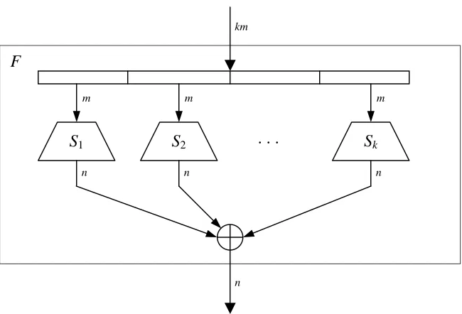
Let F:Ζkm2 →Ζn2 be a transformation such that
F(x) = F(xk, xk–1, …, x1) = S1(x1) ⊕S2(x2) ⊕ … ⊕Sk(xk),
where Si:Ζ2m→Ζ2n, i = 1, 2, ..., k and Si = [fi,n, fi,n–1, ..., fi,1], , :Ζ2 →Ζ2
m j i
Figure 4.1: The structure of F round function.
Similarly to substitution boxes it is defined the nonlinearity of the transformation
n km
F:Ζ2 →Ζ2:
NLF = NLb⋅F
b
min , (4.1) where }b 2 \{0
n Ζ
∈ , b = [bn, bn–1, ..., b1], F = [Fn, Fn–1, ..., F1], :Ζ2 →Ζ2
km j
F ,
Fj(x) = Fj(xk, xk–1, …, x1) = f1, j(x1) ⊕ f2, j(x2) ⊕ ... ⊕ fk, j(xk) and NLb⋅F is nonlinearity of the
Boolean function b⋅F = bnFn⊕bn–1Fn–1⊕ ... ⊕b1F1.
Lemma 4.1 (Piling-Up Lemma, Matsui [6])
Let X1, X2, ..., Xn be independent binary random variables, where n≥ 2 and let
P{Xi = 0} = pi, P{Xi = 1} = 1 – pi for i = 1, 2, ..., n. Then
∏
∏
= −
=
− − = +
+ = = ⊕ ⊕
⊕ n
i i n n
i i n
n p
X X
X
1 1 2 1 1
2 1 1
2 1 2
1 0} 2 ( ) 2
{
P K ε ,
where pi = 21+εi,
2 1 2
1 ≤ ≤
− εi .
Proof (by induction) Let n = 2, then
= − −
+ + +
= − −
+ =
= = =
+ = =
= = =
= ⊕
) )( (
) )( (
) 1 )( 1 (
} 1 , 1 { P } 0 , 0 { P } {
P } 0 {
P
2 2 1 1 2 1 2 2 1 1 2 1 2 1
2 1
2 1
2 1
2 1 2
1
ε ε
ε ε
p p
p p
X X X
X X
X X
X F
km
m m m
S1 S2 . . . Sk
n
). )(
( 2
2 21
2 2 1 1 2 1 2 1 2 1 2 1 1 2 1 2 2 1 4 1 2 1 1 2 1 2 2 1 4 1 − − + = + = = + − − + + + + = p p ε ε ε ε ε ε ε ε ε ε
Let us assume the thesis of the Lemma is true for n = 2, 3, ..., k. Then for n = k + 1 we have
= = = ⊕ ⊕ + = = ⊕ ⊕ = = = ⊕ ⊕ ⊕ + + + } 1 , 1 { P } 0 , 0 { P } 0 { P 1 2 1 1 2 1 1 2 1 k k k k k k X X X X X X X X X X X X K K K = − ⎟⎟ ⎠ ⎞ ⎜⎜ ⎝ ⎛ − + + ⎟⎟ ⎠ ⎞ ⎜⎜ ⎝ ⎛ + = = − ⎟⎟ ⎠ ⎞ ⎜⎜ ⎝ ⎛ − − − + ⎟⎟ ⎠ ⎞ ⎜⎜ ⎝ ⎛ − + = + = − + = − + = − + = −
∏
∏
∏
∏
) ( 2 ) ( 2 ) 1 ( ) ( 2 1 ) ( 2 1 2 1 1 1 2 1 1 2 1 1 1 2 1 1 1 2 1 1 2 1 1 1 2 1 1 2 1 k k i i k k k i i k k k i i k k k i i k p p p p ε ε ε ε . ) ( 2 2 2 2 2 2 1 1 2 1 2 1 1 1 2 1 1 1 1 1 2 1 2 1 4 1 1 1 1 1 2 1 2 1 4 1∏
∏
∏
∏
∏
∏
+ = + = + = − = − + + = − = − + − + = + = = + − − + + + + = k i i k k i i k k i i k k i i k k k i i k k i i k k p ε ε ε ε ε ε εThe calculation above implies that the thesis is true for n≥ 2.
g
The following lemma is a generalization of the result given without proof by Youssef, Chen and Tavares in [11].
Lemma 4.2
∏
= − − − − − ≥ k i S m k kmF NL i
NL 1 1 1 1 ) 2 ( 2 2 . Proof
Let us take the linear approximation of the transformation F :
a⋅x = b⋅F(x), where }a 2 ,b 2 \{0
n
km ∈Ζ
Ζ
∈ , in other words
a1x1⊕a2x2⊕ ... ⊕akxk = bS1(x1) ⊕bS2(x2) ⊕ ... ⊕bSk(xk).
Let pβ denotes the probability of the linear approximation of transformation F having the best efficiency, then by Lemma 3.3 we have km F
km NL p 2 2 1 2
1 = −
− −
β .
where }ai∈Ζm2,bi∈Ζn2 \{0 . Let pγ denotes the probability of generalized approximation having the best efficiency. Then 21
2
1 ≤ −
− γ
β p
p , since in the worst case we can take b1 = b2 = ... = bk = b. Let us transform the generalized approximation to the form
a1x1⊕b1S1(x1) ⊕a2x2⊕b2S2(x2) ⊕ ... ⊕akxk⊕bkSk(xk) = 0.
We assume that Xi = aixi ⊕ biSi(xi) are independent binary random variables having the
probability distribution P{Xi = 0} = pi, P{Xi = 1} = 1 – pi. This assumption is very natural
since pi are the probabilities of linear approximation of independent substitutions boxes Si. By
Lemma 4.1 we have
∏
= − − + = = ⊕ ⊕ ⊕ = k i i k k p X X X p 1 2 1 1 2 1 21 0} 2 ( )
{
P K ,
∏
= − − = − k i i k p p 1 2 1 1 21 2 .
If we take the approximations of substitutions boxes having the best efficiency, which probabilities are equal
k
p p
pβ , β , , β
2
1 K respectively, then
2 1 1 2 1 1
2
∏
− = −= − γ β p p k i i k .
Since 21
2
1 ≤ −
− γ
β p
p , hence
∏
= − − − ≤ − k i i k km F km p NL 1 2 1 1 1 2 2 2 β and consequently
∏
= − + − − − ≥ k i i m k km F p NL 1 2 1 1 ) 1 ( 1 22 β .
By Lemma 3.3 we obtain
= − − = ⎟ ⎟ ⎠ ⎞ ⎜ ⎜ ⎝ ⎛ − − = = ⎟ ⎟ ⎠ ⎞ ⎜ ⎜ ⎝ ⎛ − − = − − ≥
∏
∏
∏
∏
= + − − + − = + − + − = − − + − = − + − k i S m m k m k km k i m S m m k km k i m S m m k km k i i m k km F i i i NL NL NL p NL 1 ) 1 ( 1 ) 1 ( 1 1 1 1 ) 1 ( 1 1 1 1 ) 1 ( 1 1 2 1 1 ) 1 ( 1 ) 2 2 ( 2 2 2 2 2 2 2 2 2 2 2 2 2 β . ) 2 ( 2 2 ) 2 2 ( 2 1 1 1 1 1 2 11
∏
∏
Lemma 4.3 ) )( ( ˆ ) )( ( ˆ ) )( ( ˆ ) )( ( ˆ 2 2 1
1 W S W Sk k
S W F
W b⋅ u = b⋅ u b⋅ u K b⋅ u ,
where u = [uk, uk–1, ..., u1].
Proof
Since b⋅F = bnFn⊕bn–1Fn–1⊕ ... ⊕b1F1 for F = [Fn, Fn–1, ..., F1], :Ζ2 →Ζ2
km j
F ,
Fj(x) = Fj(xk, xk–1, …, x1) = f1, j(x1) ⊕f2, j(x2) ⊕ ... ⊕fk, j(xk),
we have
b⋅F(x) = bnFn(x) ⊕bn–1Fn–1(x) ⊕ ... ⊕b1F1(x) =
= bn( f1,n(x1) ⊕f2,n(x2) ⊕ … ⊕fk,n(xk)) ⊕bn–1( f1,n–1(x1) ⊕f2,n–1(x2) ⊕ … ⊕fk,n–1(xk)) ⊕ ... ⊕
b1( f1,1(x1) ⊕f2,1(x2) ⊕ … ⊕fk,1(xk)) =
= bn f1,n(x1) ⊕bn-1 f1,n–1(x1) ⊕ ... ⊕b1 f1,1(x1) ⊕
⊕bn f2,n(x2) ⊕bn–1 f2,n–1(x2) ⊕ ... ⊕b1 f2,1(x2) ⊕ ... ⊕
⊕bn fk,n(xk) ⊕bn–1 fk,n–1(xk) ⊕ ... ⊕b1 fk,1(xk) = b⋅S1(x1) ⊕b⋅S2(x2) ⊕ ... ⊕b⋅Sk(xk).
Then . ) )( ( ˆ ) )( ( ˆ ) )( ( ˆ ) 1 ( ) 1 ( ) 1 ( ) 1 ( ) 1 ( ) 1 ( ) 1 ( ) 1 ( ) 1 ( ) 1 ( ) 1 ( ) 1 ( ) )( ( ˆ 2 2 1 1 ) ( ) ( ) ( ) ( ) ( ) ( ] ,..., , [ ] ,..., , [ ] ,..., , [ )) ( ... ) ( ) ( ( ) ( 2
1 2 2 2
2 2 2 2 1 1 1 1
2 1 2 1 2
2 2 1 1 2 2 1 1 2 1 1 1 1 1 1 2 2 1 1 2 k k S S S S S S S S S F S W S W S W F W
m m m
k k k k k m
k k m m
k k k k m i k k k k k k k k km u b u b u b u b
x x x
x u x b x u x b x u x b x x x
x u x u x u x b x b x b x x x x x x x x u u u x x x b x x u x b ⋅ ⋅ ⋅ = = − − − − − − = = − − = = − − = − − = ⋅
∑
∑
∑
∑ ∑
∑
∑
∑
Ζ ∈ ∈Ζ ∈Ζ ⋅ ⋅ ⋅ ⋅ ⋅ ⋅ Ζ ∈ ∈Ζ ∈Ζ ⋅ ⊕ ⊕ ⋅ ⊕ ⋅ ⋅ ⊕ ⊕ ⋅ ⊕ ⋅ Ζ ∈ = ⋅ ⊕ ⊕ ⊕ ⋅ Ζ ∈ ⋅ ⋅ − − − − K KK K K
g Theorem 4.4
∏
= ⋅ − − − ⋅ = − − k i S m k kmF NL i
NL 1 1 1 1 ) 2 ( 2 2 b b . Proof
By Lemma 2.4 2 max ˆ( )( )
2 2 1 1 u b u
b W F
NL
km
km
F = − ⋅
Ζ ∈ −
⋅ and by Lemma 4.3
) )( ( ˆ ) )( ( ˆ ) )( ( ˆ ) )( ( ˆ 2 2 1
1 W S W Sk k
S W F
. ) )( ( ˆ max )
)( ( ˆ max ) )( ( ˆ max 2
) )( ( ˆ ) )( ( ˆ ) )( ( ˆ max 2
2 2
2 2
1
1 1 2
2 2 1
1 2
1 1
2 2 1
1 )
, , , ( 2 1 1
k k km
k k km
F
S W S
W S
W
S W S
W S
W NL
m k m
m
k k
km
u b u
b u
b
u b u
b u b
u u
u
u u u u
u b
⋅ ⋅
⋅ −
=
= ⋅
⋅ ⋅
− =
Ζ ∈ Ζ
∈ Ζ
∈ −
= ∈Ζ −
⋅
−
K
K
K
Since 2 max ˆ( )( )
2
2 1 1
u b
u
b i
m
S W S
NL
m i = − ∈Ζ ⋅
−
⋅ , it means m Si
m
i NL
S
W ⋅
Ζ
∈ ⋅ = − b
u
u
b )( ) 2 2
( ˆ max
2
, and consequently
∏
∏
= ⋅
− −
−
= ⋅
−
⋅ = − − = − −
k
i
S m
k km k
i
S m
km
F NL i NL i
NL
1 1 1
1 1
2 1 1
) 2
( 2 2
) 2 2 (
2 b b
b .
g
The above theorem has been used to calculate in the special cases the nonlinearity of the function F according to the formula (4.1).
5 The TGR Algorithm
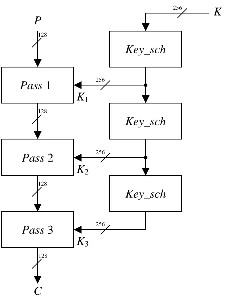
The TGR algorithm is a block cipher which works on 128-bit blocks and uses 256-bit keys. The general scheme of the cipher TGR is shown in the Figure 5.1. The 128-bit plaintext P is transformed to the 128-bit ciphertext C in three passes (r = 1, 2, 3) each consisting of eight rounds ( j = 0, 1, …, 7).
The passes use the 256-bit keys Kr obtained from the main 256-bit key K using the key
schedule algorithm Key_sch. We have Kr = Key_sch(Kr–1), where K0 = K. Each key Kr is
divided into eight 32-bit subkeys kr, j, which are used in the corresponding j-th round of the
r-th pass. The first use of Key_sch has as an input the main key K = (k0, k1, k2, k3, k4, k5, k6, k7) and gives as an output the key K1 = (k1,0, k1,1, k1,2, k1,3, k1,4, k1,5, k1,6, k1,7) used in the first pass. Next we have as an input to Key_sch the key K1 and we get as an output K2 = (k2,0, k2,1, k2,2,
k2,3, k2,4, k2,5, k2,6, k2,7) and analogously for K3 = (k3,0, k3,1, k3,2, k3,3, k3,4, k3,5, k3,6, k3,7). The
Key_sch is described by the formulae shown in Figure 5.2. Operations like + and – are just an addition and a subtraction modulo 232 respectively, ⊕ is a bitwise sum modulo 2, ~ denotes a bitwise negation, << and >> are bitwise shifts left and right respectively (the loosing bits are complemented by zeros), <<< and >>> are bitwise rotations left and right respectively.
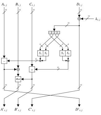
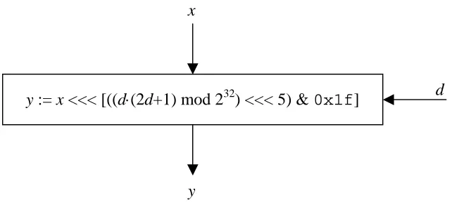
D’r, j). The structure of the round is depicted in the Figure 5.3. The S-boxes S1, S2, S3, S4 are taken from the CAST-256 cipher [2] and operation Rot is the data-dependent rotation function just taken from the RC6 cipher [10] as shown in Figure 5.4.
The TGR design is based on the hash function Tiger proposed by Anderson and Biham in [4].
Figure 5.1. The scheme of the TGR encryption algorithm.
k0 := k0 – (k7⊕ ((~k6) <<< 11) ⊕0xa5a5a5a5)
k1 := k1⊕k0
k2 := k2 + k1
k3 := k3 – (k2⊕ ((~k1) >>> 13))
k4 := k4⊕k3
k5 := k5 + k4
k6 := k6 – (k5⊕ ((~k4) >> 7))
k7 := k7⊕k6
k0 := k0 + k7
k1 := k1 – (k0⊕ ((~k7) << 5)) 256
256 256
P
Pass 1
Pass 2
K
Pass 3
Key_sch
128 128
Key_sch
128
128
C
K1
K3
K2
Key_sch
k4 := k4 – (k3⊕ ((~k2) <<< 11))
k5 := k5⊕k4
k6 := k6 + k5
k7 := k7 – (k6⊕ ((~k5) >>> 13))
k0 := k0⊕k7
k1 := k1 + k0
k2 := k2 – (k1⊕ ((~k0) >> 7))
k3 := k3⊕k2
k4 := k4 + k3
k5 := k5 – (k4⊕ ((~k3) << 5))
k6 := k6⊕k5
k7 := k7 + k6
Figure 5.2. The key schedule algorithm Key_sch.
Figure 5.3. The j-th round of the r-th pass of the encryption algorithm. 32
A’r, j B’r, j C’r, j D’r, j
32
Rot
32 32
32
8 8 8
8
S1 S2 S3 S4
c’3c’2c’1c’0
+
Ar, j Cr, j
–
32
Br, j
32
kr, j
Dr, j
32
32 32 32
Figure 5.4. The data-dependent rotation function Rot.
The TGR decryption algorithm is obtained by taking the inversion of the TGR encryption algorithm (suitable modification of the round function and opposite order of the subkeys).
6 Resistance of TGR to Linear Cryptanalysis
It has been stated in [5] that the best linear approximation of a cipher, satisfied with the probability pL is bounded as follows:
α
β α
2 1 2
2
1 ≤ 1 −
− −
p
pL , (6.1) where α is the number of S-box linear approximations involved in the linear approximation of the cipher and pβ represents the probability of the best S-box linear approximation (among all the α S-box linear approximations). In every round of the block cipher TGR there are involved two 16×32-bit S-boxes each consisting of two 8×32-bit S-boxes taken from the CAST-256. The linear approximation of a block cipher is based on the assumption of independent round keys such that the linear expressions approximating the S-boxes are independent. The sequence of approximations of the round functions (involving approximations of the S-boxes) results in the overall linear expression for the cipher. According to [6] the number of known plaintexts required to almost sure deduction of some bits of the round keys is approximately equal to
2 1−
−
= p
N . (6.2)
y := x <<< [((d⋅(2d+1) mod 232) <<< 5) & 0x1f] d
It was shown in [5] (see Lemma 3.3 above) that the probability pβ is given by m
m
NL p
2 2 2
1 min
1−
=
− −
β , (6.3)
where m is the number of input bits of the S-box and NLmin is minimal nonlinearity of the S-boxes involved in the approximation of the cipher. In our case of TGR cipher we have m = 16 and using Theorem 4.4 we have calculated NLmin being 28736 for the 16×32-bit S-box built from the substitution boxes S1 and S2 taken from the CAST-256 cipher. The best linear approximation of TGR cipher appears to be constructed using two round characteristics when in each round it is approximated the left one 16×32-bit S-box (see Figure 5.3) and the arithmetic addition and subtraction are replaced by xor operation and the data-dependent rotation is neglected. These characteristics are not iterative ones. When calculating (6.3) with our data we obtain
1024 63 2 1
= − β p
and putting α =24 in (6.1) we have
22 10 725545 .
0 2
1 ≤ ⋅ −
− L
p .
From (6.2) we get that the number of required plaintexts to perform the linear cryptanalysis is 147
44
2 10 8996 .
1 ⋅ ≈
≥
p
N
which is much more that the number 2128 of all available plaintexts.
If we perform such analysis, when in each two round characteristic there are approximated two 8×32-bit substitution boxes S1 and S2 having nonlinearity 74, we get that the required number of plaintexts is greater than 2121. It shows that we obtain the better resistance of the cipher to linear cryptanalysis when considering bigger S-boxes in the round function confirming this way the observation made by Youssef et al. in [11].
conclude that TGR algorithm has a one pass (8 rounds) of the security margin with respect to the linear cryptanalysis.
References
[1] C. M. Adams, “Constructing Symmetric Ciphers using the Cast Design Procedure”, Designs, Codes, and Cryptography, vol. 12, no. 3, 1997, pp. 283-316.
[2] C. M. Adams, “The CAST-256 Encryption Algorithm”, available at AES web site: crcs.nist.gov/encryption/aes
[3] N. Ahmed and K. R. Rao, “Orthogonal Transforms for Digital Processing”, Springer-Verlag, 1975.
[4] R. Anderson and E. Biham, “Tiger: New Hash Function”, Third International Workshop, Fast Software Encryption, LNCS 1039, Springer-Verlag, 1996, pp. 89-97.
[5] J. Lee, H. M. Heys and S. E. Tavares, “On the Resistance of the CAST Encryption Algorithm to Differential and Linear Cryptanalysis”, Designs, Codes, and Cryptography, vol. 12, no. 3, 1997, pp. 267-282.
[6] M. Matsui, “Linear Cryptanalysis Method for DES Cipher”, Advances in Cryptology, Proceedings of Eurocrypt ’93, T. Helleseth, Ed., Springer-Verlag, 1994, pp. 386-397. [7] W. Meier and O. Staffelbach, “Nonlinearity Criteria for Cryptographic Functions”, Advances in Cryptology, Proceedings of Eurocrypt ’89, LNCS 434, J. –J. Quisquater and J. Vandewalle, Eds., Springer-Verlag, 1990, pp. 549-562.
[8] K. Nyberg, “Perfect Nonlinear S-Boxes”, Advances in Cryptology, Proceedings of Eurocrypt ’91, LNCS 547, D. W. Davies, Ed., Springer-Verlag, 1991, pp. 378-386. [9] J. Pieprzyk and G. Finkelstein, “Towards Effective Nonlinear Cryptosystem Design”, IEE Proceedings-E, vol. 135, 1988, pp. 325-335.
[10] R. L. Rivest, M. J. B. Robshaw, R. Sidney, and Y. L. Yin, “The RC6 Block Cipher”, available at AES web site: crcs.nist.gov/encryption/aes