GENETICS | INVESTIGATION
Estimating Effective Population Size from
Temporally Spaced Samples with a Novel, Ef
fi
cient
Maximum-Likelihood Algorithm
Tin-Yu J. Hui1and Austin Burt Department of Life Sciences, Silwood Park Campus, Imperial College London, Ascot, Berkshire SL5 7PY, United Kingdom ORCID ID: 0000-0002-1702-803X (T.J.H.)
ABSTRACT The effective population sizeNe is a key parameter in population genetics and evolutionary biology, as it quantifies the
expected distribution of changes in allele frequency due to genetic drift. Several methods of estimatingNehave been described, the most
direct of which uses allele frequencies measured at two or more time points. A new likelihood-based estimatorNcB for contemporary
effective population size using temporal data is developed in this article. The existing likelihood methods are computationally intensive and unable to handle the case when the underlyingNe is large. This article tries to work around this problem by using a hidden Markov
algorithm and applying continuous approximations to allele frequencies and transition probabilities. Extensive simulations are run to evaluate the performance of the proposed estimator NcB;and the results show that it is more accurate and has lower variance than
previous methods. The new estimator also reduces the computational time by at least 1000-fold and relaxes the upper bound ofNeto
several million, hence allowing the estimation of largerNe:Finally, we demonstrate how this algorithm can cope with nonconstantNe
scenarios and be used as a likelihood-ratio test to test for the equality ofNethroughout the sampling horizon. An R package“NB”is now
available for download to implement the method described in this article.
KEYWORDSeffective population size; genetic drift; maximum-likelihood estimation
T
HE effective size of a population is a key concept in pop-ulation genetics that links together such seemingly dispa-rate quantities as the equilibrium levels of genetic variation and linkage disequilibrium, the size of temporal changes in allele frequencies, the probability offixation of a new muta-tion, and others (Charlesworth and Charlesworth 2010). Of-ten Ne is estimated from information on mutation rates and standing levels of nucleotide variation (Charlesworth 2009). In most species there is some level of population differentia-tion (i.e., individuals from geographically distant areas are more genetically different than those from the same loca-tion), and in this case standing levels of genetic variation within a local population give estimates of the effective pop-ulation size summed across all subpoppop-ulations of the species(Charlesworth and Charlesworth 2010). Standing levels of variation also reflect effective population sizes over many thousands or millions of generations.
For some purposes it is more interesting to estimate the current (or recent) size of a local subpopulation. In these cir-cumstances it is common to usefluctuations in allele frequencies over multiple generations to estimate Ne;with larger fluctua-tions indicating a smaller variance effective population size (Krimbas and Tsakas 1971; Waples 1989). This follows from the fact that the variance of genetic drift experienced in a pop-ulation is a function of Ne and can be quantified under the Wright–Fisher model. The variance of genetic drift in one gen-eration ispð12pÞ=ð2NeÞfor a diploid population with effective population size Ne and initial allele frequency p [for haploid populations,pð12pÞ=Ne]. Hence it is possible to estimate the effective population size of a closed population by investigating the magnitude of temporal changes in allele frequencies.
One approach to estimatingNefrom temporal samples is to useF-statistics (Krimbas and Tsakas 1971; Nei and Tajima 1981; Pollak 1983; Waples 1989; Jorde and Ryman 2007).
F-statistics can be obtained by calculating the standardized Copyright © 2015 by the Genetics Society of America
doi: 10.1534/genetics.115.174904
Manuscript received January 25, 2015; accepted for publication February 26, 2015; published Early Online March 5, 2015.
Available freely online through the author-supported open access option.
1Corresponding author: Department of Life Sciences, Silwood Park Campus, Imperial College London, Ascot, Berkshire SL5 7PY, United Kingdom.
variance of gene frequency change, after sampling error is taken into consideration. TheF-statistics are moment-based estimators, making them easy to compute. They tend to be slightly biased upward in general and suffer from large bias when rare alleles are used (Waples 1989; Wang 2001).
Another class of temporal estimators uses the likelihood approach. Williamson and Slatkin (1999) proposed the full-likelihood approach in estimatingNe(see also Andersonet al. 2000; Wang 2001; Berthier et al.2002). There are several advantages of using maximum likelihood over theF-statistics. For example, the maximum-likelihood estimator has a lower variance and smaller bias, resulting in more precise estimates (Williamson and Slatkin 1999; Wang 2001). It also allows a moreflexible sampling scheme, that allele frequency data can be collected from more than two time points. On the downside, the likelihood methods are computationally de-manding compared to the F-statistics, because they make use of the full distributional information of the allele fre-quency across generations. Numerical maximization of the likelihood function is usually involved, and the associated computational difficulties increase with more loci and longer sampling horizons. As a result, the likelihood methods are not suitable for populations with large Ne. TheNe used in pre-vious simulation studies were limited to between 20 and 100 diploid individuals only (Williamson and Slatkin 1999; Andersonet al.2000; Wang 2001; Berthieret al.2002).
It is unfortunate that computing difficulties limit the use of the current likelihood approaches, despite their precision and rigorous statistical basis. Waples (1989) and Pollak (1983) both commented that indirect (genetic) methods for estimat-ingNeare necessary only ifNeis large, but this is precisely the case in which the temporal methods are less reliable. This study aims to provide an alternative likelihood-based estimator that solves the problems in the current likelihood methods. Therefore the new estimator should (1) be computationally compact, (2) be able to work with a wide range of Ne; and (3) be mostly unbiased and have at least the same degree of precision as the other methods.
Theory
The full-likelihood model and MLNE
The full-likelihood model was developed by Williamson and Slatkin (1999) and is used as the basic model in this article. The full-likelihood function for two samples is
LðNeÞ ¼fðx0;xtjNeÞ
¼Xp
0;ptfðx0jp0ÞfðxtjptÞfðptjp0;NeÞfðp0jNeÞ (1)
(Williamson and Slatkin 1999, equation 4), wherex0; xtare the sampled allele counts andp0;ptare the underlying true allele frequencies. For sampling, it is assumed that the sam-ples are taken with replacement; hencefðx0jp0ÞandfðxtjptÞ
are binomially and independently distributed with nbeing the number of sampled diploid individuals:
fðxijpiÞ ¼ 2n! xi!ð2n2xiÞ!
pxii ð12piÞ2n2xi; for i¼0;t: (2)
The probability fðptjp0;NeÞ is calculated using the forward transition matrixM. Each element ofM,fmgij ;is the
prob-ability of the population drifting from the state having i
copies to j copies of an allele. Under the Wright–Fisher model, the transition matrix for biallelic loci can be obtained from a binomial distribution. As the possible number of alleles runs from 0 to 2Ne;the dimension of the transition matrixMis ð2Neþ1Þ3ð2Neþ1Þ: Clearly a computational issue arises here. For a moderately largeNe;sayNe¼10;000;the dimen-sion of the transition matrix becomes 20,0012 (which is 400 million), and this is the number of transition probabilities that needs to be calculated tofill in the matrixM. Furthermore, if the two samples were taken fromtgenerations apart,Mhas to be multiplied by itselfttimes to get the transition probabilities fortgenerations ahead. For largeNeit may not be feasible to compute every element in the matrixMand multiply a matrix of such a size, even with the advance of computing power.
For the likelihood function itself, p0 andpt are nuisance (unobserved, latent state) parameters that need to be mar-ginalized out by summing over all possible combinations of
p0 andpt:For more than two samples, the likelihood func-tion becomes
LðNeÞ ¼fðx0;x1;. . .;xtjNeÞ
¼Xp
0;p1;...;pt
fðx0jp0Þfðx1jp1Þ. . .fðxtjptÞ
3fðptjpt21Þ. . .fðp1jp0;NeÞfðp0jNeÞ
(3)
(Williamson and Slatkin 1999, equation 6), wherep0;p1;. . .;pt are the underlying true allele frequencies and treated as nui-sance parameters. To marginalize out the underlying allele frequencies, we need to sum over all possible values of
p0;p1;. . .;pt;and the number of summations equals the
num-ber of nuisance parameters. Closed-form expressions of the sum-mations may not exist, and they are calculated numerically in this case. Although the form of the likelihood function is explicit, it is computationally intensive to evaluate and maximize it.
While no software appears to be available for the full-likelihood model, the software package MLNE was created to implement the pseudolikelihood approach proposed by Wang (2001) and Wang and Whitlock (2003). The pseudo-likelihood omits some of the insignificant transition proba-bilities in the matrix M and hence reduces computational effort. However, it is still computationally demanding and the computation time increases rapidly with increasing Ne (Wang 2001). Currently, the upper bound forNethat MLNE can handle is38,000 on a 64-bit Windows machine with 16 GB of memory.
A continuous approximation
(1955) derived the complete solution of the differential equa-tion, using the method of moments. The core assumption of the continuous approximation is thatNe is sufficiently large that the moments of the continuous distribution converge to the exact moments. To visualize the model, the process can be represented as a hidden Markov model (Figure 1) (a sim-ilar diagram appeared in Anderson et al. 2000). Here
p0;. . .;ptare the underlying true allele frequencies according
to the Wright–Fisher model, andx0;. . .;xt are observations from the system. We definex0;. . .;xtas allele counts; hence they are positive integers running from 0; . . .; 2n (assum-ing the species is diploid). We aim to derive the joint relation-ship among all the observationsx0;. . .;xt and then infer the parameterNegoverning the process. We investigate the com-ponents in this likelihood and hence derive our estimatorNcB:
As with the Wright–Fisher model, this model also assumes nonoverlapping generations, an isolated population, and con-stant effective population sizeNe:Other genetic forces includ-ing selection and mutation are assumed to be insignificant relative to genetic drift (Waples 1989; Williamson and Slatkin 1999; Wang 2001).
Two samples: In the two-sample model, we assume only
two samplesx0;xtare obtained. In a later section the model is extended to handle multiple sampling events. The likeli-hood function is the joint density of our two observationsx0 andxt is
LðNeÞ ¼fðxt;x0jNeÞ ¼fðxtjx0;NeÞfðx0Þ: (4)
This is the simplest form of the likelihood function for our parameter of interestNe;given our observed values. We can see that x0 is the initial observed allele count and has no relationship withNe:Thereforefðx0Þdoes not play a role in maximizing the likelihood and can be treated as a constant. We can then rewrite the likelihood function as follows:
LðNeÞ}fðxtjx0;NeÞ: (5)
By considering the unobserved nuisance parameters, the likelihood function becomes
LðNeÞ}fðxtjx0;NeÞ ¼Z1
0
Z 1
0 fðxtjptÞfðptjp0;NeÞfðp0jx0Þdptdp0:
(6)
Equation 6 is the continuous analogy of Equation 1, with summations being replaced by integrals. The terms of the likelihood function have the same meaning as in Equation 1:
fðxtjptÞ is the sampling allele counts at generation t,
fðptjp0;NeÞ is the transition probability that plays the same role as the Wright–Fisher matrix in the full-likelihood model, and the last term fðp0jx0Þ is the distribution of initial allele frequency conditioning on the initial observation. The inte-grals are to“sum over”all possible values of the underlying allele frequencies. In the following paragraphs we evaluate each part of the likelihood function and finally derive the general formula for the likelihood function.
The starting allele frequency is unknown in general. We may assumep0is uniformly distributed [equivalent to betað1;1Þ before any observations are taken, because it brings no addi-tional parameters to the system (Williamson and Slatkin 1999). If x0 is sampled binomially from p0 under Equation 2, then by Bayes’ rule, the conditional distribution ofp0jx0 follows a beta distribution (e.g., chap. 7.2.3 in Casella and Berger 2002):
fðp0jx0Þ ¼R1fðx0jp0Þfðp0Þ 0fðx0jp0Þfðp0Þdp0
betaðx0þ1;2n2x0þ1Þ:
(7)
In fact,fðp0jx0Þhas the same role asfðx0jp0Þfðp0jNeÞin the full-likelihood model in Equation 1.
Next, for the transition probabilityfðptjp0;NeÞ;a continu-ous distribution is used to model allele frequency instead of the discrete transition matrix in the full-likelihood model. The probability density function ofptgivenp0under genetic drift is
fðptjp0;NeÞ betaðdp0;dð12p0ÞÞ; (8)
where d is called the “drift parameter” that controls the amount of drift:
d¼ ð121=2NeÞ t
12ð121=2NeÞt: (9)
The drift parameter is a function of Ne and the sampling intervalt. It is derived from the continuous model of genetic drift by Kimura (1955) for sufficiently largeNeand is a pop-ular method to model the change in allele frequency due to genetic drift (Kitakadoet al.2006; Songet al.2006). For the special case oft¼1;dreduces to 2Ne21:
After obtaining the formulas forfðp0jx0Þandfðptjp0;NeÞ; the integral with respect to p0 in the likelihood function (Equation 6) can be calculated in advance. Let us rewrite the likelihood function:
LðNeÞ}
Z 1
0
fðxtjptÞ Z 1
0
fðptjp0;NeÞfðp0jx0Þdp0
dpt:
(10)
The inner integral forms a hierarchical process that p0 is distributed as beta given the initial observation x0 and pt also follows another beta distribution conditioning on p0:
An exact solution may not exist for this type of integral. Here we propose to use another beta distribution to approximate
Figure 1 Hidden Markov model representing the structure of the
pro-cess.p0;. . .;pt is the sequence of true allele frequencies propagating
according to the Wright–Fisher model but they are unobserved.
the integral. The parameters in this new beta distribution can be obtained by matching thefirst two moments:
Z 1
0
fðptjp0;NeÞfðp0jx0Þdp0
beta
a9¼ dðx0þ1Þ 2nþ2þd;b9¼
dð2n2x0þ1Þ 2nþ2þd
:
(11)
The goodness offit of this approximation is examined in the
Appendix.
Thefinal piece of the likelihood function isfðxtjptÞ;which is the sampling allele count given the underlying true allele frequencypt:If the samples are taken with replacement, then it is binomially distributed as described in Equation 2. Now, putting all the elements together, the likelihood function becomes
LðNeÞ}fðxtjx0Þ
¼ Z 1
0
fðxtjptÞfðptjx0;NeÞdpt
¼ Z 1
0
2n!
xt!ð2n2xtÞ!p xt
t ð12ptÞ2n2xt
3 1
Ba9;b9p a921
t ð12ptÞb921dpt
¼ 2n!
xt!ð2n2xtÞ! 1
Ba9;b9 Z 1
0
pxttþa921ð12ptÞ2n2xtþb921dpt
¼ 2n!
xt!ð2n2xtÞ!
Bxtþa9;2n2xtþb9
Ba9;b9 ;
(12)
whereBðÞis a beta function. This integral has a closed-form solution with fðptjx0;NeÞ being a beta distribution and the binomial sampling offðxtjptÞ:The resultant probability mass function is a beta-binomial distribution with three parame-ters: 2n; a9;and b9:We can see from Equations 10 and 12 that the integrals (which play the same role as the summa-tions in the full-likelihood model) can be evaluated separately with either a closed-form expression or an approximate solu-tion, yielding a much simplified likelihood. The relationship between the two samplesx0andxtis now established through a beta-binomial distribution. We defineNcBas the value ofNeat which the likelihood function attains its maximum, condition-ing on the observations. HenceNcB is the maximum-likelihood estimator (MLE) of the parameterNe:For many unlinked loci, the joint likelihood is calculated as the product of each of the individual likelihoods for the loci.
Three or more samples
The likelihood model can be extended to more than two sampling events, as shown in Figure 1. Here we assume samples are taken from successive generations, giving a sequence of observations
x0;x1;...;xt: Similar to equation 4, the likelihood function is the joint density of the observations:
LðNeÞ ¼fðxt;xt21;. . .;x1;x0jNeÞ: (13)
If we let Xi ¼ ðx0;x1;. . .;xiÞ be all the observations up to time i,
LðNeÞ ¼f
xtjXt21 f
xt21jXt22 . . .f
x1jX0 fðx0Þ:
(14)
We prefer Equation 14 because it illustrates the time de-pendency among the observations. Again fðx0Þ contains no information about Ne and can be neglected. By using the same argument as in the two-sample case, each fðxijXi21Þ is a beta-binomial distribution. The parameters within each beta-binomial distribution are functions ofdand the preced-ing observations. The remainpreced-ing question becomes how the parameters in each beta-binomial distribution are obtained. The calculation of the parameters can be generalized by the following four recurring equations,
a9ðiÞ¼
daði21Þ 1þaði21Þþbði21Þþd
b9ðiÞ¼
dbði21Þ 1þaði21Þþbði21Þþd
aðiÞ¼xiþað9iÞ
bðiÞ¼2n2xiþbð9iÞ;
(15)
with initial values
að0Þ¼x0þ1
bð0Þ¼2n2x0þ1;
withiruns from 1;. . .;t:As a result, each of thexi(given all previous observations) follows a beta-binomial distribution, with parameters
fðxijXi21Þ beta-binomialð2n;að9iÞ;b9ðiÞÞ: (16)
Moreover, the underlying allele frequencypigiven all obser-vations up toifollows a beta distribution:
fpijXi
betaðaðiÞ;bðiÞÞ: (17)
Since the sample sizes and time steps are known, the only parameter remaining in the system isNe;the effective pop-ulation size. The whole likelihood function is the product of multiple beta-binomial distributions. Therefore the MLE can be obtained by choosing a value ofNe¼NcBthat maximizes the likelihood function.
Computer Simulations
the existing methods. The MLNE routine (Wang and Whitlock 2003) and the Fc statistic (Nei and Tajima 1981; Waples 1989) were used as benchmarks. In each iteration, we first simulated the allele frequencies with knownNeacrosst gen-erations according to the Wright–Fisher model. Multiple in-dependent biallelic loci were run at a time, and samples were then taken with replacement with a sample size ofndiploid individuals (a total of 2nalleles), as described in Equation 2. Initial allele frequencies were drawn from the uniform distri-bution. The three methods were then applied to produce three estimates. ForNcB;the likelihood function was formed using either Equation 5 or Equation 14, depending on the number of sampling events, and the likelihood function was maximized numerically. The lower and upper bounds for searching for the maxima were taken to be 50 and 107; re-spectively. For MLNE the upper bounds forNewere restricted to 38,000 because of computing limitations.Fcestimates were calculated within the MLNE package. The asymptotic 95% confidence intervals (C.I.) for MLNE andNcBwere also calcu-lated byfinding the range ofNe in which the log-likelihood dropped by 2 units from its maximum value. Simulations were repeated 1000 times for each parameter setting. Simu-lations were run in R (R Core Team 2013).
Summary statistics for the three estimators are shown in Table 1. Ne was chosen to be 1000 or 5000. Sample sizes (per generation) werefixed to be 10% of the true population size. Table 1 shows that all three methods slightly overesti-mated the underlyingNe;whileNcBhad the smallest bias in all cases investigated. In the two-sample scenario there was little difference among the three methods; however,NcB con-sistently had the smallest variance and bias. For three sam-ples, the differences of the three methods became more pronounced so that the likelihood methods (MLNE and c
NB) outperformed their moment-based counterpart in terms of having smaller standard deviation and bias. The standard deviation of Fc-based estimates was often twice that of the likelihood estimates. This result is consistent with the idea
that the likelihood methods are better able to combine data from more than two samples. Within the likelihood family, the mean width of the 95% C.I. was also calculated. The C.I. using NcB is slightly narrower than MLNE given the same significance level, with similar coverage. In short, all the examined scenarios suggested that NcB was superior to the MLNE and Fcestimators.
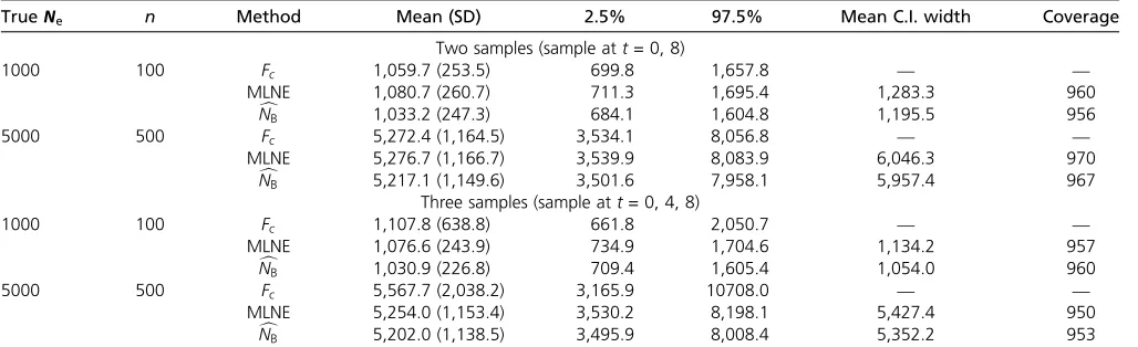
A second set of simulations examined the bias and con-sistency of the new estimator for a range ofNevalues. As the central assumption of the method is that Ne is sufficiently large for a continuous approximation to be valid, it is inter-esting to investigate the performance of theNcBestimator over a wide range ofNe;including small values. A plot of the bias against trueNeis found in Figure 2. For the smaller values of
Ne;NcB slightly underestimated the population size by,2%, while for Ne¼500 and onward NcB was slightly biased up-ward by no more than 2%. This graph supports that NcB is unbiased throughout a wide range of trueNefrom 50. Thus, the new estimator provides an inferential statistic that is not available through prior methods.
NonconstantNe and Likelihood-Ratio Tests
Given three or more samples over time, we can consider the possibility thatNeis different in each sampling interval. This can be done through modifying Equation 15 to allow non-constantd. It is also possible to use the same approach tofit a dynamic model to the data. For example, Wang (2001) demonstratedfitting an exponential growth model with two parameters: initial Neand growth rate. In general, a likeli-hood-ratio test (LRT) can be constructed to compare models and hypotheses. The test statistic is twice the difference in the log-likelihood values under the null and alternative hy-potheses and is asymptotically chi-square distributed with degrees of freedom equal to the difference in the number of parameters between the two models. The following sim-ulated example illustrates how a LRT is constructed.
Table 1 Simulation results
TrueNe n Method Mean (SD) 2.5% 97.5% Mean C.I. width Coverage Two samples (sample att= 0, 8)
1000 100 Fc 1,059.7 (253.5) 699.8 1,657.8 — —
MLNE 1,080.7 (260.7) 711.3 1,695.4 1,283.3 960
c
NB 1,033.2 (247.3) 684.1 1,604.8 1,195.5 956
5000 500 Fc 5,272.4 (1,164.5) 3,534.1 8,056.8 — —
MLNE 5,276.7 (1,166.7) 3,539.9 8,083.9 6,046.3 970
c
NB 5,217.1 (1,149.6) 3,501.6 7,958.1 5,957.4 967
Three samples (sample att= 0, 4, 8)
1000 100 Fc 1,107.8 (638.8) 661.8 2,050.7 — —
MLNE 1,076.6 (243.9) 734.9 1,704.6 1,134.2 957
c
NB 1,030.9 (226.8) 709.4 1,605.4 1,054.0 960
5000 500 Fc 5,567.7 (2,038.2) 3,165.9 10708.0 — —
MLNE 5,254.0 (1,153.4) 3,530.2 8,198.1 5,427.4 950
c
NB 5,202.0 (1,138.5) 3,495.9 8,008.4 5,352.2 953
Consider a three-sample case with samples taken att¼0;4;
and 8, in which we wish to test whetherNeis constant through-out the sampling period. This can be done by setting up the following hypotheses: H0:Ne is constantvs.H1: there are two distinct Ne’s for the period between t¼0 andt¼4 and be-tweent¼4 andt¼8:We canfit two models representing the two hypotheses to the data, one with a singleNeand the other with two differentNe’s. Under the null hypothesis (i.e., given H0 is true), the test statistic asymptotically follows a chi-square distribution with 1 d.f. This can be verified by simulating 5000 replicates as shown in Figure 3.
The statistical power of the test can be exemplified by setting up a specific alternative hypothesis. For example, if the underlying population drops from 10,000 int¼0; 4 to 1000 int¼4; 8;then the power of the test is the probability of rejecting the null hypothesis. There are several parame-ters controlling the power, one of which is the sample size,n
(Figure 4). In the particular example shown, a sample size of
n¼100 is required to attain a power of 80%.
Computational Effort
With the use of the beta and binomial distributions in modeling genetic drift and sampling events, closed-form solutions for the integrals in Equations 11 and 12 are obtained. As a result, the likelihood function (Equation 14) is much simplified and no longer involves summations over all the nuisance parameters as in the full-likelihood model (Equation 1). The comparison of the computation time between MLNE and NcB is shown in Figure 5. For the MLNE package, increases in Ne lead to increases in the number of elements in the transition matrix and therefore in the computing time (Williamson and Slatkin 1999; Wang 2001). ForNcB;continuous approximation is used and the structure of the transition probabilities is approxi-mately the same for allNe:Hence the computing time remains low for any Ne: For both MLNE and NcB; computing time increases with the number of loci used in a similar fashion,
but NcB remains several thousand times faster than MLNE. The speed advantage of NcB also becomes more distinct with increasing sampling interval, becauseNcBdoes not require cal-culation of the power of the transition matrix. It should be noted that the two methods are not coded in the same pro-gramming language (Fortran for MLNE and R forNcB), so these results should not be considered a direct comparison of the two algorithms. However, it likely underestimates the speed advantage of NcB over MLNE because R is a script language, which is typically slower than a compiled language like For-tran. Nevertheless, the new method speeds up estimation by a factor of 1000–10,000 for large Ne without sacrificing accuracy.
Real Example
A real data set from Cuveliers et al. (2011) was used to demonstrate the use of NcB:Six temporal samples spanning
.10 generations were collected between 1957 and 2007 to infer the effective population size of North Sea sole. The sample sizes were 135–220 individuals per generation with 11 microsatellite markers being genotyped. The num-ber of alleles in these loci ranges from 13 to 39. We usedNcB to estimate the overall Ne throughout the entire sampling horizon. The effective population size during the period was estimated to be 2512 with finite 95% confidence limits of 1661 and 4365. The published estimate using MLNE (Wang 2001) was 2169 (C.I. = 1221–5744), while the estimate from the F-statistic (Waples 1989) was 2247 (C.I. = 1127–8370). The complete result can be found in table 2 of Cuvelierset al.
(2011, p. 3561). We found that all three estimates mostly overlap with each other, indicating the consistency among the temporal estimators. The estimate from NcB is slightly larger than those obtained by MLNE and F-statistics, but it is the most precise one with the narrowest confidence interval. c
NBalso showed a significant reduction in computing time; it is 600 times faster than MLNE in this particular example.
Figure 2 Plot of bias of theNcBestimator against trueNe:The bias (solid
line) is quantified as the percentage difference relative to the trueNe: Sample size was 10% of the trueNewith 1000 loci. Two samples were
taken 10 generations apart. The bias approaches 0 (red dotted line) if the estimator is unbiased.
Discussion
The model
In theory, the full-likelihood model (Williamson and Slatkin 1999) for estimating Ne from temporal samples should be the most accurate but is not practical because of computa-tional limitations. MLNE, as a derivation of the full-likelihood model, intentionally omits some of the smaller transition probabilities to enhance computational feasibility. TheNcB es-timator is also an approximation to the full likelihood, but makes use of the continuous approximation to simplify the calculations. Previous studies by Williamson and Slatkin (1999) and Wang (2001) showed that the maximum-likelihood meth-ods are more accurate and precise than theF-statistics, and this article further confirms thatNcBis no exception. The comparison between MLNE andNcBshowed thatNcBis a better alternative to MLNE in a moderately largeNescenario. In our examined cases c
NBproduces a smaller variance and narrower confidence inter-val than MLNE, yielding a more precise estimate ofNe:The bias ofNcBis also negligible, indicating that the approximations hold over a wide range of trueNe:
Perhaps the most important feature of NcB is in relaxing the Ne upper bound. Since the dimension of the Wright– Fisher transition matrix is determined by Ne; MLNE stops the calculation whenNeexceeds a certain value. The current threshold on my workstation is 38,000 while the user manual from MLNE suggests 50,000. This upper bound also applies to the calculation of the upper confidence interval, making the practical range of true Ne even smaller. NcB relaxes this bound to over several million without causing computational issues. As a result, precise estimation of con-temporary Necan be applied to more species. Another dis-tinct advantage is the computing speed, which is increased by a factor of$1000 in most scenarios. Most calculations in c
NBare done within seconds. Field biologists may not appre-ciate this improvement as most of their time is spent on data collection; however, with the anticipated advance in DNA se-quencing technology, large amounts of loci can be sequenced at a time with low cost. The ability of existing software to handle
such a data set is questionable. Furthermore, with the increas-ing popularity of the use of computer simulation in population genetics (such asmsby Hudson 2002), in which the computing time is multiplied by the number of repeated simulations,NcB provides an efficient algorithm to help scientists evaluate their simulations rapidly and accurately.
Usage
As discussed above,NcBis designed for moderately largeNe populations and this explains why our simulations focused
Figure 4 Statistical power against sample size. A specific H1was chosen as described in the text, with 1000 independent loci.
Figure 5 Comparison of computational effort (in seconds) between
MLNE and cNB:A shows the computational time against trueNe:Ne of
in these scenarios. Although we showed thatNcBis unbiased even for small values ofNe;we suggest using the full-likelihood method for the extremely smallNeproblem (whenNe,100). In determining sample size, it has to be viewed relative to the trueNeof the population. It is shown in our simulations that sampling 10% of the individuals is able to estimateNe accu-rately, with the use of 500 independent loci. Interested readers can refer to Waples (1989) and Wang (2001) for more details about the effect of sampling effort on temporal methods.
Excluding rare alleles is not unusual in population genetics studies. For instance, LDNE (Waples and Do 2008) imposes several cutoffs for rare alleles. Wang (2001) showed that the moment-based F-statistics induces bias with rare alleles, while the likelihood methods are less sensitive to small allele fre-quency as they make use of the full distributional information of the Wright–Fisher model. We analyzed empirically the goodness of fit of the beta distribution in modeling allele frequency in theAppendix. We showed that the approxima-tion is indistinguishable from the true continuous model when frequent alleles are used, and it still holds when the observed allele frequency is down to0.05. As a result we suggest that in most cases it is safe to include alleles with observed allele frequency.5%.
In the review by Luikartet al.(2010) they emphasized the desirability of developing new methods that are able to distin-guish between moderate and largeNe and that future devel-opment ofNeestimators should allow for the possibility of genotyping many loci. The methods developed here allow for expansion in these two directions, both for estimating effective population sizes and for testing for significant dif-ferences (or trends) in population sizes from temporally spaced samples.
R package
An R package “NB” has been created to implement NcB as described in this article. The package allows moreflexibility, including unevenly temporal-spaced samples and noncon-stant sample size. As demonstrated in our worked example, multiallelic loci are accepted in the R package through the use of Dirichlet-multinomial distribution. It also contains a sample data set and a help document to describe the usage of the package. It is available for download at http://cran.r-project.org/web/packages/NB/.
Acknowledgments
We thank Tony Nolan, Dan Reuman, and Jinliang Wang for useful discussions. This work was funded by a grant from the Foundation for the National Institutes of Health through the Vector-Based Control of Transmission: Discovery Research program of the Grand Challenges in Global Health initiative of the Bill and Melinda Gates Foundation.
Literature Cited
Anderson, E. C., E. G. Williamson, and E. A. Thompson, 2000 Monte Carlo evaluation of the likelihood for Nefrom temporally spaced
samples. Genetics 156: 2109–2118.
Berthier, P., M. A. Beaumont, J. M. Cornuet, and G. Luikart, 2002 Likelihood-based estimation of the effective population size using temporal changes in allele frequencies: a genealogical approach. Genetics 160: 741–751.
Casella, G., and R. L. Berger, 2002 Statistical Inference. Thomson Learning, California.
Charlesworth, B., 2009 Effective population size and patterns of molecular evolution and variation. Nat. Rev. Genet. 10: 195–205. Charlesworth, B., and D. Charlesworth, 2010 Elements of
Evolu-tionary Genetics. Roberts and Co, Colorado.
Cuveliers, E. L., F. A. M. Volckaert, A. D. Rijnsdorp, M. H. D. Larmuseau, and G. E. Maes, 2011 Temporal genetic stability and high effective population size despitefisheries-induced life-history trait evolution in the North Sea sole. Mol. Ecol. 20: 3555–3568.
Fisher, R. A., 1922 Proc. R. Soc. Edinb., 1922, Vol. 42, pp. 321–341. Hudson, R. R., 2002 Generating samples under a Wright-Fisher neutral model of genetic variation. Bioinformatics 18: 337–338. Jorde, P. E., and N. Ryman, 2007 Unbiased estimator for genetic
drift and effective population size. Genetics 177: 927–935. Kimura, M., 1955 Solution of a process of random genetic drift
with a continuous model. Proc. Natl. Acad. Sci. USA 41: 144–150. Kitakado, T., S. Kitada, Y. Obata, and H. Kishino, 2006 Simultaneous estimation of mixing rates and genetic drift under successive sam-pling of genetic markers with application to the mud crab (Scylla paramamosain) in Japan. Genetics 173: 2063–2072.
Krimbas, C. B., and S. Tsakas, 1971 Genetics of dacus-oleae. 5. Changes of esterase polymorphism in a natural population fol-lowing insecticide control-selection or drift. Evolution 25: 454. Luikart, G., N. Ryman, D. A. Tallmon, M. K. Schwartz, and F. W. Allendorf, 2010 Estimation of census and effective population sizes: the increasing usefulness of DNA-based approaches. Con-serv. Genet. 11: 355–373.
Nei, M., and F. Tajima, 1981 Genetic drift and estimation of ef-fective population-size. Genetics 98: 625–640.
Pollak, E., 1983 A new method for estimating the effective population-size from allele frequency changes. Genetics 104: 531–548. R Core Team, 2013 R: A Language and Environment for Statistical
Computing. R Foundation for Statistical Computing, Vienna. Song, S., D. Dey, and K. Holsinger, 2006 Differentiation among
populations with migration, mutation, and drift: Implications for genetic inference. Evolution 60: 1–12.
Wang, J. L., 2001 A pseudo-likelihood method for estimating ef-fective population size from temporally spaced samples. Genet. Res. 78: 243–257.
Wang, J. L., and M. C. Whitlock, 2003 Estimating effective pop-ulation size and migration rates from genetic samples over space and time. Genetics 163: 429–446.
Waples, R. S., 1989 A generalized-approach for estimating effec-tive population-size from temporal changes in allele frequency. Genetics 121: 379–391.
Waples, R. S., and C. Do, 2008 LDNE: a program for estimating effective population size from data on linkage disequilibrium. Mol. Ecol. Resour. 8: 753–756.
Williamson, E. G., and M. Slatkin, 1999 Using maximum likeli-hood to estimate population size from temporal changes in al-lele frequencies. Genetics 152: 755–761.
Appendix
Since the approximation stated in Equation 8 is one of the several key ideas in this article to speed up the current estimation ofNe;it is essential to evaluate how good the approximation is. Equation 8 in the main text is
Z 1
0
fðptjp0;NeÞfðp0jx0Þdp0
beta
a9¼ dðx0þ1Þ 2nþ2þd; b9¼
dð2n2x0þ1Þ 2nþ2þd
:
The left-hand side of Equation 8 is considered as a hierarchical relationship, thatptis distributed as beta given a value ofp0;whilep0 itself is also distributed as beta conditioning on the initial observed countx0(which is afixed value). Two sources of randomness are involved and the integral sums over all possible values of the intermediatep0:However, this kind of integration seldom has an analytical solution. In this article we suggest that this integral can be well approximated by another beta distribution, as suggested in Equation 8.
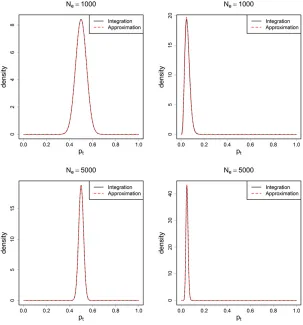
We examined how close the approximation is to the actual integral. Two values ofNewere studied: 1000 and 5000, with eight generations between the two samples taken. Sample size was set to 10% of the trueNe:Under these settings, both low allele frequency (0.1) and even allele frequency (0.5) scenarios were tested. Plots of the results can be found in Figure A1. From the plots we can see that the two lines representing the two methods overlap with each other and are visually indistinguishable. This indicates that in moderately largeNethe use of a beta distribution is a good approximation to the integral. Furthermore, the approximation holds for a wide range of allele frequencies, including the cases where rare alleles are used.
Figure A1 The plots of the conditional density ptjx0;
whereNewas set to be 1000 (top row) and 5000 (bottom
row). Sample size was 10% of the trueNeper generation.