Improved I/O-efficient algorithms for solving graph connectivity, biconnectivity problems.

University of Windsor University of Windsor

Scholarship at UWindsor

Scholarship at UWindsor

Electronic Theses and Dissertations Theses, Dissertations, and Major Papers

1-1-2007

Improved I/O-efficient algorithms for solving graph connectivity,

Improved I/O-efficient algorithms for solving graph connectivity,

biconnectivity problems.

biconnectivity problems.

Shan Li

University of Windsor

Follow this and additional works at: https://scholar.uwindsor.ca/etd

Recommended Citation Recommended Citation

Li, Shan, "Improved I/O-efficient algorithms for solving graph connectivity, biconnectivity problems." (2007). Electronic Theses and Dissertations. 6994.

https://scholar.uwindsor.ca/etd/6994

Im p ro v ed I/O -E ffic ie n t A lg o r ith m s for S o lv in g G raph

C o n n e c tiv ity , B ic o n n e c tiv ity P ro b lem s

by

Shan Li

A Thesis

Submitted to the Faculty of Graduate Studies through Computer Science

in Partial Fulfillment of the Requirements for the Degree of Master of Science at the

University of Windsor

Windsor, Ontario, Canada 2007

Library and Archives Canada

Bibliotheque et Archives Canada

Published Heritage Branch

395 W ellington Street Ottawa ON K1A 0N4 Canada

Your file Votre reference ISBN: 978-0-494-35019-5 Our file Notre reference ISBN: 978-0-494-35019-5

Direction du

Patrimoine de I'edition

395, rue W ellington Ottawa ON K1A 0N4 Canada

NOTICE:

The author has granted a non­ exclusive license allowing Library and Archives Canada to reproduce, publish, archive, preserve, conserve, communicate to the public by

telecommunication or on the Internet, loan, distribute and sell theses

worldwide, for commercial or non­ commercial purposes, in microform, paper, electronic and/or any other formats.

AVIS:

L'auteur a accorde une licence non exclusive permettant a la Bibliotheque et Archives Canada de reproduire, publier, archiver,

sauvegarder, conserver, transmettre au public par telecommunication ou par I'lnternet, preter, distribuer et vendre des theses partout dans le monde, a des fins commerciales ou autres, sur support microforme, papier, electronique et/ou autres formats.

The author retains copyright ownership and moral rights in this thesis. Neither the thesis nor substantial extracts from it may be printed or otherwise reproduced without the author's permission.

L'auteur conserve la propriete du droit d'auteur et des droits moraux qui protege cette these. Ni la these ni des extraits substantiels de celle-ci ne doivent etre imprimes ou autrement reproduits sans son autorisation.

In compliance with the Canadian Privacy Act some supporting forms may have been removed from this thesis.

While these forms may be included in the document page count,

their removal does not represent any loss of content from the thesis.

Conformement a la loi canadienne sur la protection de la vie privee, quelques formulaires secondaires ont ete enleves de cette these.

A bstract

Many large-scale applications involve data sets th at are too massive to fit into the main memory. As a result, some of the data sets must be stored in external memory. Algorithms manipulating these data sets must transfer data between the internal and external memory using I/O (Input/O utput) operations. Consequently, a computational model, called the external memory model, have thus been proposed for these applications. The efficiency of an algorithm in the model is measured in terms of the number of 1/O operations performed.

In this thesis, we present I/O-efficient algorithms for solving the graph connectiv­ ity and biconnectivity problems. Previously best-known external-memory algorithms for the problems are based on simulation of their corresponding Parallel RAM algo­ rithms. By contrast, our algorithms are based on depth-first search and Tarjan’s sequential biconnected-component algorithm. All of our algorithms require 0 (|" |F |/M ] scan(|A|) + |V|) I/Os, where V is the vertex set, E is the edge set and |V| (\E\, respectively) denotes the cardinality of V (E, respectively) in G, M is the size of the internal memory (main memory). For the cases in which [|V |/M ] = 0(1) (i.e. the vertex set size is a constant factor larger than the main memory size) and l-E) > D B \V \ (which includes dense graphs as special cases), where D is the number of disk drives and B is the block size, our exter­ nal memory algorithms require only 0 (scan(A)) I/O s, whereas the previously best-known

D edication

To my parents

Acknow ledgm ents

I would like to express my deepest appreciation to all those who have helped me to complete this research work.

I am greatly indebted to my supervisor Prof. Dr. Yung H. Tsin from the School of Computer Science, who has taught me how to do research and has given me invaluable suggestions and stimulating encouragement in all the time of research and writing of this thesis. This work could not have been completed if it were not for the constant assistance and the professional guidance provided by Prof. Dr. Yung H. Tsin.

I would like to express my great gratitude to Prof. Dr. Tim Traynor, Department of Mathematics and Statistics and Prof. Dr. Richard A. Frost, School of Computer Science for giving me corrections and constructive criticism to improve the quality of the thesis and for being in the committee, and to Prof. Dr. Xiaobu Yuan for serving as the chair of the defense.

My colleagues and all the faculty members and staff of the School of Computer Science have been extremely hospitable in providing their suggestions and their support during the mammoth research work. In particular, Mr. Aniss Zakaria has friendily supplied me with technical support and Ms. Mandy Dumouchelle has given me helpful hands in many day-to-day matters. Many thanks go to Ms. Lihua Duan and Ms. Lin Lan for their help in the successful completion of this work.

There are a few people who have reviewed the thesis from outside the School of Com­ puter Science. Especially, I would like to give my thanks to the staff members of the Academic Writing Center for proof-reading the thesis.

Furthermore, I acknowledge the financial support of my supervisor,’ Prof. Dr. Yung H. Tsin, in the form of research assistantship through NSERC, the School of Computer Science in the form of graduate assistantship, and the Faculty of Graduate Studies and Research in the form of Tuition Scholarship during the entire period of my study at University of Windsor.

C ontents

A b s tra c t 3

D e d ic a tio n 4

A ck n o w led g m en ts 5

L ist o f F ig u re s 8

L ist o f A lg o rith m s 9

1 In tr o d u c tio n 10

1.1 M otivation... 10

1.2 Existing A lgorithm s... 13

1.3 C ontribution... 14

1.4 Organization of T h e s i s ... 15

2 B ac k g ro u n d In fo rm a tio n , 16 2.1 Graph C onnectivity... 16

2.1.1 D efinitions... 16

2.1.2 Depth First S e a r c h ... 18

2.1.3 Tarjan’s Sequential Biconnectivity Algorithm ... 20

2.1.4 The PRAM Biconnected Component A lg o rith m ... 23

2.2 Model of C o m p u ta tio n ... 27

3 R ev iew o f th e C u rre n t S ta te o f th e A rt 29 3.1 The Existing EM Graph-Connectivity A lgorithm ... 31

3.1.1 A Description of the A lg o rith m ... 31

3.2 The Existing EM Biconnectivity A lgorithm ... 33

3.2.1 A Description of the A lg o rith m ... 33

3.3 An Existing EM Depth-first Search A lg o rith m ... 35

3.3.1 A Detailed Description of the A lg o rith m ... 36

3.3.3 Time Complexity A n a ly sis... 42

4 A n E x te rn a l-M e m o ry A lg o rith m for G ra p h C o n n e c tiv ity 44 4.1 A Detailed Description of the A lg o rith m ... 44

4.2 Correctness P r o o f ... 46

4.3 Time C o m p le x ity ... 47

5 A n E x te rn a l-M e m o ry A lg o rith m for B ic o n n e c tiv ity 49 5.1 An EM Algorithm for Detecting Cut-Vertices ...49

5.1.1 Input D ata S t r u c t u r e s ... 49

5.1.2 Computing L O W P O IN T ... 50

5.1.3 Correctness Proof ... 55

5.1.4 Time Complexity A n a ly sis... 57

5.1.5 Detecting the c u t-v e rtic e s ... . ' ... 58

5.2 An EM Algorithm for Detecting Biconnected C o m p o n e n ts ... 59

5.2.1 The Description of EM _BCC... 60

5.2.2 Correctness P r o o f ... 63

5.2.3 Time Complexity A n a ly sis... 64

6 C o m p a riso n o f T im e C o m p le x itie s 6 6

7 C o n clu sio n s 69

List o f Figures

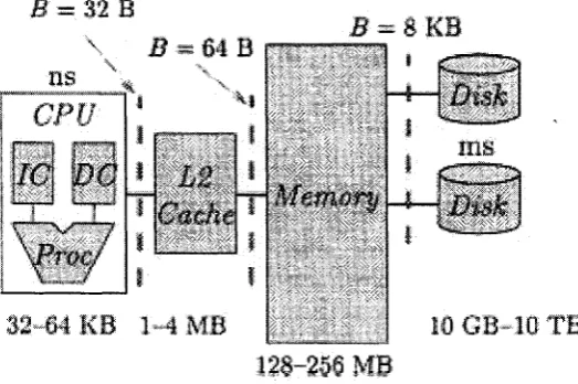
1.1 “The memory hierarchy of a typical uniprocessor system, including regis­ ters, level 1 cache, level 2 cache, internal memory, and disks. Below each memory level is the range of size for this level. Each value of B at the top of the figure is the size of block switched between adjacent levels of this

hierarchy.” [45] p. 211 ... 11

1.2 P latter of a magnetic disk driver [45] p. 2 1 4 ... 12

2 . 1 An example of cut-vertex (articulation point) v2... 17

2.2 After the cut-vertex v2 is removed... 17

2.3 A graph on which a depth-first search is to be performed... 19

2.4 A depth-first search tree. The search starts at the vertex b, an arrow denotes a tree edge leading from parent to child; a dash line denotes a back-edge... 2 0 2.5 The depth-first tree produced by Tarjan’s algorithm for the graph of Figure 2 . 3 21

2.6 An illustration of the graph G' of the relation R c. Figure (a) presents a graph G, including a spanning tree T shown in solid lines with the remain­ ing nontree edges shown in dashed lines. Figure (b) presents the connected components of G' th at are the biconnected components of the graph G shown in (a). [23] p. 2 3 1 ... 24

2.7 (a) A spanning tree represented by solid lines and the dashed edges are nontree edges, (b) The connected components of G' correspond to the biconnected components of G (a). The relation R'c defined by the three conditions. Condition 1: (e4, ei); (e5, e2); Condition 2: (e3,6 4); (e4, e5); Condition 3: (e9,e 10). [23] p. 235 ... 26

List o f A lgorithm s

1 Depth First s e a r c h ... 19

2 Tarjan’s Sequential Biconnected-Component A lg o rith m ... 22

3 The PRAM Biconnected Component A lg o rith m ... 25

4 The EM_GCC algorithm of Chiang et al... 32

5 The EM_BCC Algorithm of Chiang et al... 34

6 Routine R o o te d -T re e ... 35

7 EM Evaluate_Tree... 35

8 A lg o rith m EM_DFS of Chiang et al... 38

9 R o u tin e Unvisited-vertex: To make an unvisited vertex the current vertex 39 10 R o u tin e Compact-array A ... 40

11 A lg o rith m E M _ G C ... 45

12 R o u tin e E M _G C C ... : ... 45

13 R o u tin e U nvisited-vertex... 45

14 R o u tin e Compact-array A ... 46

15 Algorithm LOWPOINT ... 52

16 Encounter an unvisited v e r t e x ... 53

17 Compact the array A when In te r Struct is f u l l ... 54

18 Algorithm EM_BCC ... 61

19 R o u tin e U n v isite d -v e rte x : Encounter an unvisited v e r te x ... 62

20 Compact the array A when In te r Struct is f u l l ... 62

Chapter 1

Introduction

1.1

M o tiv a tio n

D ata sets in large-scale applications are often too massive to fit into the main memory. As a result, traditional RAM algorithms are unsuitable for such large applications owing to the substantial Input/O utput cost. This is because in designing a RAM algorithm, one assumes th at memory access and CPU operation have uniform cost. Unfortunately, this is not the case in large-scale applications. For economical reasons, the memory system of a modern computer consists of a hierarchal structure with distinct access time for the different levels. The highest level, which consists of external disks, is the slowest but has the largest storage size. The lowest level which consists of the registers in the CPU is the fastest but has the smallest storage size. Figure 1.1 shows the memory architecture. In the figure, 8K B is the block transfer size between internal memory and external disks.

For large-scale applications th at have to store partial data sets on external disks, com­ munication between the faster internal memory and the slower external memory is often considered to be the major bottleneck of the computation. This is because the internal memory is many order of magnitude faster than the external disks. Figurel.2 shows the characteristics of a disk. External disks consist of platters of disks and a read/w rite head for locating each platter surface. Each disk stores data sets on concentric circles called tracks. At any time, the read/w rite head has to mechanically locate the correct track to retrieve/transfer data. The location time from one random track to another is often in the order of 3 to 10 milliseconds, compared to the order of nanosecond (10~ 9 seconds) for

accessing internal memory [45].

disk transfer speed. Recently, the gap has been getting larger: developments in technol­ ogy, such as parallel computing, have increased the CPU speed at an annual growth of 40 to 60 percent while the disk transfer speed has only been improved by 7 to 10 percent annually [37]. Consequently, there has been an urgent need to design algorithms that have minimal I/O costs in large-scale computations.

A theoretical computational model, called the external memory model, had been pro­ posed for designing I/O-efficient algorithms (also called external-memory algorithms or EM algorithms). From the perspective of the design of algorithms, minimizing the I/O costs is equivalent to exploiting maximal data locality in the main memory. At the early stage of the development of external memory algorithms, Aggarwal and Jeffrey [2] pro­

posed a standard two-level external memory model. It consists of one logical disk and an internal (main) memory. Later, an improved computational model with multiple logical disks was introduced, which exploits accessing multiple disks in parallel to maximize data locality. It is called the Parallel Disk Model (PDM) [46].

In the PDM model, an I/O operation transfers a block of D B data units between external disks and main memory, or vice versa. At any time, D disks can be accessed in parallel, and each disk can access B records, which are stored in consecutive locations on

32 B

ns

CPU

in s

32-64 KB

MB

10 GB

128-256 MB

the disk. The performance measure for external-memory (EM) algorithms is the number of Input/O utput (I/O ) operations performed to transfer data between the two levels of memory without taking internal computation time into consideration. The following parameters are frequently used in analyzing the I/O complexity of EM algorithms [46]:

scan(N ) = The number of I/O operations needed to read N data records stored on

D disks each with a buffer size B.

sort (a:) = log at The number of I/O operations needed to sort N data records stored across D disks each with a buffer size B.

In the area of graph algorithms, substantial effort has been put into solving large- scale graph problems arising in geographic information systems and web modelling where the data volumes are measured in petabytes (101 5 bytes). For example, data structures

that support external-memory graph algorithms in constructing minimum spanning trees, breadth-first search, depth-first search, and finding single-source shortest paths are pre­ sented in [29]; several new techniques, such as PRAM simulation and time-forward pro­ cessing for graph problems, have been developed in [13]; a large number of fundamental graph problems have been solved efficiently [2, 46, 34, 22, 1, 21], and a number of external- memory algorithms have been proposed for planar graphs [5, 6, 7, 8].

Chiang et al. [13] have shown th at a PRAM algorithm that runs in time T using N

processors and O (N ) space can be simulated in the EM model using 0 ( T *sort(Ar)) I/Os. Many external-memory graph algorithms have thus been derived from the correspond­ ing PRAM algorithms. We observed th at the simulated PRAM algorithms are limited

magnetic surface

disk ©f disk

by sequential access to the disks, and are usually very complicated and are difficult to understand and code.

1.2

E x is tin g A lg o r ith m s

Graph connectivity, which is one of the fundamental graph-theoretic properties, measures the extent to which a graph is connected. In real-life applications, the property represents the reliability of a telecommunication network or a transportation system. Determining biconnectivity is one of the graph connectivity problems which is related to our work. It is a problem th at has been extensively studied on different computational models.

The first biconnectivity algorithm was presented by Tarjan to run on the RAM (the standard sequential computer model). It runs in optimal 0(|R|-|-|£^|) time for a connected graph G = (V, E) [39]. Later on, a number of biconnectivity algorithms were developed for the PRAM (the standard parallel computer model). Typically, Tsin and Chin [42] de­ signed an optimal algorithm for dense graphs on the CREW (concurrent-read-exclusive- write) PRAM th at runs in 0(log2(|E |)) time using 0 (\V \2 / log2(|V” | ) ) 1 processors; Tarjan

and Vishkin [40] developed an algorithm th at takes 0(log(|V j)) time with 0 (\V \ + |E |) processors on the CRCW (concurrent-read-concurrent-write) PRAM. On the distributed computer model, a number of algorithms th at run in 0 (|R |) time and transm its 0 (\E \)

messages of 0(log |C|) length had been proposed [4, 20, 27, 36, 38]. In the fault-tolerance setting, with the assumption that a breadth-first search or depth-first search spanning tree is available, K araata [25] presented a self-stabilizing algorithm th at finds all the bicon­ nected components in 0 (d) rounds (d is the diameter of the graph) using 0 (|R |A lo g A) bits per processor; Devismes [15] improved the bounds to 0 (H ) moves (H is the height of the spanning tree) and 0 (\V \ log A) bits per processor, and Tsin [41] further improved the result to 0 (d n log A) rounds and 0 (|V jlo g A ) bits per processor without assuming the existence of any spanning tree. In wireless sensor network, Turau [43] presented an algorithm th at takes 0 (|Vj) time and transmits at most 4m messages.

In the EM model, Chiang et al. presented the first I/O-efficient biconnected component algorithm. The algorithm is an adaption of the biconnected component PRAM algorithm of Tarjan et al. [13] based on simulation. The EM algorithm performs 0(m in{sort(E 2),

\og(V/M ) sort(E)}) I/O s. Chiang et al. also presented an 0 (\og(V /M ) sort(E')) con­

nected component algorithm [13]. This I/O bound was achieved later on by Abello et al. [1] using a functional approach. Furthermore, they introduced the semi-external model (|Vj < M < [Al). V itter observed th at several graph problems can be solved optimally on this model. For example, finding connected component, biconnected component can be done in 0(scan(A )) I/O s [45]. Subsequently, an I/O complexity, 0 ( { E /V ) sort(F ) • max{ 1, log log( | V j D B/ 1A j)}), for the EM connected component algorithm was reported

by Munagala et al. [34]. Ulrich Meyer pointed out th at the I/O bound of the EM bi­ connected component algorithm of Chiang et al. can be improved to 0 ( ( E /V ) sort(U) • m ax{l, loglog(|U |A £/|A [)}) using the EM connected component algorithm of Munagala

et al. [33]. A lower bound of 0 (|A |/|U | • sort(|U j))I/O s for finding connected components, biconnected components and minimum spanning forests was proved by Munagala and Ranade [34]. Note th at (|A |/|U | • sort(|U |)) = 0(sort(|A |)).

1.3

C o n tr ib u tio n

In this thesis, we design I/O-efficient algorithms for the external-memory model with par­ allel disks (PDM [46]). We shall present I/O-efficient algorithms for both the connected component and biconnected component problems. Since detecting the cut-vertices plays a key role in determining the biconnected components, we shall first present an EM al­ gorithm (called EM_CV) for detecting all the cut-vertices. We then present an algorithm (called EM_BCC) to generate all the biconnected components based on the cut-vertices. Our algorithms for solving the biconnectivity problem are adaptations of Tarjan’s sequen­ tial algorithm. Since the sequential algorithm is developed based on depth-first search, our algorithms are therefore based on the EM depth-first search algorithm of Chiang et al. [13].

In terms of I/O complexity, our algorithms make an improvement over the existing algorithm for dense graphs under certain conditions. The algorithm of Chiang et al. [13] performs 0 (s o rt( |l/|2)) I/O s for dense graphs (i.e. \E\ = 0 (\V \2)) while our algorithm performs 0 { { \\V \/M \) scan(|E|)) I/Os. When \V/M~\ = 0(1) (this includes the semi-external model as a special case), our algorithm performs 0(scan(|V |2)) I/O s on dense graphs which is better than 0 (sort(|C |2)).

1.4

O rg a n iza tio n o f T h e sis

Chapter 2

Background Inform ation

2.1

G rap h C o n n e c tiv ity

The notion of &-vertex-connectivity and fc-edge-connectivity are introduced to measure the extent to which a graph is connected. The larger the value of k, the more connected the graph. In telecommunication systems and transportation networks, these properties represent the reliability of the network in the presence of vertex or link failures. A graph is

k -v ertex -co n n ected (k-edge-connected, respectively) if removing fewer than k vertices (edges, respectively) would not result in a disconnected graph. A bi-con n ected graph is a 2 -v ertex -co n n ected graph. A b ridge-con n ected graph is a 2 -edge-con n ected

graph.

2.1.1

D efin ition s

We shall denote a graph with G = (V ,E), where V = {fi, t’2, ..., v\v\} is the vertex set and E = {ei, e-i,..., e\E\} is the edge set. Each edge e is associated with a pair of vertices

{u, v}. The vertices u and v are called the en d p o in ts of edge e which may be identical. Edge e is in c id e n t to vertex u and v.

D e fin itio n 2 .1 . 1 D irec te d G raph. A directed graph is a graph in which every edge

(called an arc) is associated with an ordered pair of vertices. We shall use < u ,v > to represent an ordered pair.

D e fin itio n 2 .1 . 2 A n u n d ire c te d g ra p h is a graph in which every edge is associated

with an unordered pair of vertices. We shall use (u, v ) to represent an unordered pair.

D efin itio n 2.1.3 P a th . A sequence of vertices, v\, v^, . . . , Vk, is a path if and only if {vi,Vi+\} E E, 1 < i < k. It is called a v\ — Vk path. The path is a c irc u it if v\ = v^. The path is sim p le if every Vi is distinct; the path is a cycle if vi, u2, . . . , Vk- 1 is a simple

D efin itio n 2.1.4 A graph G = (V,E) is a con n ected graph if it has a v — u path, Mv, u e V .

D e fin itio n 2.1.5 B rid g e (o r C u t-edge). In a connected graph G — (V ,E), a bridge is an edge e £ E whose removal leads to a disconnected graph.

D efin itio n 2 .1 . 6 A rtic u la tio n P o in t (o r C u t-v e rte x ). In a connected graph G =

(y,E),

V

2 * i <’5

ih

4 V<3

Vi

Figure 2.1: An example of cut-vertex (articulation point) v2.

Figure 2.2: After the cut-vertex v2 is removed.

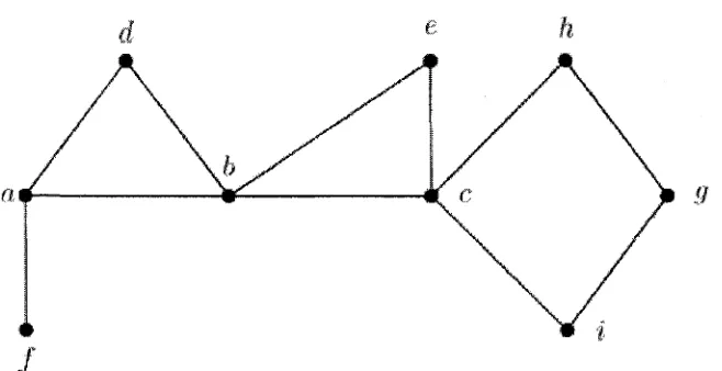
An articulation point is illustrated in Figure 2.1. Vertex v2 is an articulation point because its removal results in a graph having two connected components (see Figure 2.2).

D efin itio n 2.1.7 Subgraph. A graph G' = (V E ' ) is a subgraph of a graph G = (V, E) i f V ' C V and E ' C E .

D efin itio n 2.1.8 B ic o n n e c ted C om pon en t. A biconnected component of G, denoted by Gc = (V c ,E c), is a maximal biconnected subgraph of G.

D e fin itio n 2 .1 . 1 0 Span n in g Tree. A spanning tree T = (V t , E t ) of a graph G =

(V, E) is a subgraph of G such that VF = V. E t Q E and T is a tree. A n edge e of G is a tree edge (w.r.t. T ) if e G E t and is a n o n tree edge (w.r.t. T ) if e6 E — E

t-D efin itio n 2.1.11 Let u be a vertex lying on the path connecting the root r with a vertex v in a tree T. Then u is called an a n c e sto r o fv while v is a d escen d a n t ofu. I f u ^ v , u is called a p ro p e r a n c e sto r of v , while v is a p ro p er d escen d a n t of u . I f u and v are connected by a tree edge, then u is called the p a ren t o fv and v is called a child ofu.

2.1.2

D ep th F irst Search

Depth-first Search (DFS) is a powerful technique for traversing a graph G = (V, E). It generates a spanning tree of G called a d e p th -first search span n in g tree of G [39] (abbreviated as the DFS tree) which shall be denoted by TDFs in this thesis. The search starts from an arbitrary vertex of G, denoted as r, which becomes the root of the DFS tree. The search explores the graph deeper and deeper along unvisited vertices until it cannot explore any further, it then retreats (or backtracks) to the most recently visited vertex with an unvisited adjacent vertex and continue exploring the graph from there. The search will terminate when it backtracks to r. In implementing a depth-first search, the list of visited vertices th at lie on the path connecting the root and the current vertex

(to be defined below) in TDFS is maintained on a stack.

D e fin itio n 2.1.12 During a depth-first search, the c u rre n t v e r te x is-the most recently visited vertex that remains active.

D efin itio n 2.1.13 A n edge is a tree edge if it belongs to T d f s and is a back edge otherwise.

L e m m a 2.1.1 Every back-edge connects a vertex with a proper ancestor or a proper de­ scendant of that vertex.

P ro o f: See [39]. □

Algorithm 1 describes an implementation of depth-first search using a stack. Figure

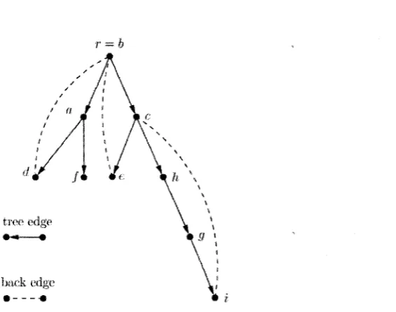
2.4 shows a depth-first tree of the graph shown in Figure 2.3.

A lgorithm 1 Depth First search

In p u t: the adjacency lists A of a connected graph G — (V, E).

O u tp u t: A depth-first search tree of G with vertices being assigned their DFS number

(the ranks of the vertices in the order they are visited by the depth-first search). In itia liz a tio n : count <— 1; r «— v, (u is arbitrary}

call D F S ( r);

R o u tin e D F S ( v);

make v as ’’visited” ; dfs(v) «— count; count *— count + 1;

fo r all vertex w in the adjacency list of v do if w is not visited th e n

call D F S ( w); e n d if

e n d for

e

h

a

J

d e h

a

h:

root

/

Figure 2.4: A depth-first search tree. The search starts at the vertex b, an arrow denotes a tree edge leading from parent to child; a dash line denotes a back-edge.

2.1.3

Tarjan’s Sequential B ico n n ectiv ity A lgorithm

Tarjan [39] presented a linear-time sequential algorithm for determining biconnected com­ ponents based on cut-vertices. The algorithm defines and computes the LOWPOINT values to detect cut-vertices, which has become a crucial technique for solving the bicon- necitivty problem. We give the following definition used in this algorithm for an arbitraxy vertex w of a given graph G = (V, E).

D efin itio n 2.1.14 \fw € V,

• low(w) = min({d/s(u;)} U {d/s(u)|{s, u} G B, for some descendants of w} ) , called the LO W PO IN T value of vertex w. [39]

• dfs(w): called the DFS number of vertex w, which is the rank o fw in the ordering the vertices are visited by the depth-first search.

• B: the set of all back-edges.

• C(w): the set of all children of vertex w.

L e m m a 2.1.2 low(w) = min({d/s(w)} U {low(w/)\w' is a child of w}U

{dfs(u)\(w,u)is a back-edge}),Vw G V.

P ro o f: See [39]. □

Proof: See [39]. □

Figure 2.5 shows a depth-first search tree of the graph given in Figure 2.3. Using Tarjan’s algorithm, the cut-vertices are identified to be a, b and c. The biconnected com­ ponents are subgraphs induced by the vertex sets {a, /} , {a, d, b}, {c, h, g, i} and {c, b, e}. Note that the intersection of each biconnected component and the D F S tree is a subtree of the D F S tree whose root is a cut-vertex.

r = b

back edge

A n O verview o f T a rja n ’s se q u e n tia l alg o rith m :

A lg o rith m 2 Tarjan’s Sequential Biconnected-Component Algorithm

1: In p u t: The adjacency lists of an undirected graph G = (V, E).

2: O u tp u t: The biconnected components of G.

3: Idea: Build a depth-first search tree T of G and compute the LO W PO IN T value of each vertex; when a cut-vertex is found, ou tp ut the subtree of T rooted at th a t cut-vertex.

4: In itia liz a tio n : count <— 1; r <— v; {v is arbitrary} 5: T <— 0; {T stores the edges of the D F S tree} 6: c a R D F S ( r , ± ) ;

7:

R o u tin e D F S ( v , u);

8: make v as “visited” ; dfs(v) <— count; count <— count + 1; loW(v) <— dfs{v); 9: for all vertex w in th e adjacency list of v do

10: if edge (v, w) has not been added to T th e n

11: T <- T U { 0 ,w )} ; 12: en d if

13: if w is not visited th e n

14: call DFS( w, v);

15: if (low[w) > df s(v)) th e n

16: T ' U {(v,?i,')} form the spanning tree of a biconnected component, where T ' is the subtree of T rooted a t w;

17: O utput and delete T ' U {(w, w)} from T; 18: e lse

19: low(v) <— mm{low(vy,low(w)}; 20: en d if

21: else

2 2: if (w u) th e n

23: low(v)<— min{/ow(^);dfs(w)}; 24: en d if

2.1.4

T h e P R A M B icon n ected C om ponent A lgorith m

Since all of the existing EM biconnected component algorithms simulate the correspond­ ing PRAM algorithm, we shall give a brief description of the PRAM algorithm, which is due to Tarjan and Vishkin [23, 40]. The algorithm is designed for the CRCW (concurrent- read-concurrent-write) PRAM model and takes 0(log(|V j)) time using 0{\V \ + |E |) pro­ cessors. Before discussing the PRAM algorithm,we shall give some definitions related to the algorithm.

D e fin itio n 2.1.15 E u le ria n G ra p h . A graph G = (V, E) is an Eulerian graph if it contains a circuit that traverses every edge of G exactly once. The circuit is an E u ler c irc u it or E u ler to u r of G.

D e fin itio n 2.1.16 T ra n sitiv e C lo su re. The tr a n s itiv e closure of a directed graph G = (V, E) is the graph G* = (V, E*), where E* consists of all ordered pairs < i , j > such that either i = j or there exists a directed path from i to j.

D e fin itio n 2.1.17 P r e o r d e r N u m b e r. The p reo rd e r tra v e rsa l of a tree T rooted at r is a sequence of vertices starting with the root r, following by the preorder traversals of the subtrees of r from left to right. The p reo rd e r num ber, pre(v), of vertex v is the rank of v in the preorder traversal o f T .

Given an undirected connected graph G = (V, E) and a spanning tree T of G, each nontree edge determines a fu n d a m e n ta l cycle which consists of the edge and the path in

T connecting the two end-points of the edge. Let R c be a relation in the set E defined by

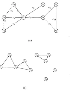
eRcg if and only if e and g belong to a common fundamental cycle. Then the tr a n s itiv e closu re o f R c, denoted by R*. partitions the edge set E of G into a collection of edge sets each of which induces a biconnected component of G. Therefore, the biconnected components of G can be determined as follows. Let G' = (V', E r), where V 1 = E and (e, g) G E ' if and only if eR cg. Then the connected components of G1 correspond to the equivalence classes of R* which uniquely identify the biconnected components of G. The graph G' of the relation R c is depicted in Figure 2.6. In (a), The set of fundamental cycles consists of C\ = e\, e3, e^, C2 = e2, e4, e5 and C-j = eg, eg, eio- The graph G' of the

relation R c is shown in (b). For example, there is an edge between e4 and e2 because

both e2 and e4 belong to the fundamental cycle C2. The connected components of G' are

{ei, e2, e3, e4, e5}, {e8,e9,e i0}, {eg} and {e7}, which define the biconnected components

of G.

(a)

Figure 2.6: An illustration of the graph G' of the relation R c. Figure (a) presents a graph

is identified by its preorder number. For any two edges e and g, eR'cg if and only if one of the following conditions holds (the parent of a vertex u is denoted by p(u) and the root of T is denoted by r ) : [23]

1. e = (u,p(u)) and g = (u,v) £ G — T and v < u.

2. e = (u, p(u)) and g — (v,p(v)) and (u,v) € G — T such th at u and v are not related (having no ancestral relationship).

3. e = (u,p(u)), g = (v,p(v)) such th at p(u) = v , v ^ r, and some nontree edge of G

joins a descendant of u to a non-descendant of v.

The PRAM algorithm computes R!c instead of R c, and for each v € V. let low(v) denote the smallest vertex th at is either a descendant of v or adjacent to a descendant of v by a nontree edge. Similarly, highly) denotes the largest vertex th at is either a descendant of v or adjacent to a descendant of v by a nontree edge. The algorithm is described below.

A lg o rith m 3 The PRAM Biconnected Component Algorithm

1: In p u t: A connected undirected graph G.

2: O u tp u t: An array C such that C(e) = C(g) if and only if e and g are in the same

biconnected component.

3: Construct a spanning tree T (not necessarily a D F S tree) of the input graph G.

4: Root T at an arbitrary vertex, and apply the Euler-tour technique to assign to each vertex its preorder number.

5: For each vertex v, compute two values low(v) and high(v).

6: Test conditions of R!c using the low. high values and build the auxiliary graph G '.

7: Find the connected components of Q . These connected components give rise to the biconnected components of G and are identified by an array C.

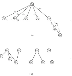
Figure 2.7: (a) A spanning tree represented by solid lines and the dashed edges are nontree edges, (b) The connected components of G' correspond to the biconnected components of G (a). The relation R'c defined by the three conditions. Condition 1: (6 4, ei); (e5,e2);

2 .2

M o d e l o f C o m p u ta tio n

Since retrieving d ata from the external disks requires a substantial amount of access time, a block, instead of a datum, is transferred between the external disks and the main mem­ ory. To simulate the behavior of I/O operations, Aggarwal and Jeffrey [2] proposed a standard two-level I/O system with one logical disk.

The External memory model we shall use is the Parallel D isk M odel (P D M ) [46] (see Figure 2.8.)

C P T

D i - k 1 D i^ k i • • * D i< k

I"

Figure 2.8: External Memory Model [46]p. 113

In this model, the external memory consists of D disks each of which is associated with a read/w rite head. During each I / O operation, the D disks can simultaneously transfer a block of B contiguous data items. Therefore, the total number of data items transferred in each I/O is D B. The following parameters are associated with the PDM:

• N = input size (in units of data items),

• M = internal memory size (in units of data items),

• B = block transfer size (in units of data items),

The lengths of the data items are all bounded by the same constant. The input data are stored in the external memory because they are too large to fit into the main mem­ ory. In general, M < N and 1 < D B < ^ • However, for graph-theoretic problems, let G = (V , E ) be the input graph, it is possible th at \V\ < M < \E\. In which case, the model is called s e m i- e x te r n a l m e m o r y m o d e l or s e m i- e x te r n a l m o d e l for short.

Since data items are transferred in blocks of B data items, it is therefore convenient to use the following parameters:

The input data are initially striped across the D disks in units of blocks. Specifically, the first block of B data items are stored on the first disk, the second block of B data items are stored on the second disk, . . . , the Dth. block of B data items are stored on the D th disk, the (D + l)th block of B data items are stored on the first disk, the (D + 2)th block of B data items are stored on the second disk, and so on. In this way, an input of

N data items can be read or written with 0 ( N / D B ) — O in jD ) I/Os.

The performance measure is expressed in terms of I / O com plexity. The I/O com­ plexity of an EM algorithm is the total number of I/O operations it performs.

Sorting and scanning a sequence of consecutive data items are two primitive opera­ tions that are frequently used in external-memory algorithms. The I/O complexity for scanning N consecutive data items striped across the disks is:

scan(IV) = ^

The I/O complexity for sorting N consecutive data items striped across the disks is:

Chapter 3

R eview o f th e Current State o f th e

A rt

In this chapter, we review works related to EM graph algorithms done in the last decade. We shall call the sequential algorithms, which were described in the previous chapter,

internal algorithms as opposed to external algorithms.

The first publication on EM graph algorithms was due to Ullman and Yannakakis [44], in which an external-memory transitive closure algorithm on a directed graph was pre­ sented. The algorithm is based on depth-first search traversal and topological sort. It requires 0(dfs(\V \, |£?|) + scan(\V\2 ^ \ E \ / M ) ) I/O s, where 0(dfs(\V \, l-EI) is the number of I/O s performed by the depth-first search algorithm. For the semi-external model (i.e.

V < M < E), Ullman and Yannakakis proposed an EM depth-first search algorithm th at performs 0(scan(|.E|) + |V|) I/O operations.

Chiang et al. [13] presented a number of EM graph algorithms. The algorithms rely heavily on external sorting. As a result, The asymptotic I/O bounds of their algorithms include the parameter sort(x) as a factor.

Abello et al. [1] developed a functional approach for solving graph problems on the external-memory model. They also showed th at on the semi-external model, their ap­ proach could solve the connected component problem in 0(scan(|.E|) logM/ B C(G)) I/O operations, where C(G) is the number of connected components in G.

op-timal EM breadth-first search. Subsequently, an EM breadth-first search algorithm for undirected graphs with bounded degree was presented by Meyer [32]. Later, Kumar and Schwabe [29] designed the EM binary heap data structure and tournament trees; as part of the result, they presented improved graph algorithms with amortized performance, for constructing a minimum spanning tree, breadth-first search and depth-first search, and single-source shortest paths.

Munagala and Ranade [34] presented improved techniques for solving the connectiv­ ity problem and undirected BFS problem. Arge [5] extended the technique to compute minimum spanning forest. In Chapter 1, we mentioned EM algorithms for solving the biconnectivity problem. These algorithms are not depth-first search based and hence do not use EM depth-first search although a large number of 1/O-efRcient depth-first search algorithms had been developed.

Chiang et al. [13] made a major contribution to the field by showing th at parallel algorithms for the PRAM can be simulated in the external model. Specifically, In each step of the simulation, input data are sorted and divided into independent sets by the indices of the processors on which they are required for computations of this step. These data sets are then read into the main memory by a scan operation. After each simulation step, the results are written back to the disks. The results are sorted again for the next simulation step. Each simulation step needs 0(sort(AT)) I/Os. Therefore, if a PRAM al­ gorithm runs in time T with N processors, the simulation will require 0 (T -so rt (AT)) I/Os.

3.1

T h e E x is tin g E M G r a p h -C o n n e c tiv ity A lg o r ith m

3.1.1 A D escrip tion o f th e A lgorith m

Chiang et al. [13] adapted the parallel connected component algorithm of Chin et al [14] to construct an EM connected component algorithm (or GCC). The input graph G — (V, E )

is represented by the adjacency lists of the vertices stored in a 2-dimensional array. The adjacency lists are stored on the external disks.

Each vertex belongs to exactly one connected component. The array D identifies, for each vertex, the connected component containing th at vertex. Consequently, D{i) = D(j)

if and only if vertices i and j belong to the same connected component.

Let V = {1,2,3,..., |Vj}. Chiang et al. use a 0(1) number of sorts to sort the edges of

G and a list ranking method to reduce the number of vertices during the following vertex reduction step:

A lgorithm 4 The EM_GCC algorithm of Chiang et al.

1: Initialization: Vi G V, D(i) <— i;

2: repeat

3: Vi G V, C(i) <- min{ j \j € Adj[i]}; 4: for all i G V do

5: if C(i) = N U L L th en

6: C(i) = i

7: end if

8: end for

9: Label each vertex i w ith “isolated”if and only if C(i) = i; {vertex i is isolated}

10: Vi G V, do D(i) «- C(i);

11: Apply th e list ranking algorithm to do Vi G V, C(i) <— C(C(i))\

12: Vi G V, D (i) = min{C'(i), D(C(i))};

13: Vi G V, do D{i) <- £>((£>(*));

14: Replace each edge (i, j ) in E by an edge (D(i), D (j)), where D(k) is th e super-vertex of th e connected component vertex to which k belongs;

15: Remove parallel edges and self-loops and vertices labelled w ith “isolated” 16: until |V| < M

E x p la n a tio n :

D: An array of length |V|. D(i) specifies the super-vertex into which vertex i is merged.

C: An array of length |V|. C(i) specifies the smallest-numbered vertex to which vertex i is adjacent.

On Line 1: Every vertex is a super-vertex initially. This step takes scan(|Vj) I/Os. On Line 3: For every vertex i, the smallest-numbered vertex among all the adjacent vertices is selected and assigned to C(i). In doing so, the adjacency list of i, Adj[i], has to be read into the main memory. Chiang et al. showed th at this step can be done with 0 (so rt(E )) I/Os.

On Lines 4-9: The isolated vertices are eliminated. Each of these isolated vertices is a super-vertex corresponding to a connected component of G.

On Lines 10-13: P ath compression is performed to merge the vertices into super­ vertices based on the list-ranking technique. Chiang et al. [13] presented a list ranking algorithm which runs on a jV-node link list in 0(sort(vV)) I/Os.

On Lines 14-15: The merged vertices are removed after all information about their adjacent vertices are transferred to the super-vertices. As a result, the size of the graph

G is reduced before the next iteration begins. This step requires a constant number of

The total number of I/O s performed in each iteration is sort (| £71). During each itera­ tion, a vertex reduction step is applied to reduce the number of vertices of G to at most

\V /M ] vertices. When the number of remaining vertices is less than or equal to M during the above reduction step, the reduced graph can fit into the main memory and the prob­ lem can be solved by the internal GCC algorithm. Therefore, log(|~V/M]) iterations are sufficient. Chiang et al. showed that Algorithm EM_GCC performs 0(log(V /M ) sort(E))

I/O operations.

3 .2

T h e E x is tin g E M B ic o n n e c tiv ity A lg o r ith m

3.2.1 A D escrip tion o f th e A lgorith m

As was mentioned in Chapter 2, the existing EM Biconnectivity algorithm (or EM_BCC) simulates the PRAM algorithm of Tarjan and Vishkin. Recall th at in explaining the PRAM BCC algorithm in Chapter 2, we mentioned th at the central idea of the EM BCC algorithm is to transform a given graph G into a graph G' such th at the connected com­ ponents of G' correspond to the biconnected components of G. Each vertex of G' is an edge of G. The edge (el, e2) exists in G' if and only if e l and e2 belong to the same cycle in G (Section 2.1.4).

A lgorithm 5 The EM_BCC Algorithm of Chiang et al.

1: Run Algorithm E M G en era te _ S p a n n in g T ree on a connected graph G — (V , E)

to construct an arbitrary spanning tree of G, denoted as T = (V , E t)• Algorithm Generate_SpanningTree is a slight modification of Algorithm EM_GCC.

2: Find an Eulerian circuit of T' = (V, E r). where T' is produced from T by duplicating every edge of th e latter.

3: Use Routine R o o t-T re e to convert T' into a rooted tree, T(r), w ith vertex r (r is arbitrary) being the root.

4: Run Routine E M E v alu ate_ T ree on the tree T (r) to com pute low(i) and high(i), for each vertex i.

5: Test the conditions of R'cusing th e values low(i) and high(i) to label the edges of T. Then, construct an auxiliary graph G'.

6: Apply A lgorithm E M _G C C to G' to determ ine its connected components.

E x p lan a tio n :

On Line 1: In Algorithm EM_GCC, the C(i) pointers induce a collection of trees. When the super-vertices are merged into larger super-vertices, the trees are also merged into larger trees. When execution of Algorithm EM.GCC terminates, the collection of trees are also merged into a spanning tree of G.

On Line 2: Let the spanning tree T of G generated on Line 1 be represented by the adjacency lists AdjT. An Eulerian circuit of T' — (V, E') can be determined by computing the su c ce sso r function s. Specifically, let Adjriv) = < u0, u-j,..., u<i-i >, where d is the degree of vertex v. The successor function s is defined as: s(< u-i, v >) ~ <

G ^(i+l) mod d -A 0 S: f d 1.

On Line 3: A rooted tree T ( r) with root r is constructed by applying the Euler-tour technique on T'. Routine Rooted-Tree (presented below) determines the parent of each vertex r) in T (r).

On Line 4, In the rooted tree T(r), each vertex is identified by its preorder number defined in Chapter 2. Routine EM Eavluate_Tree is presented below.

On Line 5: A list L of edges is created to determine the graph G' as follows [23]: By condition 1 of R'c, for each edge g = (u,v) E G — T such th at v < u, put the pair (e, g) in L, where e = (u,p(u)).

By condition 2 of R'c, for each edge (u,v) E G — T such that v + size(v) < u (size(v)

is the number of vertices in the subtree rooted at v), put the pair (e, g) in L, where

e = (u,p(u)) and g = (v,p(v)).

By condition 3 of R'c, for each edge e = (u,p(u)),p(u) = v ,v ^ r, put the pair (e, g)

into L if low(u) < v or high(u) > v + size(v), where g = (v,p(v)).

A lgorithm 6 Routine Rooted-Tree

1: Let r be an arbitrary vertex (the root);

2: s(< u, r > ) 4— 0, where vertex u is the last vertex of A d jrir);

3: Assign a weight of 1 to each arc < u, v >;

4: Apply the EM list ranking algorithm on the list defined by s; 5: if V < u, v >, (rank(< u, v >)) < (rank(< v, u >)) th e n

6: u = parent(v) 7: else

8: v = parent(u)

9: en d if

Explanation:

On Line 4: The list L defined by .s is a collection of arcs < r, u\ >, < Ui, u2

u\v\,r > such th at each arc < u,;, ui+1 >, 1 < i < |V|, except of the last one (the tail),

stores a pointer next to its successor in L. The list ranking problem is to compute the distance from the head (the first element) of L to each arc < Ui,Ui+\ >, denoted by

rank(< Ui,ui+1 >).

A lgorithm 7 EM Evaluate_Tree

1: {Compute the preorder number of each vertex v }

2: W (^ r) € V,

assign the weight w(< parent(v),v >) = 1 and w(< v,parent(v) >) = 0; 3: Apply the EM list ranking algorithm on the list defined by s;

4: Vu t£ r,E V, pre{u) <— rank(< parent{u),u >); pre{r) <— 0;

5: {Compute the low values of each vertex}

6: Vu € V, w(v) «— min({u} U {u\(v,u) is a nontree edge}) 7: Vu € V, low(v) <— min{w;(u)|u is in the subtree rooted at u}; 8: {Compute the high values of each vertex}

9: Vu € V, w(v) <— max({u} U {u|(u,«)is a nontree edge}); 10: Vw € V, high(v) <— max{w(u)|u is in the subtree rooted at u}

T h e o re m 3.2.1 Given a graph G = (V,E), the connected components, biconnected com­ ponents of G can be computed with min{log(V/M )(scan(E)),sort(V2)} I/Os.

P ro o f: See [13]. □

3 .3

A n E x is tin g E M D e p th -fir st Search A lg o r ith m

In [13], Chiang et al. presented an EM depth-first search algorithm for directed graph, henceforth called EM_DFS, th at requires 0((1 + V /M ) scan(E) + U) I/Os. Unfortunately, as the description, the correctness proof, and the time complexity analysis of the algo­ rithm they give are extremely terse, we shall first provide a detailed description of the algorithm in this chapter.

Since our objective is to develop I/O efficient algorithms for undirected graphs, we shall thus present our detailed explanation of Algorithm EM DFS in the context of undirected graphs. Note that every undirected graph can be viewed as a directed graph satisfying the condition: “there is a directed edge from vertex i to vertex j if and only if there is a directed edge from vertex j to vertex

L e m m a 3.3.1 The EM^DFS algorithm of Chiang et.al. can be executed on an undirected graph.

P ro o f: Immediate from the aforementioned condition. □

3.3.1

A D eta iled D escrip tion o f th e A lgorithm

The algorithm of Chiang et al. takes three arrays th at are stored on external disks as input. The arrays represent the input graph G = (V,E). One array A with a size of |i£| consists of the adjacency lists of the graph. The other two arrays, start and stop,

each with size |U| mark the beginning and the end, respectively, of the adjacency list of each vertex in array A. Specifically, for each vertex i, { A [)] ISf a rt [i] < j < Stop{i}\

consists of all the vertices adjacent to vertex i in G. W ithout loss of generality, we assume

V = {1,2,3,..., |U|}

To execute EM_DFS, the main memory is divided into two parts. One part is the input buffer consisting of a block of D B data units. It is used to transfer data between the external memory and the main memory. The other part is used to maintain an internal search structure and to maintain or keep data for booking purposes. For instance, the offset variables for calculating the location of the block of D B data units to be read into the main memory are kept in this part.

the current vertex of the search with an already visited vertex is being explored.

The algorithm maintains a stack in the external memory, called the DFS stack, to store the vertices on the path th at connects the root with the current vertex of the search. Ini­ tially, the stack is empty. Suppose the depth-first search starts at a vertex, say r. Then vertex r becomes the current vertex of the search. It is then inserted into the internal search structure. A section (a block of D B vertices) of the adjacency list of vertex r starting with A[start[r}\ is then read into the input buffer inside the main memory. Let A[start[r]] = v. The internal search structure is then searched for v. Since v is clearly unvisited, it cannot be in the search structure. Vertex v therefore becomes the current vertex. So, start[r) is updated to start[r\ + 1 and vertex r is pushed onto the DFS stack.

Note th at the updated start[r] points at the next vertex in the adjacency list of r to be examined when the search backtracks to vertex r in a later stage. Vertex v is then inserted into the internal search structure. The vertex is then processed in a way same as th at for vertex r described above.

In general, let vertex v be the current vertex of the depth-first search and a section of the adjacency list of vertex v starting from A[start[v]] has just been read into the main memory. Let A [start [u]] = u. The internal search structure is then searched for the vertex

u. If u is found in the search structure, then it is a visited vertex. So, the next vertex,

A[start[v] + 1], in the adjacency list is examined. If the vertex is again found in the search structure, then the next vertex in the adjacency list is examined. This is repeated until either an unvisited vertex, u, in the adjacency list is found or the section of adjacency list of v kept in the input buffer is completely examined. In the former case, the vertex u will become the current vertex. So start[v] is updated so that A[start[v\ — 1] = u, and vertex

v is pushed onto the DFS stack while vertex u is inserted into the search structure. In the latter case, the next section of the adjacency list of vertex v is read into the input buffer and the aforementioned process is repeated. If there is no next section of the adjacency list of v th at has not been examined, then the depth-first search must backtrack to the parent vertex of vertex v which is the top element on the DFS stack. Therefore, the stack is popped and the element popped out becomes the current vertex of the depth-first search.

These vertices represent edges th a t connect vertex v w ith visited vertices. Since these

edges will be ignored when they are being examined in a latter stage of th e search, they

can thus be discarded at this point of time. The array A is then com pacted so th a t all

the (unvisited) vertices rem ain in the list appear in a block of consecutive locations in the

external memory starting from the location ^4[1]. Furtherm ore, all the vertices belonging

to the same adjacency list are stored in a block of consecutive locations whose beginning

and end entries are marked by the updated start and stop pointers. After the array A

is cleaned up, the internal search structure is then em ptied and the depth-first search re­

sumes. Note th a t overflow can happen at th e internal search structure at most |"|K|/M ]

times. This is because every vertex can be inserted into the internal search structure

at most once and the internal search structure can accommodate O(M ) vertices. The

internal search structu re is needed until the array A is reduced to such a size th a t it could

fit into th e main memory.

The following is a formal description of Algorithm EM_DFS.

A lg o rith m 8 A lg o rith m EM-DFS of Chiang et al._________________________________ 1: Input: The arrays A[1 :: IE1)], start[1 :: \V\] and stop[1 :: |V|] representing a graph

g = iv, e).

2: O utput: A depth-first search spanning tree of the graph G. 3: Initialization:

4: S «— 0 ; {S' is the DFS stack}

5: P ush(£, 1); { vertex 1 is th e root of the DFS spanning tree } 6: InterS truct <— 0; { InterS truct is the internal search structure} 7: Store(InterStruct, 1);

8: w h ile not em pty (S) do

9: % <— Pop(S); { i is th e current vertex } 10: read (start[i\\stop[i\)\

11: w h ile (start[i] < stop[i]) do

12: w <— A[start[i]j; { get next vertex ready }

13: start[i] <— start[i] + 1; { update the start[i] pointer in the m ain memory} 14: if (w InterStruct) th e n

15: call Routine Unvisited-vertex; 16: en d if

A lgorithm 9 R outine Unvisited-vertex: To make an unvisited vertex the current vertex 1: (Insert w into the internal search structure}

2: if (InterS truct is full) th e n

3: call R o u tin e Compact-array to clean up;

4: e n d if

5: Store(InterStruct,w)] 6: vead(start[w],stop[m]);

7: read a block of A starting from A [start[w] ];

{w becomes the current vertex }

8; Push(5, i)\ w rite(sfart[i]); (update start[i}} 9: i w;

E x p lan a tio n :

On Lines 1 to 3, if an overflow occurs at the internal search structure, then the Routine Compact-array is called to clean up the internal search structure and to compact the array

A by removing all the visited vertices.

On Line 5, insert vertex w into the internal search structure to indicate th at it has become a visited vertex.

On Lines 6 and 7, a segment of the adjacency list of vertex w is read into the main memory.

On Line 8, the current vertex i is pushed onto the DFS stack and its start pointer is adjusted accordingly.

R o u tin e C o m p a c t-a rra y A: when InterStruct is full, for each vertex i, A[start[i]..stop[i}]

is scanned and all the visited vertices in it are deleted. The array A is compacted and the arrays start and stop are updated accordingly.

A lg o rith m 10 R o u tin e Compact-array A 1: for i fro m 1 to \V\ do

2: Determine the set B,t = {A[j]\(start[i\ < j < stop[i]) A (A[j] E InterStruct)}-, 3: Remove the vertices in R from A[start[i\..stop[i]\;

4: Compact the array A to make the remaining unvisited vertices consecutive;

5: Update start[i] and stop[i], accordingly; 6: e n d fo r

7: InterStruct <— 0.

E x p la n a tio n :

On Lines 2 and 3, the set of visited vertices in the current adjacency list of vertex i, Bi, is determined and the vertices are removed.

Lines 4 and 5 are self-explanatory.

On Line 7, the internal search structure is emptied.

3 .3.2

C orrectn ess P r o o f

When a vertex is examined for the first time during the depth-first search, we must mark the vertex as visited. To avoid using the expensive and slow I/O operation, we shall do the marking in the internal memory. The internal search structure is used for this purpose: whenever a vertex is first visited, it is inserted into the internal search structure. When it is encountered in a later stage, The internal search structured is searched and its presence in the structure indicates th at it is a visited vertex. Since a clean up is performed to the internal search structure whenever an overflow occurs, a visited vertex will no longer have an entry in the search structure after the clean up. As a result, when the vertex is encountered again in a later stage, it could be mistaken as an unvisited vertex as it does not appear in the internal search structure. Fortunately, owing to the fact the the array

A is also compacted whenever an overflow occurs at the search structure, once a vertex is removed from the search structure, it will never be examined again from another vertex.