Mining Image Dataset Using Decision Tree
Kajal Salekar
M.E Student, Dept. of I.T., Mumbai University, Pillai’s Institute of Information Technology, New Panvel, India
ABSTRACT: Mining Image dataset is one of the necessary features in the present development. The image datasets are used to store and retrieve the precious information from images, data mining on them. Pixel-wised image features were extracted and transformed into a database-like table which allows various data mining algorithms to make explorations on it. Each tuple of the transformed table has a feature descriptor formed by a set of features in combination with the target label of a particular pixel. With the label feature, we can accept the decision tree algorithm to understand relationships between attributes and the target label from image pixels, and to make a model for pixel-wised image processing according to a given training image dataset. The model can be very efficient and helpful for image processing and image mining.
It is likely that by using the model, various existing data mining and image processing methods could be worked on mutually in different behaviour. Our model can also be used to create new image processing methodologies, refine existing image processing methods, or act as a powerful image filter.
KEYWORDS: Image mining, Image mining Frameworks Mining techniques, Proposed model.
I. INTRODUCTION
Valuable information can be hidden in images, however, few research discuss data mining on them. In this paper, we propose a general framework based on the decision tree for mining and processing image data. Pixel-wised image features were extracted and transformed into a database-like table which allows various data mining algorithms to make explorations on it. Each tuple of the transformed table has a feature descriptor formed by a set of features in conjunction with the target label of a particular pixel. With the label feature, we can adopt the decision tree induction to realize relationships between attributes and the target label from image pixels, and to construct a model for pixel-wised image processing according to a given training image dataset. Both experimental and theoretical analyses were performed in this study. Their results show that the proposed model can be very efficient and effective for image processing and image mining.
II. RELATED WORK
Consider a general image mining and image processing framework and any existing decision tree algorithms can be used to do the job, we show only the testing result to simplify the expression. For the other results regarding the constructed classifier or the corresponding rules.
Step 1 -Image restoration with enhancement by using two types of synthetic images, numerals, english alphabet, with added noise artifacts.
Step 2 - The results shows that the noised images were successfully restored and enhanced. After we have settled the transformation details, a database-like table can be derived.
Step 3 - Applying a classification algorithm on the database-like table, a classifier for label prediction can be obtained. Step 4 - The ground truth from the experiments for image restoration with enhancement and image segmentation, respectively.
III.PROPOSED MODEL
classification is an essential part of many image segmentation methods, for example, determining pixels of an edge (corner) in edge (corner) detection methods, pixels of a particular object in objects segmentation based methods, pixels of abnormal tissue of medical image processing [1], and pixel classes in thresholding, etc. The model can be used to mine hidden relationships between an image’s pixel and its class label, and determine the interrelated features. Besides, the created model can be applied to perform pixel-wise segmentation on input images.
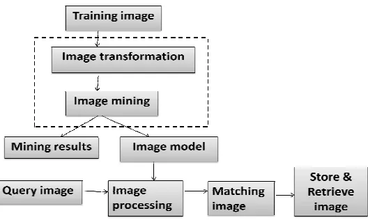
Figure 1. General processing flow of the Proposed System
These two phases are: image transformation and image mining.
Image Transformation Phase: This relates to how to transform input images into database-like tables and encode the related features.
Image Mining Phase: This relates to how to apply data mining algorithms on the transformed table and find useful information from it.
It is remarkable that the segmentation model is efficient, and requires only one scan of the date set. It can be used to effectively solve the time-consuming problem of segmentation with networks. Here we suggest two manners to apply our approach in similar situations.
The first one is using our model to substitute the existing method with the strategies mentioned above. The second one is using our model to quickly filter out the images that need advanced examinations. For example, after singling out suspicious mammograms that might contain pixels of cancer, one can apply the original method for second segmentation. The first manner is suitable for the case that our segmentation method result is better than the original one or the loss of correctness does not make significant difference. The second one is suitable for the case that the segmentation result is used in a critical manner, and the model is unable to reach that Requirement level. The model can easily extend from 2D to 3D image processing without making a revolution and the created model can generate very efficient and compact code.
A. Image Transformation and Feature Extraction
As mentioned, the input data of the proposed model is formatted as a set of equal sized raw and label image pairs. The transformation of the input image dataset into a database-like table and subsuming of the related features is described in this subsection. For the sake of clarity, various terms used for this process are defined below. In addition, we propose three kinds of input data sources.
Definition 2: The label image is a d-dimensional light-intensity function, denoted by L(c1, c2 to cd), where the value of L at spatial coordinates (c1, c2, to cd) gives the class identifier of the pixel at same spatial coordinates of its corresponding raw image.
Definition 3: The database-like table X = {x1, x2, to xt} is a set of records, where each record is a vector with elements <a1, a2, to ak> being the value of attributes (or features) of X.
In this example figure 4.2 shows, the raw image contains the capital English letter I with certain degree of blur. Thus, the inside pixels of the letter are darker and the outside pixels are brighter. If a pixel in the label image has the value 1, the pixel in the same position of the raw image is a pixel of outside contour. It is assumed to be a pixel of interest (POI) in this case. In practice, the pixel value of the label image is not limited to the binary form but could take any kind of form. In addition, we have as many raw and label image pairs at the same time as required for the input.
a) Raw image b) Label image
Figure. 2 An example for the input dataset.
In order to mine useful information from a set of raw and label images, we propose a methodology to transform them into a database-like table and allow any data mining algorithms to work on top of the table. This process is simple and straightforward the results of this transformation process according to the data in Figure. 4.3. Each row of such result table stands for a pixel its cardinality (number of rows) equals.
feature1 feature2 ..… featuren label
pixel1 7 2 …. value1n 1
pixel2 9 1.25 ….. value2n 0
pixel3 9 0 ….. value3n 0
….. …… ….. ….. …… ……
Pixeln 7 2 …… value25n 1
Figure.3 Result table of image transformation according to the input
In Figure 3, feature1 represents the gray level and feature2 the local variation. In order to simplify this demonstration, the local variation in this case is replaced with the average difference of a pixel to its 4-neighbors. Other pixel-wised features such as entropy, contrast, mean, etc. can also be encoded into the table as long as they might have affection on the collected dataset.
Various encoding strategies such as normalization (e.g., adjusting the value ranging from 0 to 1) or generalization (e.g., transforming the value to high, medium, or low) can be applied when generating the desired features. Moreover, the label image was included as a column in that table. With the presence of the label feature, hidden relationships between these two kinds of images can be mined.
7 9 9 9 7
5 7 9 7 5
0 7 9 7 0
5 7 9 7 5
7 9 9 9 7
7 9 9 9 7
5 7 9 7 5
0 7 9 7 0
5 7 9 7 5
Image Restoration with Enhancement
Image restoration with enhancement by using two types of synthetic images, Numerals English alphabet, with added noise artifacts. The noise artifact was generated by using the filter, add_noise, with a parameter of uniform distribution and the amount of 100%.The results in Fig. show that the noised images were successfully restored and enhanced. After we have settled the transformation details, a database-like table can be derived. By applying a classification algorithm on the database-like table, a classifier for label prediction can be obtained. Under the same way, testing images can be transformed into a database-like table to predict the label attributes. These predicted labels can moreover be visualized in a natural form of the input data, i.e., image. As we are proposing a general image mining and image processing framework and any existing decision tree algorithms can be used to do the job, we show only the testing result to simplify the demonstration. For the other results regarding the constructed classifier or the corresponding rules.
IV.DATA REDUCTION
Because of the image characteristics, pixels from a neighbouring area will generate similar feature vectors in the transformation process. Under some circumstances, it will cause remarkable redundant information in the result table; for example, an image with a large portion of background. Here we present some basic types of redundancy and show how they can be eliminated while converting the input image set.
Definition 4: The feature scope of a pixel M with spatial coordinates (c1, c2) is an n × n pixel area with centre at M, from which all the desired features of M can be generated. Usually n is an odd number, and the sub-image within the feature scope, i.e., pixels within spatial coordinates, is called the root space of the pixel M, denoted as {RSM}.
Definition 5: Two root spaces {RSN}, {RSO} are rotation reachable if {RSN} = {RSO}R, where {.}R stands for a root space after rotating the angle once by 90 degree, 180 degree, or 270 degree.
Definition 6: Two root spaces {RSN}, {RSO} are mirror reachable if {RSN} = {RSO}F, where {.}F stands for a root space after flipping horizontally or vertically. Given two pixels P and Q at different spatial coordinates of an image I, they are said to be:
Equivalent redundant, if {RSP} is equal to {RSQ},
Rotation redundant, if {RSP} and {RSQ} are rotation reachable,
Mirror redundant, if {RSP} and {RSQ} are mirror reachable,
Conflict redundant, if {RSP} and {RSQ} satisfy any one of the first three conditions, but the label information of pixels P and Q is not equal to each other.
V. PSEUDO CODE
Algorithm: Image Transformation
Step 1: Generate two image table raw and label
Step 2: Calculate the feature generate, label generates, initial table and pixel . Step 3: Check the pixel scanning process.
insert into table value :=
feature_generated1(raw, pixel),
…,
feature_generatedn(raw, pixel), label_generated(label, pixel);
Step 4: Continue to scan on the next pixel. Step 5: go to step 3.
Step 6: End.
Algorithm: Redundancy Reduction
Step 1: calling function RR
Step 3: if {RSC} can be matched in restore {redundant pixel}
discard {RSC} for further record generation;
Step 4: if the label information of the two matched entries are not equal do {conflict redundant pixel}
update the corresponding information in restore;
retrieve or update previously generated record if necessary; Step 5: else
{non-redundant pixel}
record all characterized redundancies of {RSC} and the corresponding label information in restore
Algorithm: Tree-Building
Step 1: Make Tree (Training Data T) Partition (T);
Step 2: Partition (Data S)
if (all points in S are in the same class)) then return; Evaluate splits for each attribute A
Use best split found to partition S into S1 and S2;
Partition (S1);
Partition (S2);
VI.SIMULATION RESULTS
After having obtained such a database-like table in accordance to the desired input image dataset, mining algorithms can then be used on it. We have chosen the decision tree for this purpose. An advantage of the decision tree over other methodologies. For instance, if the gray level of a given pixel ranges between 180 and 240 and its entropy is greater than 0.5, then it is a pixel of interest, POI. This basic idea of simplicity and easy understand ability is also the main principle of our approach. The results of such a mining process may help us to better understand the image properties and relate to real world instances. The results can also be used to process new images of the same domain. Basically, the result of the proposed model is a decision-tree Classifier by using C 4.5. A result classifier can be further straightforwardly translated into a set of human readable if-then rules. For instance, from the three leaf nodes in Figure. 4, they can obtain the following three rules:
If the gray level of a given pixel is less than 8 and its local variation is less than 5, then it is a pixel of outside contour.
If the gray level of a given pixel is less than 8 and its local variation is greater than or equal to 5, then it is not a pixel of outside contour.
If the gray level of a given pixel is greater than or equal to 8, then it is not a pixel of outside contour.
Figure 4 A decision tree for the concept is_outside_contour, indicating whether or not a pixel is a pixel of outside contour. gray level?
local variation? no
no yes
≥8
< 8
These rules can provide useful information about the training image. Besides, in order to obtain a higher level of appearance and meet the different information granularity requirements, the rules can be post-processed by rule induction algorithms. More importantly, we used to process new images from the same domain. The practical image processing capabilities include image restoration, image enhancement, image segmentation, etc. Both experimental and theoretical analyses were performed in this study to examine the proposed model. The built classifier can also be used to select important features. Features used at higher tree levels for the splitting criteria show a higher significant influence on the pixel class. The selected features can reflect the characteristics of the label image and help design or refine other image processing algorithms.
Most decision-tree classifiers (e.g. CART, C4.5) perform classification in two phases: Tree Building and Tree Pruning. Tree Building an initial decision tree is grown in this phase by repeatedly partitioning the training data. The training set is split into two or more partitions using an attribute. This process is repeated recursively until all the examples in each partition belong to one class below algorithm shows an overview of the process.
Tree Building: There are two main operations during tree building: i) evaluation of splits for each attribute and the selection of the best split and ii) creation of partitions using the best split. Having determined the overall best split, partitions can be created by a simple application of the splitting criterion to the data. Thecomplexity lies in determining the best split for each attribute. The choice of the splitting criterion depends on the domain of the attribute being numeric or categorical (attributes with a finite discrete set of possible values). But let us first specify how alternative splits for an attribute are compared. Splitting Index A splitting index is used to evaluate the “goodness” of the alternative splits for an attribute. Several splitting indices have been proposed in the past. We use the gini index, originally proposed. If a data set T contains examples from n classes, gini is defined as
gini(T) = 1 - ∑ pj2 (1) where pj is the relative frequency of class j in T.
Splits for Numeric Attributes: A binary split of the form A ≤ k, where k is a real number, is used for numeric attributes.
The first step in evaluating splits for numeric attributes is to sort the training examples based on the values of the attribute being considered for splitting. Let k1,k2 . . . , kn, be the sorted values of a numeric attribute A. Since any value between ki and ki+1 will divide the set into the same two subsets, we need to examine only n - 1 possible splits. Typically, the midpoint of each interval ki - ki+1 is chosen as the split point. The cost of evaluating splits for a numeric attribute is dominated by the cost of sorting the values. Therefore, an important scalability issue is the reduction of sorting costs for numeric attributes.
Splits for Character Attributes: If S(A) is the set of possible values of a character attribute A, then the split test is of the form A € S’, where S’ ∩ S. Since the number of possible subsets for an attribute with n possible values is 2n the search for the best subset can be expensive. Therefore, a fast algorithm for subset selection for a character attribute is essential.
VII. CONCLUSION AND FUTURE WORK
REFERENCES
1. Kun-che Lu And Don-lin Yang “Image Processing And Image Mining Using Decision Trees” Journal Of Information Science And Engineering 25, 989-1003, 2009.
2. J. Zhang, W. Hsu, and M. L. Lee, “Image mining: Issues, frameworks and techniques,” in Proceedings of the 2nd International Workshop Multimedia Data Mining, pp. 13-20, 2001.
3. K. C. Lu, D. L. Yang, and M. C. Hung, “Decision trees based image data mining and its application on image segmentation,” in proceedings of International Conferenceon Chinese Language Computing, pp. 81-86, 2002.
4. K. C. Lu, Image Processing and Image Mining Using Decision Trees: Fusing Data Mining and Image Processing, a publication of master thesis by VDM Verlag, 2008.
5. J. P. Eakins and M. E. Graham. Content-based image retrieval: a report to the JISC technology applications program. Northumbria Image Data Research Institute, 2000.
BIOGRAPHY