Fast Wavefront Reconstruction for Interferometric Data using LabVIEW

Fast Wavefront Reconstruction for

Interferometric Data using LabVIEW

M.Mohamed Ismail

1

and M.Mohamed Sathik

2

Research Scholar, Dept. of Computer Science, Sadakathullah Appa College, Tirunelveli, Tamilnadu, India 1

Principal, Sadakathullah Appa College, Tirunelveli, Tamilnadu, India 2

ABSTRACT: This paper presents an optimized noise-reduction algorithm for noisy interferometric fringe pattern image. We simulated an interferometric fringe pattern image and incorporated different additive type of Gaussian noises. Due to inclusion of the noise in the interferogram, the image is disturbed and it is important to retrieve phase information from fringes for further process of wavefront error estimation for the adaptive optics applications. This paper reports the faster denoising algorithm of 2D Fourier transform approach with data parallelism using LabVIEW in an optimized way. To reduce the data from the interferogram, single dimensional and two dimensional Fourier Transform are used for comparison of which is fast and accurate.

KEYWORDS: Adaptive Optics, Shearing Interferometer, 2D Fourier Transform, data parallelism.

I. INTRODUCTION

In Astronomical Instrumentation, the medium is the Earth’s turbulent atmosphere, and the optical signal is the light emitted by the star or the body of interest. The atmospheric turbulence can be considered as a random process and can be estimated by means of variances and co-variances of local refractive index fluctuations [1]. The turbulence affects the image quality at the focal plane of the telescope. Thus, the perfectly plane wave from a star at infinity is aberrated before it enters the telescope. The distortion induced by the turbulent atmosphere on the incoming wavefront from the stars can thus be corrected which enables the telescope to reach the diffraction-limited image quality, thereby improving the resolution of the ground-based telescopes. The real time correcting system is called as Adaptive Optics (AO). The fundamental components of an adaptive optical (AO) system are a wavefront sensor to measure the distortions in the optical beam, a wavefront corrector to compensate these errors, and an estimation and control algorithm to derive the control signals from the distortion measurements.

The most commonly used wavefront sensors are the Shack-Hartmann [2, 3] curvature sensing [4] shearing interferometry [5, 6] and Pyramid wavefront sensor [7]. Among the wavefront sensors, the Shack-Hartmann (SH) sensor is the most commonly used technique for measurement of turbulence for various applications in atmospheric studies and adaptive optics. Shearing interferometry has the important advantages over other wavefront sensors, i.e. it has very high resolution. It requires no reference wavefront for the production of fringes other than the incident wavefront itself i.e. Self-referenced measurement and particularly insensitive to environmental vibrations.

measures the distortions across the telescope pupil of the incident beam. To estimate these errors in real time, a suitable algorithm has been developed in Lab VIEW platform. We simulated the interferogram without any distortion and with distortion using Gaussian noise. Also, a suitable data reduction procedure using Fourier technique of the interferogram has been worked out which is giving full information of the errors present in the wavefront within few milliseconds.

1.1 Related Works

First we adopted the algorithm [18], as it proceeds the interferometric image was read row-by-row pixels (one dimensional). From this 1D data, the high frequencies were fitted to the Fast Fourier Transform. It retains the frequency corresponding to maximum amplitude along with few frequencies on both sides and make rest of the amplitude zero for all other frequencies. The high frequency noise was removed keeping only the data signal. After taking the inverse Fourier Transform the noise was partially removed. In this method, the simulated interferometric image has been used for computing the wavefront error which is time consuming that is main drawback for the algorithm. In adaptive optics real-time wavefront correction timing must be within 20 milliseconds. But the existing method to denoise the interferometric image has taken about 2000 milliseconds for image size of for 512 X 512 and 1300 milliseconds for 256 X 256. So for proposed new algorithm these problems are considered and suitable modification has been adopted.

II. INTERFEROGRAM SIMULATIONS USING ZERNIKE POLYNOMIAL

Zernike polynomials are widely used for describing the classical aberrations of an optical system [14]. They have the advantage that the low order polynomials are related to the classical aberrations like, spherical aberration, coma and astigmatism. Fried [15] used these Zernike polynomials to describe the statistical strength of aberrations produced by the atmospheric turbulence. The PSI wavefront sensor measures the wavefront slope. The derivatives of the Zernike Polynomials can be written as a linear combination of Zernike polynomial [16]. Hence, the slope information from the wavefront sensor can be conveniently expressed as a function of the Zernike polynomials. The basic interferometric equation for Zernike and the gradient of the Zernike polynomial is represented by

∆𝑍

_𝑗

= 𝛾

_{𝑗 𝑗}

′

𝑍

_𝑗

′

𝑗

′

(2.1)

where γ_jj′ are the coefficients of the Zernike expansion of the derivative of the jth Zernike. The matrix γ is called

Zernike derivative matrix and it is given in Noll, 1976. And the wavefront slope is explicitly written as

∆𝑊 𝑥, 𝑦 = 𝑎

_𝑗

𝑠 𝛾

_𝑥

_𝑗𝑗

𝑍

_𝑗

𝑗

+ 𝑡 𝛾

_𝑦

_𝑗𝑗

𝑍

_𝑗

𝑗

𝑛

𝑗 =1

(2.2)

Figure 1: Simulated PSI interferograms using the Zernike coefficients with only defocus term while all other coefficients is zero

III. EFFECT OF GAUSSIAN NOISE ON INTERFEROGRAM

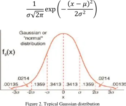
Gaussian noise is evenly distributed over the signal. This means that each pixel in the noisy image is the sum of the true pixel value and a random Gaussian distributed noise value. As the name indicates, this type of noise has a Gaussian distribution, which has a bell shaped probability distribution function given by equation

1

𝜎 2𝜋

exp −

𝑥 − 𝜇

2

2𝜎

2

(3.1)

Figure 2. Typical Gaussian distribution

Where x represents the gray level, μ is the mean or average of the function and σ is the standard deviation of the noise. Varying sigma we get the distorted interferometric image.

(a) (b)

(c) (d)

Figure 2. Noisy interferogram with Gaussian noise level of 0.3, 0.5, 1 and 1.5

IV. TIME REDUCTION WITH 2DFAST FOURIER TRANSFORM METHOD

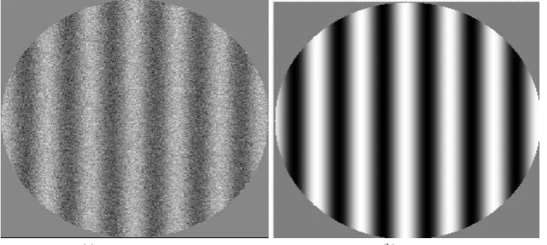
In this proposal we adopted the 2D FFT which is giving noise free image with reduced time. We opted for 2D FFT, which computes the discrete Fourier transform (DFT) of the input matrix. This FFT performs a 1D FFT on the rows of the input matrix and then performs a 1D FFT on the columns of the output in the preceding step. When FFT is the Fourier transform of a 2D real time-domain signal with M rows and N columns, the lower half part of FFT can be constructed by the upper half part. The figure 3 a, b shows that the noisy fringe affected by Gaussian noise and its denoised image using single Dimensional FFT. The figure 4 a, b shows that the noisy fringe affected by Gaussian noise and its denoised image using two dimensional FFT.

The DFT of an M-by-N matrix is defined as:

𝛾 𝑢, 𝑣 = 𝑥(𝑚, 𝑛)𝑒−𝑗 2𝜋𝑚 𝑢 𝑀 𝑁−1

𝑛=0 𝑀−1

𝑚 =0

𝑒−𝑗 2𝜋𝑚 𝑣 𝑛 _{𝑓𝑜𝑟 𝑢 = 0,1,2 … , 𝑀 − 1, 𝑣 = 0,1,2 … , 𝑁 − 1}

_(4.1)

Where x is the input matrix and γ is the transform result. The figure 3 shows that the noisy interferogram and denoised interferogram using 1D FFT method of existing algorithm [18].

(a) (b)

Figure 3. The noisy image (a) and denoised image using single dimensional FFT (b)

The figure 4 shows that the noisy interferogram and denoised interferogram using 2D FFT method of proposed algorithm.

V. RECONSTRUCTIONOFTHEDISTORTEDWAVEFRONT

The phase thus recovered is measured with an integral multiple of 2π uncertainties. The process of removing these uncertainties is called phase unwrapping. After phase has been completely unwrapped, the data contains the derivatives of the original phase of the wavefront. The derivative of the wavefront phase can conveniently be written in terms of Zernike polynomials, to estimate the wavefront errors. The Zernike coefficients provide the complete information of the wavefront.

A. Wavefront determination from wavefront slope data using Zernike polynomial

The aberrated wavefront has to be reconstructed from the wavefront slopes derived from the above method. The wavefront aberrations can be well represented by Zernike polynomials. The derivatives of the Zernike polynomials can be expressed as a linear combination of Zernike polynomial [16]. They are written as

∆𝑍𝑗 = 𝛾𝑗 𝑗′𝑍𝑗′ 𝑗′ (5.1) Alternatively ∆𝜑 = 𝑎𝑗𝛾𝑗 𝑗′ 𝑗 𝑍𝑗 𝑗

(5.2)

Where

𝛾

_{𝑗 𝑗}′are the coefficients of the Zernike expansion of the derivative of the jth Zernike. The matrix

γ

is called Zernike derivative matrix and it is given in [16]. The wavefront slope as derived from this method can be written as in equation 5.3. ∆𝑊(𝑥, 𝑦) =𝜕𝑊 𝜕𝑥 𝑠 + 𝜕𝑊 𝜕𝑦 𝑡 (5.3) 𝜕𝑊 𝜕𝑥 = 𝑎𝑗𝛾𝑗 𝑗′ 𝑥 𝑗 𝑍𝑗 𝑎𝑛𝑑 𝑗 𝜕𝑊 𝜕𝑦 = 𝑎𝑗𝛾𝑗 𝑗′ 𝑦 𝑗 𝑍𝑗 𝑗 (5.4) So that combining (5.2), (5.3) and (5.4),

∆𝑊(𝑥, 𝑦) = 𝑠 𝑎𝑗𝛾𝑗 𝑗′ 𝑥 𝑗 𝑍𝑗 𝑗 + 𝑡 𝑎𝑗𝛾_{𝑗 𝑗}𝑦′ 𝑗 𝑍𝑗 𝑗

(5.5)

In matrix notation this equation can be written as

W = A Z

W ZT = A ZZT

W ZT (ZZT)-1 = A (ZZT) (ZZT)-1 (5.6)

A = W ZT (ZZT)-1

A provides the Zernike coefficients. Using the Zernike coefficients, the aberrated wavefront is reconstructed as

𝑊(𝑥, 𝑦) = 𝑎𝑗 𝑁

𝑗 =2

𝑍𝑗

(5.7)

where ajare the Zernike expansion coefficients. So far the considerations have involved, derivations based on the

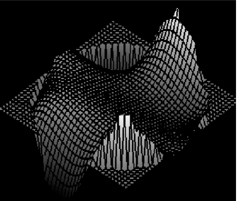
theory for ∆Wx and ∆Wy, with the resulting polynomial expressions formulated in terms of circle of unit radius. The Figure 5 shows that the 2D wavefront error map computed from noisy interferometric image fringe pattern.

Figure 5. The 2D wavefront error map as computed from the Zernike polynomials

VI. TIME REDUCTION WITH DATA PARALLELISM USING LABVIEW

Figure 6.Typical representation of Data Parallelism used in LabVIEW

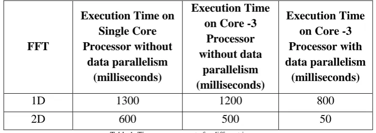
The following table shows the comparison of computing time for image size 256 X 256 using single dimensional FFT and 2D FFT. But the required time is 20 milliseconds. It is really achievable using multi core systems with parallel programming.

FFT

Execution Time on

Single Core

Processor without

data parallelism

(milliseconds)

Execution Time

on Core -3

Processor

without data

parallelism

(milliseconds)

Execution Time

on Core -3

Processor with

data parallelism

(milliseconds)

1D

1300

1200

800

2D

600

500

50

Table 1. Time measurements for different images

VII. CONCLUSION

In this paper, we attempted to simulate the fringe pattern with respect to shearing interferometer using Zernike polynomials. The wavefront errors are incorporated by adding Gaussian noise in the interferogram. We reported that the denoising method using 2D FFT using data parallelism in optimized way to reduce the time compare to the existing algorithm. We utilized the use of Fourier transforms techniques to estimate the wavefront errors in an optimized way using 2D FFT. In an adaptive optics situation, one requires a fast method of wavefront sensing and reconstruction. We included data parallelism for fast computation and the total was drastically reduced from 1300 milliseconds to 50 milliseconds.

REFERENCES

1. Hardy, J.W, “Adaptive Optics for Astronomical Telescopes”, 1998.

2. Platt, B. C. & Shack, R. V. (2001), “History and principles of Shack-Hartmann wavefront sensing”, Journal of Refractive Surgery, Vol. 17: S573–S577.

3. Shack, R. V. & Platt, B. C. (1971), “Production and use of a lenticular Hartmann screen”, J. Opt. Soc. Am., Vol. 61: 656. 4. Roddier, E. (1988), “Curvature sensing and compensation: a new concept in adaptive optics” , Appl. Opt., Vol. 27: 1223–1225.

5. Hardy, J.W. and Alan J. Mac Govern, “Shearing interferometry: a flexible technique for wavefront measurement” SPIE, Vol. 816, “Interferometric Metrology”, 180 – 195 (1987).

6. Atad E; John W. Harris; Colin M. Humphries; Victoria C. Salter, “Lateral Shearing interferometry: evaluation and control of the performance of astronomical telescopes” SPIE 1236, “Advanced Technology Optical Telescopes IV”, Lawrence D. Barr, Editors, 575-584 (1990)

7. Ragazzoni, R. & Farinato, J. (1999), “Phase retrieval and diversity in adaptive optics”, Opt. Eng., Vol. 350: L23–L26.

Dataset

CPU Core I

CPU Core II

8. J.W.Hardy, J.E.Lefebvre and C.L.Koliopoulous, “Real-time atmospheric compensation.” J.Opt.Soc.Am. 67, 360-369 (1977). 9. J.W.Hardy, “Adaptive Optics: a new technology for the control of light,” Proc.IEEE 66, 651-697 (1978).

10. A.K.Saxena, “Quantitative Test for concave aspheric surfaces using a Babinet Compensator,” Appl.Opt. 18, 2897 (1979)

11. A.K.Saxena and A.P.Jayarajan, “Testing concave aspheric surfaces: Use of two crossed Babinet Compensators”, Appl.Opt. 20, 724 (1980)

12. A.K.Saxena and J.P.Lancelot, “Theoretical fringe profiles with crossed Babinet compensators in testing concave aspheric surfaces,” Appl.Opt. 21, 4030-4032 (1982)

13. A.K.Saxena and J.P.Lancelot, “Wavefront sensing and evaluation using two crossed Babinet compensators,” SPIE, 1121, 41-43 (1990). 14. Born E and Wolf, “Principles of Optics” Pergamon Press. (1970).

15. Fried, D.L. “Statistics of a geometrical representation of wavefront distortion” J.Opt.Soc.Am, Vol.55, No.11, 1427 – 1435 (1965). 16. Noll, R.J., “Zernike polynomials and atmospheric turbulence” J. Opt. Soc. Am., Vol. 66, No.3, 207 – 211 (1976).

17. J.P.Lancelot, Ajay Kumar Saxena, “Extended Use of two crossed Babinet Compensators for Wavefront Sensing in Adaptive Optics”, SPIE, J.Adaptive optics,Vol-49,Issue – 12.