ABSTRACT
HYGH, JANELLE SUZANNE. Implementing Energy Simulation as a Design Tool in Conceptual Building Design with Regression Analysis. (Under the direction of Dr. Joseph DeCarolis.)
Whole building energy simulation is generally used to validate designs; however, its use as a decision support tool during design—especially during early stages—has been limited. Challenges with energy simulation implementation during conceptual design include the difficulty of creating an energy model with many unspecified parameters and the amount of time required to create an energy model and generate results. Use of a simplified simulation building program provides a practical alternative, but produces less accurate results due to the simplification of the complex processes governing the interaction of a building with its environment.
Implementing Energy Simulation as a Design Tool in Conceptual Building Design with Regression Analysis
by
Janelle Suzanne Hygh
A thesis submitted to the Graduate Faculty of North Carolina State University
in partial fulfillment of the requirements for the degree of
Master of Science
Civil Engineering
Raleigh, North Carolina
2011
APPROVED BY:
_______________________________ ______________________________
Dr. Ranji Ranjithan Prof. David B. Hill, AIA
DEDICATION
BIOGRAPHY
ACKNOWLEDGMENTS
I would first like to thank my committee for allowing me to be a part of this project. I have been able to study something I’m passionate about, and grown as a student, teacher, and researcher in the process. Ranji, Joe, and David – you have an uncommon dedication to your students and your professions. I hope I can continue that passion and dedication in my future endeavors.
I would also like to acknowledge the other people whose discussion and contributions have added to this work: Maria Papiez, Shawna Hammon, Dennis Stallings and colleagues at PBC+L.
To my father, thanks for your countless hours of Perl programming that made this project possible. Working with you has been a joy.
To my parents and family who have stood by me, supported me, and loved me during my best and worst times. I would not be here today if it weren’t for you.
TABLE OF CONTENTS
LIST OF TABLES ... vi
LIST OF FIGURES ... vii
Chapter 1 Introduction... 1
Chapter 2 Approach and Methodology... 4
2.1 Overall Approach ... 5
2.2 Methodology ... 6
2.2.1 Design Problem Set-Up... 6
2.2.2 Monte Carlo Simulation ... 7
2.2.3 Analysis ... 8
2.3 Intended Use... 9
Chapter 3 Illustrative Example... 10
3.1 Set-up ... 10
3.1.1 Design Parameters... 11
3.1.2 Simulation in EnergyPlus... 15
3.1.3 Data Processing ... 15
3.2 Regression Analysis ... 16
3.2.1 Refining the Regression ... 18
3.3 Parameter Sensitivity ... 25
3.3.1 EnergyPlus Results... 25
3.3.2 Parameter Sensitivity Methodology ... 27
3.3.3 Results ... 32
3.3.4 Validation ... 39
3.4 Number of Samples... 42
Chapter 4 Discussion... 44
4.1 Use as a Design Tool ... 44
4.2 Further Work... 46
4.3 Conclusion ... 46
LIST OF TABLES
Table 3.1: Annual cooling and heating degree-days for the TMY3 climate data... 10 Table 3.2: Description of Energy Model Inputs ... 11 Table 3.3: Design Parameters and Ranges of Sampling ... 12 Table 3.4: Equivalent cardinal direction for properties assigned to Sides 1-4 in energy model
input ... 16 Table 3.5: Variables added to heating regression model for Winston-Salem... 19 Table 3.6: Validation results for refined regression model using additional terms to capture
interactions between parameters and non-linear contributions of parameters... 20 Table 3.7: Regression coefficients from multivariate linear regression on heating load for
Minneapolis, MN ... 28 Table 3.8: Validation results for the multivariate linear regression on heating, cooling, and
total energy consumption... 39 Table 3.9: Average and standard deviation of percent error for heating, cooling, and total
LIST OF FIGURES
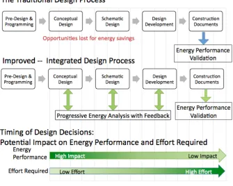
Figure 1.1: Traditional versus improved design process ... 1
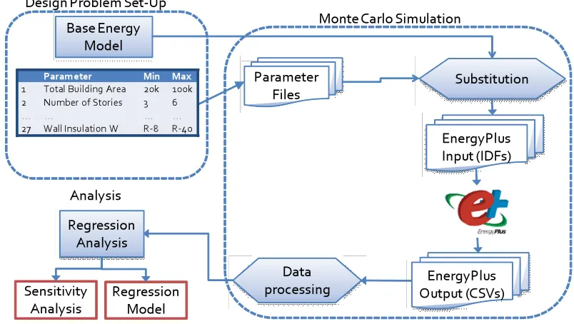
Figure 2.1: Framework for Monte Carlo simulation... 5
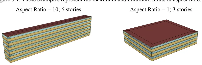
Figure 3.1: Example building geometries... 12
Figure 3.2: Rectangular building with relevant geometry parameters... 14
Figure 3.3: Diagram that describes the building orientation by cardinal direction. ... 16
Figure 3.4: Remaining RMSE as a function of the additional included parameters... 19
Figure 3.5: Root mean square error (RMSE) observed in heating, cooling, and total energy regression equations when compared to EnergyPlus results in the validation set... 22
Figure 3.6: Validation of the cooling regression model for the Albuquerque location. ... 23
Figure 3.7: Validation of the heating, cooling, and total energy regression models ... 24
Figure 3.8: Distribution of total heating and cooling energy for the four locations tested... 26
Figure 3.9: Cooling and heating energy results for the four locations tested ... 27
Figure 3.10: Parameter sensitivity based on the Miami regression model ... 29
Figure 3.11: Parameter sensitivity based on the Winston-Salem regression model ... 30
Figure 3.12: Parameter sensitivity based on the Albuquerque regression model ... 31
Figure 3.13: Parameter sensitivity based on the Minneapolis regression model... 32
Figure 3.14: Standardized regression coefficients for heating load at all four locations... 34
Figure 3.15: Standardized regression coefficients for cooling load at all four locations ... 35
Figure 3.16: Standardized regression coefficients for total energy consumption at all four locations ... 36
Figure 3.17: Comparison of raw linear regression coefficients showing sensitivity of building area and aspect ratio at all four locations... 37
Figure 3.18: Comparison of raw linear regression coefficients for window U-value and window-to-wall ratio at all four locations... 38
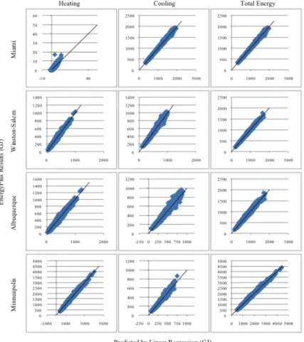
Figure 3.19: Validation of linear regression to predict energy consumption compared to EnergyPlus results... 41
Figure 3.20: Average prediction error of the validation set versus the number of estimation samples used to generate the multivariate regression ... 43
Chapter 1
Introduction
building design (Jacobs and Henderson 2002). These observations, although dated, still apply to current practice. Energy simulation is primarily used to estimate energy consumption to verify designs and demonstrate code compliance at the end of the design process (Lam et al. 2004; Morbitzer 2003; Rizos 2007). The incorporation of building energy analysis to support design is shown in Figure 1.1, which compares the current approach with an improved process that enables energy analysis to inform building design throughout the design process.
The high level of detail that is fundamental to energy simulation tools limits their use in the design process. Due to the complexity and detailed input required, performing energy simulation at early stages of design requires significant time, resources, and technical expertise. Contractual arrangements normally focus resources on the detailed design stage, thereby limiting the opportunities for energy analysis early in the process. The lack of smooth interoperability between design and analysis tools also limits the automatic exchange of building information, adding to the time requirements of creating an energy model and updating it as the design progresses.
The methods of analysis and communication of results should also be relevant to design decisions. Point estimates of energy consumption in conceptual design are not necessarily useful due to the uncertainty stemming from future design decisions that have not yet been made. Energy simulation in early design stages is useful, however, for comparative analysis, though this presents another challenge in requiring an energy model for each design alternative. Instead, if energy simulation tools facilitate broader search of the design space (e.g., by supporting parametric analysis of a whole building or a single room, floor, or façade in isolation), then the results could relate energy performance to key design parameters being explored. Such an approach would offer more meaningful insights and feedback to designers.
Chapter 2
Approach and Methodology
2.1 Overall Approach
The approach starts with a generic building of a specific type (e.g., medium size office building) with the simplicity and level of detail characteristic of a project in conceptual design, but complex enough to constitute a realistic design problem. Knowledge of energy performance with respect to key design parameters in conceptual design for the generic building can be generalized and made meaningful to many design projects. To eliminate the inputs normally required for a detailed simulation tool, assumptions for inputs defined later in the design process are selected to partially define the base energy model (see Figure 2.1). Identification of key parameters relevant to conceptual design decisions and the associated ranges of possible values define the design space explored in this approach. To sample the design space, Monte Carlo analysis is used to test combinations of parameters within their defined ranges. Monte Carlo simulation results serve as a rich data set, which is used to develop the regression model and validate it against independent EnergyPlus results. Sensitivity analysis using the simulation data also provides parameter sensitivities, or relative importance, of each to energy consumption.
2.2 Methodology
The approach in Figure 2.1 is realized through three main steps, each of which is described below.
2.2.1 Design Problem Set-Up
The first step starts with configuring the base energy model, which contains assumptions for all necessary energy simulation inputs intended to be implicit in the model developed in this work. Because the purpose of this approach is to develop a model that can be applied to similar projects, the base energy model must be sufficiently generic. Capozzoli et al. (2009) demonstrates this idea by focusing on a typical multi-storey office building, though they limited the analysis to a very simple intermediate floor. The base energy model must also be complex enough to constitute a realistic design problem to be relevant in the design process. Hopfe et al. (2007a), Struck and Hensen (2007), and Struck et al. (2009) apply uncertainty and sensitivity analysis to BESTEST cases, the benchmark energy models used to validate energy simulation programs, with simple geometry consisting of a single zone box with windows, but discuss the use of more realistic design problems. The base energy model with a set of assumed values serves as the starting point for the Monte Carlo simulation, which replaces the targeted parameter values with randomly chosen values distributed uniformly within a prescribed range. Two basic categories of information make up the building model: thermal information and geometry. Thermal information includes site location, monthly ground temperature values, internal loads and schedules, thermostat settings, construction assemblies and material properties, and other site-specific conditions. Geometry must be defined in the model and if it is not held constant, then it must be handled parametrically in the Monte Carlo analysis.
parameters. In this work, identification of key building parameters likely to affect building energy consumption during conceptual design were selected in consultation with David Hill, an architect on the research project and available literature (Krygiel and Nies 2008; Macdonald et al. 2005). After the parameters are chosen, continuous ranges or sets of discrete values for the parameters are assigned to be compatible with the options available in design.
2.2.2 Monte Carlo Simulation
Monte Carlo simulation explores the building energy performance space associated with the range of all identified parameters. An energy simulation tool calculates the energy performance for each sample in the Monte Carlo Simulation. EnergyPlus (Crawley et al. 1999) was chosen as the energy simulation tool in this methodology because it:
• Is the official energy analysis and thermal load simulation program of the U.S. Department of Energy
• Uses text input and output, which are easy to use in an automated workflow • Is based on first principles, not simplified algorithms
• Is freely available (non-proprietary) • Includes extensive documentation
• Allows for visualization and limited modification of an energy model using OpenStudio, a plug-in for Google SketchUp1
• Is available for Windows, Mac, and Linux
The Monte Carlo analysis starts by sampling each parameter and substituting the sampled values into the base energy model. To complete the substitution, the values of each parameter must be inserted in the appropriate location in the energy model. EnergyPlus does have built-in parametric objects that allow users to input values corresponding to multiple runs. Tags in the energy model correspond to parametric objects. When EnergyPlus finds that tag, it substitutes the value for that run as defined in the parametric object. While this is
useful for a limited number of parametric runs, it is quite cumbersome in a large Monte Carlo simulation. jEplus is another open source tool that enables large parametric runs using parameter trees with EnergyPlus and works with tags embedded in the EnergyPlus Input Data File (IDF) file (Zhang 2009). In this work, Perl scripts were utilized to make the substitutions in the IDF files. Instead of embedding tags, the Perl scripts use regular expressions to find EnergyPlus objects by name and type and make the appropriate substitution. This approach also makes the methodology easier to port between different energy models because it avoids the need to insert tags at every substitution location.
Though many runs of the energy simulation tool are required in the Monte Carlo analysis, a computationally expensive tool, EnergyPlus, is chosen in this framework. Lam et al. (2004) argue to avoid abstraction and rule-of-thumb approaches and use instead “first principle-based engineering algorithms” for accurate results, an approach aided by the increasing affordability of computing power. Using EnergyPlus avoids additional uncertainty introduced by simplifying algorithms, and because it is a highly configurable tool, it can be used for detailed design. This paper builds on the work described by other researchers, such as Capozzoli et al. (2009), who conducted sensitivity and regression analysis focusing on design variables with architectural significance, as the results were based on the quasi-steady simplified monthly method per ISO 13790: 2008. The importance of using detailed simulation tools is illustrated in a study using BESTEST case 600, a benchmark energy model used to validate energy simulation programs, that found significantly different uncertainties in output (e.g., up to 45% in annual cooling demand and 50% in peak cooling demand), among different simulation tools (Hopfe et al. 2007b). Inconsistent results among tools led Struck et al. (2009) to conclude that future research with sensitivity and uncertainty analysis should use sophisticated tools with simplified interfaces, not abstracted models with a corresponding interface.
2.2.3 Analysis
Validation with independent EnergyPlus results determines the efficacy of using the regression model in place of direct simulation, which is the ultimate goal of this work. This approach is similar in process to the building envelope trade-off option in ASHRAE 90.1-2007 (ASHRAE 90.1-2007): both perform regression on many energy simulations to obtain simple equations. This work differs, however, in its purpose to enable decision-making in conceptual design rather than demonstrate compliance of the final design of envelope components. Also, Capozzoli et al. (2009) perform regression on results that varied six heating and cooling variables, which yield adjusted R2 between 87.9% and 95.2%, and suggest that regression could be substituted for the quasi-steady simplified monthly method per ISO 13790. The work described in this paper represents a significant advancement over prior work by using a highly detailed simulation tool to develop a multivariate regression model based on 27 geometric and non-geometric design parameters. Sensitivities can also be extracted from the data produced by the Monte Carlo analysis to help architects target the most energy-sensitive design parameters during conceptual design.
2.3 Intended Use
This approach of developing a simplified regression model based on a large set of simulation results can provide meaningful feedback and insights to designers throughout the early stages of design. The goal is to develop a generic regression model that can be applied to a range of similar projects. The regression model can give approximate predictions of heating, cooling, or total heating and cooling building energy consumption for any set of key parameter values, with a margin of error calculated during regression model validation. Additionally, sensitivity analysis provides meaningful insight into the relative importance of different design parameters. The next chapter describes an illustrative study that demonstrates the development of this approach for an office building in four locations in the U.S.
Chapter 3
Illustrative Example
The methodology is presented for a rectangular, medium-sized office building, which is analyzed in four climate zones (ASHRAE 2007): 1A- Miami, FL, 4A- Winston Salem, NC2, 4B- Albuquerque, NM, and 6A- Minneapolis, MN. Table 3.1 provides a comparison of the climate in all locations described by annual cooling and annual heating degree-days with an 18°C baseline.
Table 3.1: Annual cooling and heating degree-days for the TMY3 climate data used for each location (Wilcox and Marion 2008)
Miami, FL (1A) Winston-Salem (4A) Albuquerque (4B) Minneapolis (6A) Annual cooling
degree-days 2442 724 724 454
Annual heating
degree-days 67 1695 2303 4202
3.1 Set-up
In this application, changes in form are governed by total building area, aspect ratio (the ratio of building length to depth), and number of stories. The base energy model for each climate zone is identical, except the ground temperatures and weather file used for the energy simulation. Details on the base energy model are provided in Table 3.2.
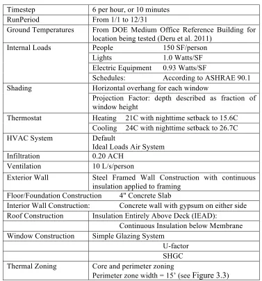
Table 3.2: Description of Energy Model Inputs
Timestep 6 per hour, or 10 minutes RunPeriod From 1/1 to 12/31
Ground Temperatures From DOE Medium Office Reference Building for location being tested (Deru et al. 2011)
Internal Loads People 150 SF/person Lights 1.0 Watts/SF Electric Equipment 0.93 Watts/SF
Schedules: According to ASHRAE 90.1 Shading Horizontal overhang for each window
Projection Factor: depth described as fraction of window height
Thermostat Heating 21C with nighttime setback to 15.6C Cooling 24C with nighttime setback to 26.7C HVAC System Default
Ideal Loads Air System Infiltration 0.20 ACH
Ventilation 10 L/s/person
Exterior Wall Steel Framed Wall Construction with continuous insulation applied to framing
Floor/Foundation Construction 4" Concrete Slab
Interior Wall Construction: Concrete wall with gypsum on either side Roof Construction Insulation Entirely Above Deck (IEAD):
Continuous Insulation below Membrane Window Construction Simple Glazing System
U-factor SHGC Thermal Zoning Core and perimeter zoning
Perimeter zone width = 15’ (see Figure 3.3)
3.1.1 Design Parameters
of stories, which can only take on integer values. Minimum and maximum values were chosen to allow for exploration of plausible design values; the ranges assigned for each parameter can be found in Table 3.3.
Table 3.3: Design Parameters and Ranges of Sampling
Parameter Unit Minimum Maximum
1 Total Building Area Area (SF) 20,000 100,000
2 Number of Stories - 3 6
Depth Ft 40 ft min; range governed by aspect ratio range
3
Aspect Ratio Length/Depth 1 10
4 Orientation (rotation) Degrees 0 180
5 Roof Insulation
R-value(h·ft2·°F/BTU)
15 50
6 Roof Color Solar Absorptance 0.19 0.97
7 Roof Emissivity Emissivity 0.86 0.95
8-11 Window R-value (N,S,E,W)
R-value (h·ft2·°F/BTU)
1.1 4.3
12-15 Window SHGC (N,S,E,W)
SHGC 0.2 0.6
16-19 Wall Insulation (N,S,E,W)
R-value (h·ft2·°F/BTU)
R-8 R-40
20-23 Shading Projection Factor (N,S,E,W)
Percentage of Window Height
5 100
24-27 Window to Wall Ratio (N,S,E,W)
% 2 90
Two examples of allowable building geometry in this sampling scheme are shown in Figure 3.1. These examples represent the maximum and minimum limits in aspect ratio.
Aspect Ratio = 10; 6 stories Aspect Ratio = 1; 3 stories
Window-to-wall ratio, window R-value, window solar heat gain coefficient (SHGC), wall insulation R-value, and shading projection factor were considered independently on each face of the building. Windows were represented as horizontal ribbons on each wall surface. The vertical center of the window defaults to seventy percent of the wall height, until the window is large enough to reach the top of the wall. Windows are offset 0.01 m from the wall edges to satisfy the geometry conventions of EnergyPlus. Window R-value and wall insulation R-value were input to the energy model as an equivalent U-value, the reciprocal of R-value. Orientation, in degrees, was defined as the rotation of the north axis with respect to the building north axis. Insulation of the wall, roof, and slab was represented by varying the insulation thickness with a constant thermal conductivity and converted into an equivalent R-value. Roof emissivity and roof color were represented by the thermal absorptance and solar absorptance, respectively, of the outermost layer of the roof construction. Thermal zones were defined on the bottom, middle, and top floors, with a multiplier applied to the middle floor to represent additional floors. The floor-to-floor height for all stories was 15 feet. The elevation of the thermal zones on the top floor was set at the true height of the building, which is dependent on the randomly sampled number of stories. Elevation of the middle floor was set at the midpoint between the top and bottom floors. The building floor area and number of stories were randomly sampled, and the range of sampling for building depth was conditionally sampled based on the total floor area and number of stories to satisfy two conditions: (1) a depth cannot be less than 40 feet to allow for perimeter and core zoning and (2) the aspect ratio must be between 1 and 10. The minimum and maximum for the depth for sample i was determined by
€
Depthmin,i=40ft if
Building Areai Storiesi ⎛ ⎝ ⎜ ⎞ ⎠ ⎟ 40ft
(
)
2 <10⎡ ⎣ ⎢ ⎢ ⎢ ⎢ ⎤ ⎦ ⎥ ⎥ ⎥ ⎥ else
Building Areai Storiesi ⎛ ⎝ ⎜ ⎞ ⎠ ⎟ 10
(3.1)
Aspect ratio of 10 would yield a depth less than 40’; therefore set
The building depth is always less than or equal to the length, thus the maximum depth for all samples is the square root of the footprint, yielding a square form:
€
Depthmax,i= Building Areai
Storiesi (3.2)
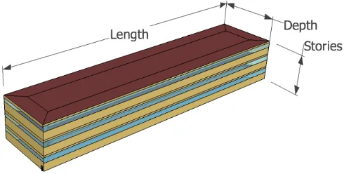
A diagram in plan and 3D view with the relevant geometry parameters is shown in Figure 3.2.
Figure 3.2: Rectangular building with relevant geometry parameters. Aspect Ratio is length divided by depth.
3.1.2 Simulation in EnergyPlus
The number of samples, each representing a unique combination of random draws, must be large enough to adequately cover the decision space created by variations in all parameters. The number of Monte Carlo samples was set at 20,000 to be sufficiently large enough to cover the decision space without detailed analysis to determine the minimum sample size. Simulation of 20,000 energy models in EnergyPlus was run in parallel on a 11-node Linux cluster. Nine of the eleven 11-nodes were available, each with two quad-core processors, which allowed 72 simultaneous EnergyPlus runs, significantly decreasing the model run time. A full annual simulation was run for each energy model. Results for annual heating and cooling load for each sample were compiled and analyzed in MATLAB.
3.1.3 Data Processing
Heating and cooling loads were calculated by EnergyPlus and extracted from the output. These loads represent the amount of energy that must be added to or extracted from the conditioned space to meet the thermostat settings. The heating and cooling loads were adjusted by the efficiency or coefficient of performance (COP) to obtain estimates of end-use energy consumption by typical equipment. Average values of efficiency and COP of 0.80 and 3.23, respectively, for the Medium Office Building type as defined for the DOE Commercial Reference Building based on ASHRAE 90.1-2004, were applied to the loads. In addition, the heating and cooling energy consumption estimates were summed to obtain total energy use.
€
Total Energy=Cooling Load
COP +
Heating Load
efficiency (3.3)
parameter for that run. The angle of the outward facing normal for each external surface determines its orientation.
Figure 3.3: Diagram that describes the building orientation by cardinal direction.
At the base rotation of 0 degrees, the West, South, East, and North orientations were assigned to sides 1, 2, 3, and 4, respectively, as shown in Figure 3.3. Randomly sampled orientation values were used to assign sides to their correct cardinal direction during post processing according to Table 3.4.
Table 3.4: Equivalent cardinal direction for properties assigned to Sides 1-4 in energy model input. This data is used for transformation to cardinal direction based on each orientation sample.
Cardinal Direction after Data Processing
Building Orientation West South East North
0 to 45° 1 2 3 4
45 to 135° 2 3 4 1
135 to 180° 3 4 1 2
3.2 Regression Analysis
percent of runs were used to test the accuracy of the regression equation to predict actual simulation results. The regression produces linear regression coefficients, which were proportional to each parameter’s sensitivity to energy use. The form of the regression equation to predict heating, cooling and total energy is:
€
y x
(
1,x2,...,xn)
=β0+ βjxjj=1
n
∑
(3.4)where y is the predicted heating, cooling, or total energy, xj are the parameters and βj are the corresponding coefficients. It is important to note that each regression model is implicitly based on the fixed inputs in the energy model as well as the location and weather data used for simulation. When a linear regression is performed for heating, cooling and total energy with respect to the 27 design parameters, there is unexplained variance in the models that limits the certainty of any predictions generated with the regression model. The accuracy of the regression models were improved by adding additional terms to the model. Additional terms considered for inclusion in the regression are each a function of one or more of the 27 parameters included in the original sensitivity analysis. For instance:
€
xnew=x1x2 (3.5)
The form of the regression model stays the same, but the revised multivariate linear regression includes cross product terms. Non-linearities exist due to interactions among parameters in the building model; for example, window SHGC and window area. A unit change in SHGC depends on the amount of window area to which the SHGC change is applied. Another example is a unit change in window to wall ratio having a larger impact on a wall with a large versus a small surface area. The parameters associated with the fenestration objects are especially important in this regard because they play a large role in heat transfer through the building envelope. Additional variables considered for inclusion to capture the interaction between window to wall ratio and other parameters were window area, the product of window-to-wall ratio and wall area as well as U-value and SHGC weighted by the appropriate window area.
direction, which represents a range of 90 degrees. Therefore, interaction between orientation and thermal properties of external walls and fenestration were considered to improve the regression. Orientation was sampled on a uniform distribution between 0 and 180 degrees, but is expected to have a non-linear interaction with energy performance: rotation of 0 and 180 degrees should have similar outcomes, with 90 degrees being the most divergent. Therefore, trigonometric functions of the orientation parameter alone and multiplied by other parameters, including aspect ratio, window area, SHGC, window U-value, and shading were investigated as additional variables in the regression model.
Shading projection factor (the ratio of shading projection to window depth) was also found to cause non-linearities in the model. Shading was converted to projection length by multiplying the projection factor by the window-to-wall ratio, which is linearly proportional to window depth due to the constant width of the windows.
3.2.1 Refining the Regression
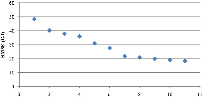
Figure 3.4: Remaining RMSE as a function of the additional included parameters for the heating regression model in Winston-Salem location. Note that the RMSE plotted on the vertical axis is the remaining error after the original 27 design parameters are added to the regression.
Table 3.5: Variables added to heating regression model for Winston-Salem.
Added
Term Variable Name
1 North U-value * Window Area
2 West Window Area
3 East Window Area
4 South Window Area
5 West U-value * Window Area 6 South U-value * Window Area 7 East U-value * Window Area 8 West SHGC * Window Area
9 East SHGC * Window Area
10 South SHGC * Window Area 11 North SHGC * Window Area
are reported for the final regression models tested against the validation set in Table 3.6. For the Miami location, approximately four percent of the validation set had zero annual heating load, which will give infinite percent error for those samples.
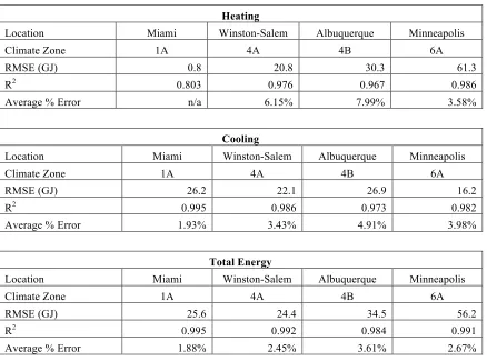
Table 3.6: Validation results for refined regression model using additional terms to capture interactions between parameters and non-linear contributions of parameters
Heating
Location Miami Winston-Salem Albuquerque Minneapolis
Climate Zone 1A 4A 4B 6A
RMSE (GJ) 0.8 20.8 30.3 61.3
R2 0.803 0.976 0.967 0.986
Average % Error n/a 6.15% 7.99% 3.58%
Cooling
Location Miami Winston-Salem Albuquerque Minneapolis
Climate Zone 1A 4A 4B 6A
RMSE (GJ) 26.2 22.1 26.9 16.2
R2 0.995 0.986 0.973 0.982
Average % Error 1.93% 3.43% 4.91% 3.98%
Total Energy
Location Miami Winston-Salem Albuquerque Minneapolis
Climate Zone 1A 4A 4B 6A
RMSE (GJ) 25.6 24.4 34.5 56.2
R2 0.995 0.992 0.984 0.991
Average % Error 1.88% 2.45% 3.61% 2.67%
Overall, the refined regression models show good fit. The heating, cooling, and total energy regression models, when tested with the independent validation set, yielded an R2 greater than 0.96, except for heating in Miami. Interestingly, out of the four locations tested, the R2 for total energy consumption is highest for Miami.
Figure 3.5: Root mean square error (RMSE) observed in heating, cooling, and total energy regression equations when compared to EnergyPlus results in the validation set. The regression for the total energy model consistently shows lower error than the sum of the heating and cooling regressions.
3.3 Parameter Sensitivity
Monte Carlo simulation is also used for sensitivity analysis, and within the regression framework the regression coefficients can be used to provide a relative and quantitative measure of parameter sensitivity. To compare sensitivity of parameters between locations, first an examination of the distribution of EnergyPlus results for each location is discussed. The following section examines the sensitivity analysis results and reports the observations for the four climate locations tested.
3.3.1 EnergyPlus Results
(a)
(b)
(a)
(b)
Figure 3.9: Cooling (a) and heating energy (b) results for the four locations tested. The 10% and 90% quantiles are shown as light and dark boxes, with error bars representing the minimum and maximum observed.
3.3.2 Parameter Sensitivity Methodology
improve model fit, while still keeping each term independent of one another. The units of coefficient βj depend on the units of xj, all of which do not have the same order of magnitude (e.g., building area of 30,000 SF and window solar heat gain coefficient of 0.5). Standardized regression coefficients (SRCs) can be used to compare coefficients with different units. Linear regression coefficients are normalized into SRCs to permit comparison. SRCs are obtained by multiplying each coefficient by the ratio of the estimated standard deviations of
xj to y (Morgan and Henrion 1990 p. 208), as shown in Equation 3.6.
€
USRC
(
xj,y)
=βj×sjsy (3.6)
Normalized values are shown in Table 3.7 for three parameters with respect to Minneapolis heating energy consumption.
Table 3.7: Regression coefficients from multivariate linear regression on heating load for Minneapolis, MN. Standardized regression coefficients (SRCs) permit comparison of coefficients to determine relative sensitivity.
In the Minneapolis results, the building area regression coefficient is relatively small, but the parameter values themselves are large. The opposite can be observed for the window-to-wall ratio and shading projection factor. By normalizing the regression coefficients by the standard deviation of the sampled parameter values, the effects due to the scale of the parameters are eliminated. When comparing the SRCs in Table 3.7, building area is the most sensitive with an SRC of 0.541, followed by window-to-wall ratio with an SRC of 0.306, and only a relatively small contribution by shading projection factor. Note that the standard deviation of a variable that is uniformly distributed is directly proportional to the difference between its minimum and maximum values. Results for the SRCs for heating, cooling, and
6A: Minneapolis Heating Regression, sy = 5.14E+11 J
Parameter Parameter Range [min, max] βj Regression Coefficient sj
Input Std Dev SRC
Area (SF) [20000 , 100000] 1.20E+07 J/SF 23094 SF 0.541
Window-to-Wall
Ratio N [0.02, 0.90] 6.19E+11 J/% Window 0.254 % Window 0.306
Shading Projection
total energy for the four locations are shown in Figure 3.10, Figure 3.11, Figure 3.12, and Figure 3.13.
Figure 3.13: Parameter sensitivity based on the Minneapolis regression model. Parameters are ordered from top to bottom based on their influence on total building energy consumption (labeled ‘Total’).
3.3.3 Results
they both increase the heating and cooling loads for all locations. In Minneapolis, Albuquerque and Winston-Salem, the ranking of window-to-wall ratio by cardinal direction was the same, with North, West, East, and then South in descending order. In Miami, the East, West and South had similar sensitivities, with North being much less sensitive. This is consistent with the trends for cooling in the other locations, which is logical because the total energy in Miami is mostly cooling load. After the shape parameters and the window-to-wall ratio, window properties are the next most sensitive to total heating and cooling energy use. Again sensitivities in Miami differ; SHGC comes next in Miami, while U-value is more significant than SHGC for the other locations. Orientation, or rotation of the building, is generally the next most sensitive parameter following window properties, and in locations with heating (i.e., all but Miami), wall U-value on the north face and roof R-value tend to follow. The results for Miami are somewhat anomalous compared to the other locations, where sensitivities to shading are much higher than window or wall U-value. For Miami, roof color was the sixteenth most sensitive parameter out of 25 parameters, while it had very little effect in the other locations.
Grouping the results for standardized regression coefficients by heating, cooling, and total energy, it is possible to see the trends between climate locations (see Figure 3.14, Figure 3.15, and Figure 3.16 for plots of the most sensitive parameters). With respect to the heating load, SRC results for Minneapolis, Winston-Salem, and Albuquerque are consecutively ordered by either ascending or descending sensitivity for almost all parameters. For example, in Minneapolis greater sensitivity to heating load is observed for building area, aspect ratio, and number of stories. The Winston-Salem location, followed by Albuquerque, has descending sensitivity to these parameters. These parameters all contribute to the heating load, whose effects are exaggerated in colder climates. Window-to-wall ratio and window U-value on the North side have the opposite trend, with Albuquerque being the most sensitive, followed by Winston-Salem and then Minneapolis. This result indicates that the parameters governing the fenestration on the North make a greater contribution to the variability in the heating load in Albuquerque than in Minneapolis.
The standardized regression coefficients are more consistent between locations for the cooling load, as shown in Figure 3.15. Building area dominates the sensitivity of all parameters in all locations. The building area parameter in Albuquerque contributes less to total variability in the cooling load in comparison to other locations. Therefore, sensitivities in the other parameters are higher in Albuquerque, including window-to-wall ratio, shading, and window U-value and SHGC. More detailed analysis of the energy model results are required to understand the contributing factors to this result, but it is worth noting that Albuquerque is the only dry climate tested, and presumably has lower latent cooling load due to ventilation and infiltration at the same outside dry bulb temperature.
Figure 3.15: Standardized regression coefficients for cooling load at all four locations. Parameters are ordered from top to bottom based on their influence on energy consumption in Winston-Salem.
aspect ratio, the number of stories, and the north window-to-wall ratio, similar to the trends for heating.
Figure 3.16: Standardized regression coefficients for total energy consumption (for both heating and cooling) at all four locations. Parameters are ordered from top to bottom based on their influence on energy consumption in Winston-Salem.
While the raw coefficients will have different units and cannot be compared against one another (e.g., window-to-wall ratio and wall R-value), the raw coefficients of the same parameter can be a useful comparison between locations. For example, while the SRC for window U-value on the North side is greatest in Albuquerque, the absolute value of change in heating load in gigajoules per unit change in U-value is not necessarily greatest in
Building Area Aspect Ratio
(a)
He
at
in
g
(b)
Co
ol
in
g
(c)
To
ta
l
Figure 3.17: Comparison of raw linear regression coefficients showing sensitivity of building area and aspect ratio at all four locations. Coefficients are presented for heating (a), cooling (b), and total energy consumption (c).
Window U-value Window-to-Wall Ratio
(a)
He
at
in
g
(b)
Co
ol
in
g
(c)
To
ta
l
3.3.4 Validation
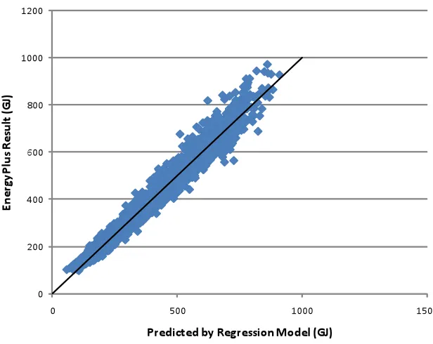
The validation set made up of approximately 20% of the 20,000 samples is used to calculate the error observed by the regression predictions. Error metrics utilized in this analysis include the root mean square error (RMSE), R2, and average percent error for each location. Plots for heating, cooling, and total energy that compare the EnergyPlus simulation result to the value predicted by the multivariate linear regression are shown in Figure 3.19. The various error metrics are reported in Table 3.8.
Table 3.8: Validation results for the multivariate linear regression on heating, cooling, and total energy consumption to obtain SRCs, which measure relative parameter sensitivity.
Heating
Location Miami Winston-Salem Albuquerque Minneapolis
Climate Zone 1A 4A 4B 6A
RMSE (GJ) 1.2 65.4 85.1 222.9
R2 0.498 0.762 0.743 0.816
Average % Error n/a 19.38% 22.80% 12.58%
Cooling
Location Miami Winston-Salem Albuquerque Minneapolis
Climate Zone 1A 4A 4B 6A
RMSE (GJ) 55.0 38.1 46.8 29.0
R2 0.977 0.959 0.917 0.941
Average % Error 4.25% 6.26% 9.23% 7.44%
The regression fits for heating are worse than cooling in all locations. R2 ranged from 0.498 to 0.816 for the heating regression, and from 0.917 to 0.977 for the cooling regression. The regression for total energy yielded an R2from 0.859 to 0.977. The goodness of fit for the
Total Energy
Location Miami Winston-Salem Albuquerque Minneapolis
Climate Zone 1A 4A 4B 6A
RMSE (GJ) 55.1 71.0 91.9 223.2
R2 0.977 0.932 0.886 0.859
3.4 Number of Samples
In this analysis, the 20,000 simulation runs are executed to provide adequate coverage of the decision space. Such a large number of runs are enabled by the available parallel computing capability, which was used to execute 72 simulations simultaneously. This allowed completion of all runs in approximately 13 hours. When conducting the Monte Carlo analysis, the number of samples is typically decided by balancing computational effort with a measure of variability, such as the variance in the mean results (Morgan and Henrion 1990). Past studies using Monte Carlo analysis with building simulation tools have limited the number of runs to a couple hundred or up to 1000 (Burhenne et al. 2010), though many have used very simplified simulation tools. A final step in the analysis involved analyzing the incremental benefit of additional model runs.
The generalized regression equation for the rectangular form in the preceding example is based on a multivariate regression on 80% of 20,000 total samples, or approximately 16,000; the remaining 4,000 samples were used during the validation exercise. The breakdown of total runs into the estimation and validation sets was varied to observe the change in error with fewer samples. Samples were randomly assigned to either the validation or estimation set based on specified probabilities. The probability of being assigned to the estimation set was gradually increased to demonstrate how the error changes as a function of the number of runs used to build the regression model. A Monte Carlo simulation was conducted for Winston-Salem and the results for average error and standard deviation of average error are shown in Table 3.9. In addition, the change in average error versus sample size is shown in Figure 3.20. In each case, the validation set consisted of the remaining samples, or 20,000 minus the number of estimation samples.
Table 3.9: Average and standard deviation of percent error for heating, cooling, and total energy regression models for various sample sizes. Multivariate regression performed with different numbers of samples in the estimation set. Average error and standard deviation of average error based on comparison to the validation set are shown for heating, cooling and total energy load.
Average Percent Error Standard Deviation of Average % Error Number of
Estimation
Samples Heating Cooling Total Heating Cooling Total
62 18.33% 5.87% 6.01% 18.36% 5.08% 5.15%
78 9.91% 4.73% 4.92% 9.47% 4.36% 4.36%
107 9.15% 4.55% 3.43% 8.79% 4.11% 2.97%
210 7.33% 3.78% 2.89% 6.60% 3.43% 2.44%
402 7.00% 3.57% 2.65% 6.28% 3.15% 2.25%
602 6.76% 3.56% 2.56% 5.99% 3.14% 2.14%
802 6.51% 3.50% 2.48% 5.81% 3.08% 2.09%
998 6.53% 3.48% 2.49% 5.89% 3.09% 2.10%
1967 6.34% 3.44% 2.49% 5.66% 3.10% 2.10%
2979 6.32% 3.44% 2.48% 5.65% 3.10% 2.09%
16025 6.15% 3.43% 2.45% 5.47% 3.10% 1.97%
Chapter 4
Discussion
This work was motivated by the lack of building energy information available during early stages of building design. To fill the gap, a simple regression model with predictive capability and a rigorous sensitivity analysis of key building design parameters have been developed. The analysis is based on a generic office building located in four locations:
Miami, Winston-Salem, Albuquerque, and Minneapolis. Remaining questions pertain to how one would use the results in the design process, and what further research could be done to build on this work.
4.1 Use as a Design Tool
The standardized regression coefficients are an indication of sensitivity across the range of each input while varying all other variables simultaneously. All buildings are not perfect rectangles, though many buildings, especially commercial ones are variations of a box. In more complex design situations, approximating a design as a single or multiple rectangular forms could further the usefulness of the regression model, with an appropriate understanding of the effects of the approximations. It is worth pursuing whether such a model based on a specific building type in a given climate location would be useful and insightful to designers. Rank order sensitivities of key parameters could inform design strategy. Such information can yield energy-related insight before starting design or during early design stages. Knowledge of parameter sensitivity can inform design by quantifying tradeoffs between parameters, and focusing attention on the parameters that are most likely to affect the energy goals of the project. The regression model can be used as a quick way to get feedback on early design decisions pertaining to the modeled parameters. With a simple regression equation, different design schemes can be compared against one another.
conceptual design. However, the regression model can quickly show an increase or decrease in energy consumption over a wide range of scenarios and offers a robust technique to analyze tradeoffs between parameters and changes to their values. Parametric analysis could be conducted easily using the regression model to examine one-at-a-time sensitivity. For example, the regression model can be used to examine the effect of increasing the R-value (or decreasing the U-value) of the windows. Two scenarios, one with 30% windows and another with 15% windows computed with the regression model are shown in Figure 4.1
Using the tools developed in this research, early design in mixed climates can provide useful insights. For example, measures commonly considered to be energy efficient (e.g., additional insulation) have mixed effects on heating and cooling. As a result, the effect on annual energy consumption is not always intuitive.
4.2 Further Work
To implement the regression model in the design process, an interface that allows exploration of potential designs and their impact on energy consumption needs to be developed. Formal search techniques can be applied to the regression model to find optimal combinations of parameter values, or to explore multiple near-optimal solutions using the method of modeling to generate alternatives (Brill et al. 1982). Methods to communicate the results and facilitate utilization within design teams needs to be explored. Sensitivity analysis using the regression model can be tailored to specific design questions. For example, if only a few parameters are of interest, sensitivity analysis can be applied to a subset of parameters. Another application is to impose constraints on the ranges of the design parameters and rerun the Monte Carlo simulation to explore the sensitivity within the design decision space available to a specific project. This could be especially valuable because the SRCs can be dependent on the initial range given (Capozzoli et al. 2009), so further refinement of the sensitivities for the portion of design decision space available to a specific project would give better feedback than the generalized sensitivities based on wider ranges.
4.3 Conclusion
In this application, sensitivity analysis and regression analysis are applied to model a rectangular building. Parameters considered include the size and shape, as well as rotation, roof and wall insulation, window R-value, SHGC and shading. Standardized regression coefficients (SRCs) can provide valuable information to designers regarding the relative impact each parameter will have on heating and cooling loads. In the four locations tested—
REFERENCES
ASHRAE. (2007). ANSI/ASHRAE/IESNA Standard 90.1-2007 Energy Standard for Buildings Except Low-Rise Residential Buildings, Atlanta, GA.
ASHRAE. (2011). Advanced Energy Design Guide for Small to Medium Office Buildings. Achieving 50% Energy Savings Toward a Net Zero Energy Building, Atlanta, GA.
Autodesk. (2010). Getting Started with Autodesk Green Building Studio. Autodesk® Ecotect® Analysis 2011, Available at
<http://images.autodesk.com/adsk/files/Getting_Started_with_Green_Building_Studi o_4.3.pdf> accessed 9/20/10.
Bazjanac, V., and Maile, T. (2004). IFC HVAC interface to EnergyPlus-A case of expanded interoperability for energy simulation. IBPSA-USA National Conference, Boulder, CO.
Brill, E.D., Chang, S.H. and Hopkins, L.D. (1982). Modeling to Generate Alternatives: The HSJ Approach and an Illustration Using a Problem in Land Use Planning.
Management Science, 28(3): 221-235.
BuildingSMART. (2010). Model - Industry Foundation Classes (IFC) | buildingSMART. Available at <http://www.buildingsmart.com/bim> accessed 9/22/10.
Burhenne, S., Jacob, D., and Henze, G. P. (2010). Uncertainty Analysis in Building Simulation with Monte Carlo Techniques. Fourth National Conference of IBPSA-USA, New York, NY.
Capozzoli, A., Mechri, H. E., and Corrado, V. (2009). Impacts of architectural design choices on building energy performance applications of uncertainty and sensitivity techniques. Eleventh International IBPSA Conference, Glasgow, Scotland.
Crawley, D.B., Lawrie, L.K., Pedersen, C.O., Liesen, R.J., Fisher, D.E., Strand, R.D., Winkelmann, F.C., Buhl, W.F., Huang, Y.J., and Erdem, A.E. (1999). EnergyPlus Homepage. EnergyPlus: A New-Generation Building Energy Simulation Program. Available at <http://simulationresearch.lbl.gov/EP/ep_paper.html> accessed 6/3/10.
Deru, M., Field, K., Studer, D., Benne, K., Griffith, B., Torcellini, P., Liu, B., Halverson, M., Winiarski, D., Rosenburg, M., Yazdanian, M., Huang, J., and Crawley, D. (2011).
Dong, B., Lam, K.P, Huang, Y.C., and Dobbs, G. M. (2007). A comparative study of the IFC and gbXML informational infrastructures for data exchange in computational design support environments. Proceedings of the 10th Conference on International Building Performance Simulation Association, Beijing, China.
gbXML.org. (2010). About gbXML - Green Building XML Schema. The Open Green Building XML Schema, Inc., Available at http://www.gbxml.org/aboutgbxml.php> accessed 9/20/10.
Hobbs, D., Morbitzer, C., Spires, B., Strachan, P., and Webster, J. (2003). Experience of Using Building Simulation Within the Design Process of an Architectural Practice.
Proceedings of the Eighth International IBPSA Conference, Eindhoven, Netherlands.
Hopfe, C., Hensen, J., and Plokker, W. (2007a). Uncertainty and sensitivity analysis for detailed design support. Proceedings of the 10th IBPSA Building Simulation Conference, Beijing, China.
Hopfe, C., Struck, C., Kotek, P., Schijndel, J., Plokker, W., and Hensen, J. (2007b).
Uncertainty analysis for building performance simulation–a comparison of four tools.
Proceedings of the 10th IBPSA Building Simulation Conference, Beijing, China.
Jacobs, P. and Henderson, H. (2002). State of the Art Review of Whole Building, Building
Envelope, and HVAC Component and System Simulation and Design Tools.
Air-Conditioning and Refrigeration Technology Institute (ARTI), Arlington, VA.
Krygiel, E., and Nies, B. (2008). Green BIM : successful sustainable design with building information modeling. Wiley Pub., Indianapolis, Indiana.
Lam, K.P., Huang, Y.C., and Zhai, C. (2004). Energy Modeling Tools Assessment for Early Design Phase. Center for Building Performance and Diagnostics School of
Architecture, Carnegie Mellon University.
Macdonald, I.A., McElroy, L.B., Hand, J. W., and Clarke, J. A. (2005). Transferring
simulation from specialists into design practice. Proceedings of the 9th International IBPSA Conference, Montreal, Canada.
Morbitzer, C.A. (2003). Towards the Integration of Simulation into the Building Design Process. PhD Dissertation, Department of Mechanical Engineering, University of Strathclyde.
Nielsen, T.R. (2005). Simple tool to evaluate energy demand and indoor environment in the early stages of building design. Solar Energy, 78(1), 73–83.
Rizos, I. (2007). Next generation energy simulation tools: Coupling 3D sketching with energy simulation tools. Masters Thesis, Department of Mechanical Engineering, University of Strathclyde.
Sanguinetti, P., Eastman, C., and Augenbroe, G. (2009). Courthouse Energy Evaluation: BIM and Simulation Model Interoperability in Concept Design. Proceedings of the 11th International IBPSA Conference, Glasgow, Scotland.
Struck, C., Hensen, J., and Kotek, P. (2009). On the Application of Uncertainty and
Sensitivity Analysis with Abstract Building Performance Simulation Tools. Journal of Building Physics, 33(1), 5 -27.
Struck, C., and Hensen, J. (2007). On Supporting Design Decisions in Conceptual Design Addressing Specification Uncertainties Using Performance Simulation. Proceedings of the 10th IBPSA Building Simulation Conference, Beijing, China.
Urban, B.J., and Glicksman, L.R. (2007). A Simplified Rapid Energy Model and Interface for Nontechnical Users. In Proceedings of Oak Ridge National Laboratory,
Buildings Conference X.
Wilcox, S., and Marion, W. (2008). User’s Manual for TMY3 Data Sets Golden, Colorado. National Renewable Energy Laboratory, Golden, CO.
de Wit, S., and Augenbroe, G. (2002). Analysis of uncertainty in building design evaluations and its implications. Energy and Buildings, 34(9), 951-958.
Zhang, Y. (2009). ‘Parallel’ EnergyPlus and the development of a parametric analysis tool.