Evolution of Mutation Rates in Rapidly Adapting Asexual Populations

HIGHLIGHTED ARTICLE

| INVESTIGATION

Evolution of Mutation Rates in Rapidly Adapting

Asexual Populations

Benjamin H. Good*,†,‡_{and Michael M. Desai*},†,‡,1 *Department of Organismic and Evolutionary Biology,†Department of Physics, and‡Faculty of Arts and Sciences Center for Systems Biology, Harvard University, Cambridge, Massachusetts 02138

ABSTRACTMutator and antimutator alleles often arise and spread in both natural microbial populations and laboratory evolution experiments. The evolutionary dynamics of these mutation rate modifiers are determined by indirect selection on linked beneficial and deleterious mutations. These indirect selection pressures have been the focus of much earlier theoretical and empirical work, but we still have a limited analytical understanding of how the interplay between hitchhiking and deleterious load influences the fates of modifier alleles. Our understanding is particularly limited when clonal interference is common, which is the regime of primary interest in laboratory microbial evolution experiments. Here, we calculate thefixation probability of a mutator or antimutator allele in a rapidly adapting asexual population, and we show how this quantity depends on the population size, the beneficial and deleterious mutation rates, and the strength of a typical driver mutation. In the absence of deleterious mutations, wefind that clonal interference enhances the fixation probability of mutators, even as they provide a diminishing benefit to the overall rate of adaptation. When deleterious mutations are included, natural selection pushes the population toward a stable mutation rate that can be suboptimal for the adaptation of the population as a whole. The approach to this stable mutation rate is not necessarily monotonic: even in the absence of epistasis, selection can favor mutator and antimutator alleles that“overshoot”the stable mutation rate by substantial amounts.

KEYWORDSmutator; antimutator; hitchhiking; deleterious load

D

NA replication occurs with extremely high fidelity, de-spite taking place in the noisy environment of the cell. For example, laboratory strains ofEscherichia coliproduce a point mutation at a rate of roughly one nucleotide per 10 billion copied (Wielgosset al.2011; Leeet al.2012), which implies that hundreds of generations can elapse before a single mu-tation is introduced into the genome. To achieve such low error rates, bacteria and eukaryotes employ a complex array of cellular machinery, which must be maintained by natural selection.

One explanation for the low observed error rates is that the genome encodes a large number of functions, all of which are essential for survival. Low mutation rates could then emerge from hard selection against these lethal errors. But, in practice, observed mutation rates lie far below the levels that would quickly result in extinction. This is evident from the fact that mutator strains, whose mutation rates are 10- to 1000-fold

higher than the wild type, can be propagated for thousands of generations in the laboratory without significant loss of via-bility (McDonaldet al.2012; Wiseret al.2013). This suggests that mutation rates are not maintained solely by hard selec-tion, but also by more direct evolutionary competition be-tween strains with different mutation rates. These variants feel the effects of natural selection indirectly, by being linked to other mutations that directly influencefitness.

Strains with higher mutation rates are more likely to be linked to deleterious mutations, and will therefore experience an effectivefitness cost. This cost can be measured in head-to-head competitions between mutator and wild-type strains (Tröbner and Piechocki 1981; Chao and Cox 1983; Chao

et al. 1983; Giraud et al. 2001; Thompson et al. 2006; Gentileet al.2011). In the absence of beneficial mutations,

natural selection will therefore act to decrease the mutation rate, until it is eventually balanced by genetic drift, mutation, or other physiological costs. A large body of previous theo-retical work has explored these dynamics (Kimura 1967; Liberman and Feldman 1986; Dawson 1998, 1999; Johnson 1999a; Lynch 2008; Desai and Fisher 2011; Lynch 2011; Soderberg and Berg 2011; James and Jain 2015).

Copyright © 2016 by the Genetics Society of America doi: 10.1534/genetics.116.193565

Manuscript received July 7, 2016; accepted for publication September 13, 2016; published Early Online September 19, 2016.

1_{Corresponding author: Harvard University, 457.20 Northwest Laboratory, 52 Oxford}

When beneficial mutations are available, lineages with higher mutation rates are also more likely to produce and hitchhike with a successful beneficial variant. In the absence of deleterious mutations, natural selection will therefore act to increase the mutation rate, until the supply of beneficial mutations is eventually exhausted. In accordance with these expectations, mutator alleles are often found to spontaneously arise and spread in rapidly adapting microbial populations in the laboratory (Sniegowskiet al.1997; Notley-McRobbet al.

2002; Shaver et al.2002; Palet al.2007; Voordeckerset al.

2015), and are often correlated with pathogenic lifestyles in the wild (LeClercet al.1996; Maticet al.1997; Oliveret al.

2000; Bjorkholmet al.2001; Denamuret al.2002; Giraudet al.

2002; Richardson et al. 2002; Prunier et al. 2003; Watson

et al.2004; del Campoet al.2005; Labatet al.2005). In a few cases, laboratory populations that have previously fixed a mutator allele have been shown to evolve a lower mutation rate later in the experiment, suggesting that mutation rate evolution is an ongoing process (Tröbner and Piechocki 1984; Notley-McRobb et al. 2002; McDonald et al. 2012; Turrienteset al. 2013; Wielgosset al.2013). Because these populations often continue to increase in fitness during this process (Wielgoss et al. 2013), the success of mutator and antimutator alleles must depend on the interplay between beneficial and deleterious mutations, rather than the complete cessation of adaptation. However, our understanding of this interplay remains incomplete. A few simulation studies have shown how these effects can, in principle, favor either in-creases or dein-creases in mutation rates, depending on the spe-cific population parameters (Taddeiet al.1997; Tenaillonet al.

1999, 2000; Travis and Travis 2002). Some analytical progress has also been made in the case where beneficial mutations are rare, and occur one-by-one in discrete selective sweeps (Leigh 1970, 1973; Painter 1975; Gillespie 1981; Ishii et al. 1989; Kessler and Levine 1998; Johnson 1999b; Tanaka et al.

2003; Andre and Godelle 2006; Wylieet al.2009; Desai and Fisher 2011). However, our understanding is much more lim-ited in larger populations, where beneficial mutations are more common, and multiple adaptive lineages must compete with each other forfixation. This is the regime where the in-direct effects of linked selection are likely to be maximized, and it is also the most relevant for understanding the microbial evolution experiments where mutation rate modifiers have been observed to spread. In this clonal interference regime, even the most basic questions about this process remain unan-swered: exactly how large can the deleterious load be before it effectively selects against a mutator allele? And how does this depend on the population size, the supply of beneficial muta-tions, and the magnitude of the mutator phenotype?

Here, we address these questions in the context of a simple model of adaptation, which is motivated by recent microbial evolution experiments. In particular, we focus on a regime in which deleterious mutations have a negligible impact on the rate of adaptation, even though they may have a large effect on the fates of mutation rate modifiers. Within this model, we calculate thefixation probability of an allele that changes the

mutation rate by a factorr(withr.1 corresponding to muta-tor alleles andr,1 corresponding to antimutators). We con-sider both small changes in mutation rate (r1), as well as substantial changes (wherejlogðrÞj 1).

We find that clonal interference amplifies the beneficial advantage of mutator alleles, even as it constrains the overall rate of adaptation. For largerthis can be a substantial effect, resulting in.100-fold increases in the probability offixation. However, clonal interference also amplifies the effects of the deleterious load, resulting in a much narrower window of mutator favorability. We show that this window depends most strongly on the strengths of typical driver mutations, and relatively weakly on the rate at which beneficial muta-tions arise. With the steady production of such modifier al-leles, the mutation rate will evolve toward a stable point at which neither mutator nor antimutator alleles are favored. Surprisingly, wefind that the approach to this stable point is not necessarily monotonic, even in the absence of epistasis. Instead, alleles that overshoot the stable point can be posi-tively selected, and selection must then act to change the mutation rates in the opposite direction.

Model

Our goal is to understand how beneficial and deleterious mutations influence the fates of mutation rate modifiers in rapidly adapting populations. We focus on the simplest pos-sible model in which we can address this question. Specifically, we consider an asexual haploid population of constant sizeN

(our analysis also applies to diploids when all mutations have intermediate dominance effects). We assume beneficial and deleterious mutations occur at genome-wide ratesUbandUd, respectively. We define U¼UbþUd as the total mutation rate, ande[Ub=Ud as the ratio of beneficial to deleterious mutation rates. We focus on adapting populations, and con-sider both the successional-mutations regime (where benefi-cial mutations are rare), and the clonal interference regime. For most of our analysis, we assume that beneficial mutations all confer the samefitness advantagesb;though we also comment on how our results can be extended to the case where beneficial mutations have a distribution offitness effects. We also assume that there is no macroscopic epistasis among beneficial mutations [as defined by Good and Desai (2015)], so thatUbandsbremain fixed as the population adapts. On sufficiently long timescales, this assumption may eventually break down, so we also comment on the effects of changingUborsbin theDiscussion.

We make no specific assumptions about thefitness effects of deleterious mutations, other than that they are purgeable,

i.e., deleterious mutations are sufficiently costly that they are

unlikely tofix, and do not significantly reduce the overall rate of adaptation of the population. We describe the technical conditions required for this to be true, and the qualitative implications of nonpurgeable deleterious mutations in more detail in theDiscussion.

leavingeandsbunchanged). For simplicity, we assume that this allele has no direct influence onfitness, although in the

Discussion we show how this assumption can be relaxed. These modifier alleles are produced at rate m from the wild-type background, and we assume thatmis sufficiently small that the modifiers can be treated independently. In this case, the substitution rate of the modifier isNmpfixðrÞ;where

pfixðrÞis thefixation probability of a single modifier individ-ual. A natural measure of how selection“favors”or“ disfa-vors”the modifier can be obtained from the scaledfixation probability,NpfixðrÞ:WhenNpfix.1;the allele is favored by selection, since it substitutes more rapidly than a neutral allele; conversely, the allele is disfavored whenNpfix,1:This scaled fixation probability will be our primary focus in the analysis below. In particular, we are interested in determining the parameters where Npfix transitions between favored (Npfix.1) and unfavored (Npfix,1).

We are primarily interested in situations applicable to microbial populations, and particularly to laboratory evolution experiments. This motivates certain technical assumptions we describe in the analysis below. It also motivates our focus on asexual populations where recombi-nation can be neglected. This asexual case is particularly relevant because, when recombination is absent, modifiers of mutation rate remain perfectly linked to the beneficial or deleterious mutations they generate, and hence experience the strongest indirect selection pressures. In principle, we could also apply our analysis to physically linked regions within sexual genomes (“linkage blocks”) that are unlikely to recombine on the appropriate timescales (Neher et al.

2013; Goodet al.2014; Weissman and Hallatschek 2014). However, the scale of these linkage blocks is a complex problem, and understanding these effects is beyond the scope of this study.

In the remaining sections, we calculateNpfixðrÞas a func-tion of the underlying model parameters, and then we use these predictions to analyze the dynamics of mutation rate evolution.

Data availability

The authors state that all data necessary for confirming the conclusions presented in the article are represented fully within the article.

The Successional Mutations Regime

To gain intuition into the forces that determineNpfixðrÞ;it is useful to start by considering the simplest case, where deleterious mutations can be neglected, and adaptation proceeds by a sequence of discrete selective sweeps. This “successional mutations”regime applies whenever bene-ficial mutations are sufficiently rare that they seldom seg-regate within the population at the same time. This will be true provided that NUblogðNsbÞ 1 (Desai and Fisher 2007). In this regime, beneficial mutations are produced at rate NUb and establish with probability

pest¼2sb:Selective sweeps then occur as a Poisson pro-cess with rate

1=test¼2NUbsb: (1) When a successful beneficial mutation establishes, it starts to grow deterministically and requires roughly

Tfix¼ ½ð2=sbÞlogðNsbÞ generations to complete its sweep. By definition, this time is small compared to the time between sweeps, so the rate of adaptation is justy¼sb=test:A modifier allele would increase or decrease this rate by factor ofr, if it was able tofix. We now analyze the dynamics of this process. When a modifier allele first arises, it starts at an initial frequencyfmð0Þ ¼1=N;and it will then drift neutrally until the next selective sweep occurs. Most of the time, the lineage willfluctuate to extinction within thefirst few generations. However, with probability1=t;it will survive fort gener-ations, and reach sizefmðtÞ t=N(Fisher 2007). In the ab-sence of selective sweeps, the modifier lineage can onlyfix by drifting tofixation; this happens with probability1=N, and occurs over a timescale of order N generations. Thus, depending on how this drift timescaleNcompares with the sweep timescalestestandtest=r;two distinct types offixation dynamics can emerge.

Whentestandtest=rare both much larger thanN, then the fate of the modifier lineage will be determined long before the next selective sweep occurs. Drift is the dominant evolu-tionary force, andpfixðrÞ ¼1=N:

In contrast, if eithertestortest=rare small compared toN, thefixation process is instead controlled by genetic draft. In this case, the modifier lineage willfix only if it is lucky enough to produce and hitchhike with the next selective sweep. Since we are primarily interested in understanding these effects, we will focus on this regime for the remainder of our analysis. The next selective sweep is produced by two competing Poisson processes, corresponding to the beneficial mutants from the wild type and modifier lineages. These respectively produce sweeps at rates

l0ðtÞ ¼2NUbsb½12fmðtÞ; (2a)

lmðtÞ ¼2NUbsbr fmðtÞ: (2b) The probability that the next sweep is produced by the modifier lineage is then simply

pfix¼

Z _N

0 l mðtÞe2

Rt

0½l0ðt9Þþlmðt9Þdt9dt

; (3)

where the angled brackets denote an average is over the random lineage trajectoryfmðtÞ:In the regime we are consid-ering, the modifier lineage will remain rare until the next selective sweep occurs. The trajectory fmðtÞis therefore de-scribed by the Langevin dynamics,

@fmðtÞ

@t ¼ ffiffiffiffiffi fm

N r

wherehðtÞ is a Brownian noise term (Gardiner 1985). The solution of Equation (3) can be complicated, since both the overall rate of sweeps and their probability of arising in the modifier lineage depend on the random trajectoryfmðtÞ: We present an exact solution of these equations in Appendix A, using techniques developed by Weissmanet al.(2009).

For the present purposes, however, it will be more useful to focus on an approximation. If the modifier lineage stays sufficiently rare that it does not influence the overall rate of sweeps, then we can approximate l0ðtÞ þlmðtÞ 1=test: Equation (3) then reduces to

pfix¼ Z _N

0

rhfmðtÞie 2t=test

test dt: (5)

In other words, thefixation probability is given by the average size of the lineage at the time of the next sweep, and this time is unaffected by the presence of the modifier. In this case, the modifier lineage is neutral andhfmðtÞi ¼1=N;so that

NpfixðrÞ ¼r: (6)

Thus, we see that the modifierfixation probability (like the proportional change in the rate of adaptation) is independent of the population size, the mutation rate, and the fitness benefits of the driver mutations.

To derive Equation (6), we made the approximation that l0ðtÞ þlmðtÞ 1=test:Substituting our expressions forl0ðtÞ andlmðtÞin Equation (2), we see that this is equivalent to the assumption thatðr21ÞfmðtÞ 1:However, sincefmandtare both random variables, we cannot determine the validity of this assumption based on the average values alone. We must instead consider thetypicaldynamics that contribute to the average in Equation (5): with probability1=test;the modi-fier lineage survives for test generations and reaches size

fmðtestÞ test=N:This ensures that the average size of the lineage is just ½ðtest=NÞ ð1=testÞ ð1=NÞ; as expected. It also shows that the typical values ofðr21ÞfmðtÞwill remain small compared to one provided thatrtestN:For simplic-ity, we will assume that this condition holds for the remainder of our analysis. For moderater, this is actually the same as-sumption we already made in focusing on the genetic-draft regime. For larger, it imposes an upper limitr ðN=testÞ 1 on the range of modifier effects that we consider. However, this is not a fundamental problem for the analysis; we con-sider such large-effect modifiers in Appendix A.

Incorporating purgeable deleterious mutations

A similar picture applies in the presence of strongly deleterious mutations. In particular, we assume that the typicalfitness costs are larger thansb;so that a driver mutation canfix only in a background that is free of deleterious mutations. If the costs are also much larger than Ud;then the vast majority of the population will be of this mutation-free type. We refer to these as purgeable mutations, and we will assume that all deleteri-ous mutations are purgeable in the analysis that follows.

When a new beneficial mutation occurs, the wild type will be in mutation-selection balance with respect to its deleterious muta-tions, so the meanfitness of the population is2Ud:Even if it arises on a mutation-free background, the new beneficial lineage will continue to produce loaded individuals at rateUd:This exactly cancels the growth advantage of the meanfitness of the popu-lation, so that the establishment probability is still just

pest¼2ðsbþUd2UdÞ ¼2sb:Since most genetic backgrounds are in this unloaded state, the overall rate of sweeps is unchanged from before. This means that if a modifier allele were tofix, it would still change the rate of adaptation by a simple factor ofr. However, while the deleterious mutations do not affect the rate of adaptation, they can still have a large effect on the modifier lineage while it is rare. The modifier produces doomed lineages at raterUd;which is not completely can-celled by the meanfitness of the wild type. Instead, mutator alleles will feel an effective cost of magnitude Udðr21Þ; while antimutators will experience an effectivefitness advan-tage. Generalizing Equation (4), the mutation-free portion of the modifier lineage will then evolve as

@fmðtÞ

@t ¼2Udðr21ÞfmðtÞ þ ffiffiffiffiffiffiffiffiffiffi fmðtÞ N r

hðtÞ: (7)

Beneficial mutations produced by this lineage will likewise have an effectivefitnesssb2Udðr21Þ;and will establish with probability

pm_est¼2ðsb2Udðr21ÞÞ: (8)

In exactly the same manner as before, the next selective sweep is produced by two competing Poisson processes with rates

l0ðtÞ ¼

1

test½12fmðtÞ; (9a)

lmðtÞ ¼ r test

12Udðr21Þ

sb

fmðtÞ; (9b)

and thefixation probability is given by the average in Equation (3). If we again make the assumption that the modifier lineage has a negligible influence on the overall sweep rate (lmþl01=test), this reduces to

pfix¼r

12Udðr21Þ

sb

Z _N

0

hfmðtÞie2

t=test

test

dt: (10)

In this case, the average lineage size is now hfmðtÞi ¼

e2Udðr21Þt=_N;_{and we obtain}

NpfixðrÞ ¼ r

12Udðr21Þ

sb

1þUdtestðr21Þ: (11)

considering the typical dynamics behind the averages in Equation (10). These will depend on the sign ofUdðr21Þ:

For a mutator allele (r.1), the modifier lineage will feel

an effectivefitness costUdðr21Þ:If this cost is small com-pared to 1=test;then selection will barely have time to influ-encefmðtÞbefore the next sweep occurs, and mutators will continue to fix with probability Npfixr: On the other hand, ifUdðr21Þ 1=test; then thisfitness cost exponen-tially suppresses the probability that the mutator survives until the next sweep. In particular, the mutator will survive for t1=Udðr21Þ generations with probability Udðr21Þe2Udðr21Þt; and, provided that it does so, it will no longer grow indefinitely, but will instead reach a maxi-mum size of order 1=NUdðr21Þ(Desai and Fisher 2007). If the time between sweeps was deterministic, this would sim-ply suppress thefixation probability by a factore2Udðr21Þtest: However, this is not actually the case, since the next sweep is generated by the random Poisson process described above. In particular, the random nature of this process will occasionally produce a sweep that occurs much earlier thantest:Such anom-alously early sweeps are uncommon, occurring with probability t=test1; but they are far more common than a mutator lineage that survives for a typical sweep time. Combining these facts, we find that the mutator fixation probability is domi-nated by anomalously early sweep times for which

t1=Udðr21Þ test; which leads to a power law decay

NpfixðrÞ}1=Udtestðr21Þ: For a strong-effect mutator (r1), this power-law decay exactly balances the lineage’s increased beneficial mutation rate, so that ther-dependence ofpfixis medi-ated primarily through the reduced establishment probability,pm

est: In contrast, antimutators will have an effectivefitness advan-tage relative to the wild type, of magnitude Udð12rÞ: If

Udð12rÞ 1=test;thisfitness advantage will still have a negli-gible influence onNpfixðrÞ:However, whenUdð12rÞtest1; the antimutator will establish with probabilityUdð12rÞ, and will start to grow deterministically asfmðtÞ eUdðr21Þt=NUdðr21Þ: Again, if the time to the next sweep was deterministic, this would result in a simple exponential enhancement ofNpfix:But because

tis exponentially distributed, it interacts with the exponential growth of the lineage in a strong way. In particular, as

Udð12rÞtest approaches 1, the average in Equation (11) will be dominated by anomalously late sweep times for whichfmðtÞ is no longer rare, and our approximation thatl0þlm1=test breaks down. Thus, Equation (11) will only be valid provided that 12Udð12rÞtest1=logðN=testÞ:Outside this regime, the antimutator lineage will appear to sweep tofixation on its own, without the help of an additional driver mutation.

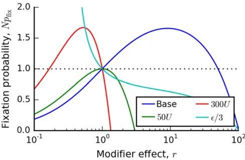
Thefixation probability in Equation (11) is illustrated in Figure 1 for several choices of parameters. Its overall shape is determined by the key parameter

Udtest¼ 1

2eNsb;

(12)

which depends only onN,sb;ande[Ub=Ud;and is indepen-dent of the overall mutation rateU. Depending on the value

of Udtest;Equation (11) takes on one of two characteristic shapes. IfUdtest.1;thefixation probability is a monotoni-cally decreasing function ofr(see Figure 1), and mutators will never be favored to invade. Instead, antimutators will be positively selected. Note that this happens even though the antimutator actually causes a decreasein the overall rate of adaptation.

On the other hand, forUdtest,1;thefixation probability takes on a paraboloid shape (Figure 1). It crossesNpfixðrÞ ¼1 at exactly two points: once atr¼1 and once at

r*¼ sb

Ud

ð12UdtestÞ: (13)

When r*.1; modifiers will be favored in the range 1,r,r*;and disfavored elsewhere (i.e., some mutators will be favored). Conversely, whenr*,1; modifiers will be fa-vored in the ranger*,r,1 (i.e., some antimutators will be favored). It is also useful to rewriter* in terms of the muta-tion rateUm¼Urof the modifier lineage:

Um* [Ur*¼sbð1þeÞ 12 1 2eN sb

: (14)

Note that this is always positive (since 1=2Nsbe,1), and it is independent ofU.

Dynamics of mutation rate evolution

We are now in a position to analyze how mutation rates evolve over time. Imagine that we start with some particular values of

N,U,e, andsb:This will correspond to a particular value of test andU*m:IfUdtest.1;mutators are disfavored and anti-mutator alleles will be positively selected instead. After an antimutator allele fixes, both Ub and Ud are reduced, but

Udtest is unchanged, so natural selection will continue to select for lower mutation rates until this force is balanced by drift, mutational pressure, or other physiological costs.

Figure 1 Thefixation probability of a mutation rate modifier in the suc-cessive mutations regime. Solid lines depict Equation (11) for four sets of parameters, which illustrate the four characteristic shapes ofNpfixðrÞ:In

all four cases, the base parameters areN¼107_;s

On the other hand, ifUdtest,1 andU,U*m;mutators will be favored provided that their resulting mutation rate is less thanU*

m:If a mutator allelefixes,UbandUdwill be increased, butUdtestandUm* will remain constant. Thus, natural selec-tion will continue to favor increased mutaselec-tion rates untilU

reaches a special value,

^

U¼U*

m¼sbð1þeÞ 12 1 2eNsb

; (15)

which is stable against further changes in the mutation rate. If instead the initial mutation rateU.U^;antimutators will be favored provided that their resulting mutation rate is .U^:

Natural selection will then continue to favor decreased mu-tation rates untilUreachesU^:We describe these dynamics in more detail in theDiscussion.

Of course, this analysis crucially depends on the assump-tion that any mutaassump-tion rate increases will still lie within the successive mutations regime. This will be true provided that

NU^beNsb211=logðNsbÞ: But, in order for a nonzero stable mutation rate to exist in thefirst place, we previously required thateNsb1=Udtest.1:These two conditions can be satisfied only if

1 2Nsb,e,

1 2Nsb

1þ 1

logðNsbÞ

: (16)

This is an extremely small region of parameter space, and it grows increasingly narrow asNsb increases. As a result, the stable mutation rate in Equation (15) is actually a rapidly varying function of N,sb;ande. For larger values ofe that violate the stringent constraints in Equation (16), mutator alleles will generically drive mutation rates into regimes where selective sweeps begin to interfere with each other. We now turn to an analysis of this case.

The Clonal Interference Regime

When multiple beneficial mutations segregate at the same time, many potential drivers are lost due to competition with other, fitter genetic backgrounds. This reduces the rate of

successfuldrivers in a way that depends on the relative values ofNsbandNUb:In the regime most relevant for our current study, Desai and Fisher (2007) have shown that test is re-duced to

1 test

2sblogðNsbÞ log2ðsb=UbÞ

; (17)

which is valid provided that 1logðsb=UbÞ 2logðNsbÞ, and 2logðNsbÞ log2ðsb=UbÞ: Similar expressions can be obtained for other parameter regimes, all of which share the weak dependence on NUb (Fisher 2013). Since adap-tation is no longer muadap-tation-limited, one might guess that mutators will be less strongly favored in this regime. How-ever, previous simulation studies (Tenaillonet al.1999) and heuristic reasoning (Desai and Fisher 2011) suggest that the

opposite can actually be true: clonal interference enhances thefixation of mutator alleles, even as they provide a dimin-ishing overall benefit for the rate of adaptation.

In the following subsection, we introduce a traveling-wave formalism for calculating NpfixðrÞ in the presence of clonal interference. Before doing so, however, it will be useful to consider this process from a heuristic perspective. This will allow us to identify the key forces and parameters involved, and will provide intuition for the more rigorous analysis that follows.

Heuristic analysis

In the absence of deleterious mutations, clonal interference alters the dynamics offixation in two main ways. First, success-ful mutations can only occur in the most highly fit genetic backgrounds in the population. These individuals lie in the extreme right tail, or“nose,”of the populationfitness distri-bution, which steadily increases infitness as the population adapts. In the regime described by Equation (17), the relative fitness of the nose is given by

xc 1 test

log

sb

Ub

; (18)

which is much larger than the size of a single driver mutation. These individuals have already acquiredq¼xc=sb1 more adaptive mutations than the average individual, but they are not yet destined to fix. The reason is that there are still enough individuals in the nose that they will collectively pro-duce multiple additional driver mutations in the next test generations, and these will occur in a relatively narrow time windowDttest(Desai and Fisher 2007). By definition, all but one of these mutations must eventually be outcompeted. But this means that the process of fixation within the nose takes place over multiple establishment intervals, each of lengthtest:

Sincexctest1;genetic drift is not directly relevant for most of thisfixation process. Randomfluctuations in the line-age sizes are still important, but these are now driven by

genetic draft, which arises from slight differences in the rela-tive order of the next round of driver mutations. During most of this process, the lineages founded by different driver mu-tations make up less than1=qof the total size of the nose. However, approximately once everyqestablishments, an anomalously early driver mutation will occur and reach an Oð1Þ fraction of the nose (Desaiet al.2013). This roughly coincides with afixation event. In order tofix, a lineage must therefore (i) arise in the nose, (ii) persist forqadditional establishment intervals, and (iii) be lucky enough to hitch-hike with the special“jackpot”driver event.

dynamics as above. The modifier is no more or less likely to arise in the nose compared to a neutral mutation. However, provided that it does occur in one of these special genetic backgrounds, a mutator lineage isrtimes more likely than a neutral lineage to generate an additional driver, while an antimutator lineage isrtimes less likely to do so. Since the modifier lineage must generateqadditional drivers tofix, its overallfixation probability is given by

NpfixðrÞ rq: (19)

Thus, we see that clonal interference increases thefixation prob-ability of mutators byqfactors ofr. This increase can be sub-stantial for larger, even whenq2 (see Figure 2). From our discussion above, we see that this increase is primarily driven by the fact thatmultipleadditional drivers are required forfixation. In the presence of deleterious mutations, a mutator lineage again feels an effective cost of Udðr21Þ;so it will tend to decline in frequency relative to the other individuals in the nose. In particular, when the next burst of driver mutations arises, the mutator lineage will have decreased in frequency by a factor ofe2Udðr21Þtest;_{which makes it that much less likely} to survive to the next round. Similarly, an antimutator lineage will have increased in frequency by an analogous factor of

eUdð12rÞtest:_{The overall}fixation probability then becomes

NpfixðrÞ re2ðr21ÞUdtest q

: (20)

We discuss the regimes of validity of this expression in our more rigorous analysis below. For the purposes of our heuristic analysis, it will be more useful to focus on the implications of Equation (20).

Similar to the selective sweeps case, the direction of selec-tion in Equaselec-tion (20) is again determined by the product

Udtest: There are three characteristic regimes of behavior. When Udtest1; mutators will be favored provided that

Um¼Uris less than a maximum value,

U*

m¼ 1þe test

log

1

Udtest

; (21)

which corresponds to the largest value of r for which

NpfixðrÞ.1:Conversely, whenUdtest1;antimutators will be favored above a minimum value

Um* ¼ 1þe

test

Udteste2Udtest: (22)

Similar behavior is obtained forUdtestis close to one, except thatU*

mis now given by

U*m¼U

1þ12Udtest 2

: (23)

WhenUdtest¼1;the range of favorable modifiers vanishes, and mutators and antimutators are both selected against. The evolutionarily stable mutation rate is therefore given by

^

U¼1þe test :

(24)

Note that this is actually an implicit relation forU^;sincetest depends onU^b¼eU^=ð1þeÞ:Substituting our expression for testin Equation (17), and solving forU^;wefind that

^

U 2sblogðNsbÞ

log2 1_e ; (25)

where the region of validity for Equation (17) [and hence Equation (25)] now becomes

1 ffiffiffiffiffiffiffiffiffiffiffiffiffiffiffiffiffiffiffiffi2logðNsbÞ

p

log 1ð =eÞ 2logðNsbÞ: (26)

This is still a restrictive parameter range fore, although it is much broader than Equation (16) in the successive mutations regime, and it grows larger with increasingNsb:

Provided that these conditions are met, we see that the stable mutation rate in Equation (25) is only weakly depen-dent onNande, and is much more strongly influenced bysb:

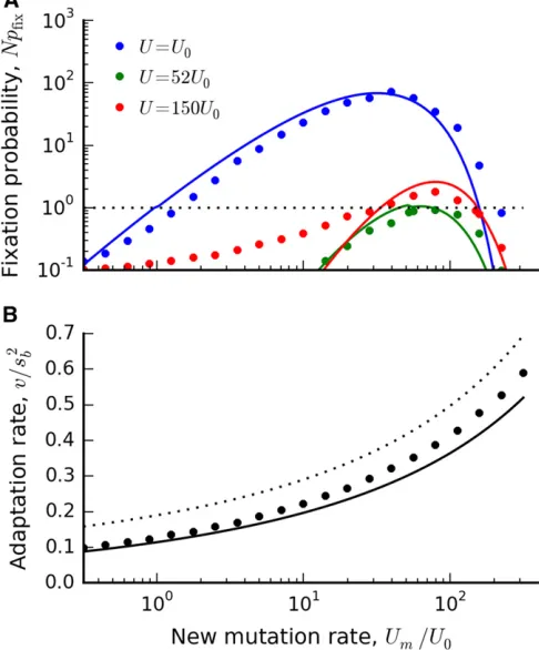
Figure 2 (Top) Thefixation probability of a mutation rate modifier in the clonal interference regime whenUd¼0:Symbols denote the results of forward-time solutions (described in Appendix C) for sb¼1022; Ub¼1025;andN2 f105;107;109gSolid lines denote the theoretical predictions in Equation (38). For comparison, the successive muta-tions prediction (Npfixr) and neutrality (Npfix1) are shown by the

dashed lines. (Bottom) The rate of adaptation of a successful modifier lineage, relative to that of the wild type, for the same set of popula-tions above. The solid black line denotes the asymptotic prediction,

This contrasts with the behavior we found in the successive mutations regime. In addition, we see that, unlike in the successive mutations regime, the stable mutation rate (U^) does not necessarily coincide with the maximally permitted mutator or antimutator allele (U*_{m) when U6¼U}^_{:This can} have important consequences for the dynamics of mutation rate evolution in this regime. If the mutation rate starts far above or belowU^;natural selection can favor modifier alleles

that overshoot the stable value by a substantial amount, which can lead to a nonmonotinic approach to the stable point. We will revisit these dynamics in more detail in the

Discussion.

Formal analysis

We now turn to a more formal derivation of the results de-scribed above. To do so, we make use of “traveling-wave” formalism developed in previous work (Tsimring et al.

1996; Rouzine et al. 2003; Neheret al. 2010; Hallatschek 2011; Neher and Shraiman 2011; Goodet al.2012; Fisher 2013; Good and Desai 2014). This formalism focuses on the distribution of relative fitness within the population, which we denote by fðxÞ;and the fixation probability of a (wild-type) individual with relativefitnessx, which we denote by

wðxÞ: In the absence of mutator or antimutator alleles, we and others have previously shown thatfðxÞandwðxÞsatisfy the partial differential equations,

2y_@@f

x¼ ðx2Ud2UbÞfþUbfðx2sbÞ; (27a)

y@_@w

x¼ ðx2Ud2UbÞwþUbwðxþsbÞ2 w2

2; (27b)

wherey[sb=testis the average rate of adaptation (Good and Desai 2014). Note that Equation (27) implicitly assumes that the deleterious mutations are purgeable,i.e., they do notfix, and constitute a negligible fraction of the population. The rate of adaptation (or equivalently,test[sb=y) is set by the self-consistency condition,

Z

fðxÞwðxÞdx¼1

N; (28)

which is just another way of saying that thefixation prob-ability of a neutral mutation must be equal to 1=N:For a detailed derivation of these equations, see Good and Desai (2014). Note that, because we have assumed that deleteri-ous mutations are purgeable,Udenters into Equations (27) and (28) only as an overall shift in the meanfitness of the population. If we measurefitnesses using the shifted vari-able~x¼x2Ud(i.e.,fitness relative to the averageunloaded individual), then the evolution equations revert back to the purely beneficial case. We will adopt this convention from now on.

Even in the simplified model of Equation (27), there are many possible parameter regimes that one may consider (Fisher 2013). Here we will focus on a particular approximate

solution (based on ideas introduced in earlier studies by Tsimringet al.(1996), Neheret al.(2010), and Hallatschek (2011)), which is thought to be relevant for many microbial evolution experiments (Desaiet al.2007; Perfeitoet al.2007; Wiseret al.2013; Barroso-Batistaet al.2014). In this regime, thefitnesses of unloaded individuals are approximately nor-mally distributed,

f~x ffiffiffiffiffiffiffiffiffi1

2py

p e2x22yu x_c2~x

; (29)

with a sharp cutoff at~x¼xc:This corresponds to the“nose”of thefitness distribution described above. Meanwhile, the sur-vival probabilitywð~xÞcan be approximated by the piecewise form

w~x

2~x if ~x.xc; 2xce

x2₂x2

c

2y if x_c2s_b#~x#x_c; 0 if ~x#xc2sb:

8 > > < > >

: (30)

In this context,xc can also be thought of as aninterference

threshold. Lineages that are at relativefitnessx.xcwillfix provided they survive drift and establish; this occurs with probability 2x:Below xc, the fixation probability drops off rapidly because lineages can establish but still be lost to in-terference. Once a lineage is more thansbbelow xc;it can essentially never catch up with the remaining lineages at the nose, and it will therefore have a negligiblefixation proba-bility. The location of xc is determined by the auxiliary condition

1Ub

sb

12sb

xc

₂1 excsby2

s2

b

2y: (31)

After substituting our expressions for fðxÞ and wðxÞ into Equation (28), the self-consistency condition becomes

2xcsbe2 x2

c

2y

ffiffiffiffiffiffiffiffiffi

2py

p 1

N: (32)

Together with Equation (31), this completely determines v

andxcas a function of the underlying parameters. Asymptotic formulae for these quantities are given in Equations (17) and (18); more accurate estimates can be obtained by solving Equations (31) and (32) numerically.

We have previously shown that this solution applies when-ever xc2sb ffiffiffiy

p

;sb ffiffiffiy p

Once we have set up this traveling-wave formalism, mutation-rate modifiers can be added in a straightforward way. Since the fate of any allele is determined while it is rare, we can neglect the effects of the modifier on the wild-type pop-ulation, so thatfðxÞandvare unchanged from above. When a modifier allele occurs, it will arise on a genetic background whose fitness is drawn fromfðxÞ:We then introduce a new function,wmðxÞ, describing thefixation probability of the mod-ifier allele as a function of its initialfitness. This function satisfies a similar equation aswðxÞ;except with a different mutation rate:

y@_@w_~m x ¼

h

~

x2ðr21ÞUd2rUb

i wm

þrUbwm

~

xþsb

2w2m

2 :

(33)

Thus, in addition to the increase inUb;we see that a mutator lineage experiences an effectivefitness cost Udðr21Þ corre-sponding to its increased deleterious load. This cost enters as a shift in the overall location ofwmð~xÞ;which we can account for by defining a shifted function, wmð~xÞ ¼w~mð~x2Udðr21ÞÞ: After this transformation, Equation (33) is of the same form as Equation (27b). Then, provided that the modifier mutation raterUbis still in the same regime asUb;the solution for the shifted functionw~mð~xÞwill have the same form aswð~xÞ;

~

wm

~

x¼

2~x if ~x.xcm; 2xcme

x22x2_cm

2y if x_cm2s_b#~x#x_cm; 0 if ~x#xcm2sb;

8 > > < > > :

(34)

except with a different interference threshold, xcm; which satisfies

1¼rUb

sb

12sb

xcm

₂1 excmsby 2

s2_b

2y: (35)

Like the wild-type interference thresholdxc;the location ofxcmis independent ofUd:Since mutators are favored whenUd¼0;we expect thatxcm,xcwheneverr.1:In other words, we expect that mutators have a lower interference threshold, since these lineages generate beneficial mutations more rapidly and, once in the nose, are therefore less likely to be lost to clonal interference. In order for this solution to apply, it must satisfy the same conditions as the wild-type population: xcm2sb ffiffiffiy

p and

rUbsb:This will be true provided thatxcm is still close to xc; or, equivalently, that the fractional difference dx¼xcm=xc21 is small compared to 1. Given this assumption, we can divide Equation (35) by Equation (31), and solve fordx:

dx¼ 2 y

xcsb

log rð1þdxÞ 1þ xcdx

xc2sb

2 6 6 4

3 7 7

5 2_xcy_sblogðrÞ: (36)

Sincexcsb=ylogðsb=UbÞin this regime, we see that this ap-proximation will hold provided that jlogðrÞj logðsb=UbÞ:

This places an upper limit on the range of modifier effects that we can consider. But sincesb=Ub1;this includes many realistically large modifiers of orderr100:

Given our solution for wmð~xÞ;we can compute the mar-ginal fixation probability of the modifier by averaging over all the fitness backgrounds that the modifier could have arisen on:

pfixðrÞ ¼ Z

f~xwm

~

xd~x: (37)

We evaluate this integral in Appendix B. Wefind that

NpfixðrÞ eq½logðrÞ2Udtestðr21Þ3 e2

n

2½logðrÞ2Udtestðr21Þ2

3eUdtestðr21Þ21 Udtestðr21Þ;

(38)

where we have employed the short-hand notationq¼xc=sb; test¼sb=y;andn¼1=sbtest:In the asymptotic regime we are considering, 1=qandnare both small parameters. To leading order, Equation (38) converges to the simpler expression from our heuristic analysis, which we now recognize as the technical statement that

lim q/N

n/0

logNpfixðrÞ

q ¼logðrÞ2Udtestðr21Þ: (39)

However, since the errors are multiplied by a large numberq

and exponentiated, the full version in Equation (38) is often required for quantitative accuracy.

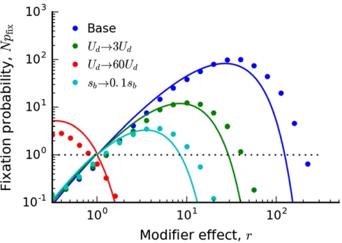
We illustrate the full expression in Equation (38), and compare it to forward-time simulations in Figure 2 and Fig-ure 3. The accuracy is generally good, although there are some systematic deviations for large rwhen the effects of the deleterious load are particularly costly. These are ulti-mately the result of two factors: (i) inaccuracies in our ap-proximate solution for wðxÞ forxc2sb,x,xc, and (ii) the fact that logðrÞis starting to approach logðsb=UbÞ:More accu-rate approximations forwðxÞderived by Fisher (2013) could be used to improve the quantitative accuracy for these pa-rameters; we leave this for future work.

Discussion

that neither mutators nor antimutators are favored. We now consider how a population will approach the stable mutation rate, and the implications of this mutation rate evolution for the rate of adaptation within the population. Finally, we de-scribe the approximations we have made throughout our analysis and the resulting limitations of our approach.

Approach to the stable mutation rate

Consider a situation in which the population starts with a mutation rateU06¼U^;andfixes a sequence of modifier alleles with mutation ratesU1;U2;. . .;Un:What are the typical val-ues of this mutation rate trajectory, under the hypothesis that each step was favored by selection?

In both the successional mutations and clonal interference regimes, we found thatU^depends only onN,sb;ande. This implies that the mutation rate will always evolve toward this unique stable point:Un/U^:However, the manner in which the population approachesU^ can be strongly influenced by

clonal interference.

In the successional mutations regime, selection favors a monotonic approach to U^: Consider, e.g., a mutation rate

U0,U^:In this case, we have shown that mutators will be able tofix, provided that the new mutation rateUm¼rUlies in the rangeU0,Um,U^:When one of these allelesfixes, the new mutation rate will be given byU1 ¼Um;and the process will repeat itself. Mutators will still be favored tofix provided thatU1,Um,U^;which will lead to aU2.U1;and so on. Thus, evolution will favor a monotonic sequence of mutator alleles until Un¼U^;after which the mutation rate will be stable to further changes. An exactly analogous conclusion holds if U0 starts aboveU^: here, selection will tend tofix antimutator alleles that lie in the range U^,Um,Ui until

Un¼U^:In both cases, mutator or antimutator alleles that “overshoot”the stable mutation rate are always disfavored. This is true even if such alleles would move the mutation rate closer to the stable rate;e.g., an allele that takes a population from 0:1U^/1:1U^ would not be positively selected.

When clonal interference is present, the approach to the stable mutation rate is more complex. This is easiest to see if we rewrite Equation (20) in terms ofUm;U, andU^:Provided thatjlogðUi=U^Þj logð1=eÞ;the quantitiestestðUÞandqðUÞ will stay roughly constant over the relevant range of muta-tion rates, and we can approximatetestðUÞ testðU^Þ[1=U^: This yields a simple heuristic formula,

NpfixðUmÞ

Ume2Um=U^

Ue2U=U^ !q

; (40)

which depends only on the scaled mutation ratesU=U^;Um=U^; andq. A more accurate (but more cumbersome) version can be obtained by substituting the full expressions for testðUÞ andqðUÞinto Equation (38). We illustrate this full expression in Figure 4 for a particular combination ofNsbande, although the important qualitative features are already contained in Equation (40).

If the population starts at a mutation rateU0U^;then only modest changes in the mutation rate will be favorable. However, if the population starts at a mutation rateU0U^; Equation (40) shows that mutators will be positively se-lected, provided thatU0,Um,U^logðU^=U0Þ:While the most strongly beneficial modifier hasUm¼U^;the range of favored mutators also includes values ofUmthat arelargerthanU^by a factor logðU^=U0Þ 1: This means that selection can fa-vor mutator alleles that overshoot the stable mutation rate by a substantial amount. If a mutator allele of this maximal strength fixes, the new mutation rate will be

U1¼U^logðU^=U0Þ.U^;and selection will immediately favor thefixation of antimutator alleles, despite the fact that the location ofU^ has not changed (see Figure 4 and Figure 5). If UU^; these antimutator alleles can overshoot the stable mutation rate in the other direction, by a factor

U=Ue^ 2U=U^ _{1:In the example above, this could then lead}

toU2¼U0logðU^=U0Þ;which is larger than the initial muta-tion rateU0 but still much smaller thanU^:Thus, while the population will still approach the stable mutation rate over time, this approach does not have to be monotonic, even in the absence of epistasis or environmental variation. More-over, the functional form of Equation (40) implies that this behavior is highly asymmetric: an antimutator allele can overshootU^by a larger amount (and with a largerNpfix) than a mutator allele with the same value ofjlogðU=U^Þj:This can also be seen in Figure 4 and Figure 5.

Application to a long-term evolution experiment in E. coli

Several studies have observed the spread of mutator alleles in microbial populations in the laboratory. One of the best-studied examples is Lenski’s long-term evolution experiment (the LTEE), where 12 replicate populations of E. coli have

Figure 3 The fixation probability of a mutation rate modifier in the clonal interference regime when Ud.0: Symbols denote the results of forward-time simulations with the base parameters N¼107_;

been propagated under constant conditions for more than 60;000 generations (Lenskiet al.1991, 2015). Mutator phe-notypes have fixed in six of the 12 populations over the course of this experiment, and have typically increased the mutation rate by100-fold. The rate of adaptation in the mutator populations increased less than twofold, sug-gesting that clonal interference plays an important role (Wiseret al.2013). In one of the 12 replicates, the dynamics of mutation rate evolution have been studied in more detail. Wielgosset al.(2013) have shown that, soon after the fix-ation of the mutator allele, an antimutator phenotypefixed, which lowered the mutation rate by a factor of approxi-mately two. The antimutator phenotype had two inde-pendent origins, suggesting that both it and the original mutator allele were favored by selection. Given these find-ings, it is interesting to compare various explanations for this behavior in the context of our theoretical analysis above.

One potential explanation for thesefindings is suggested by the“overshooting”behavior illustrated in Figure 4 and Figure 5. Although the precise evolutionary parameters of these populations are not known, Figure 5 shows that it is at least feasible to overshoot the optimum by a factor of 2 when the population starts at a mutation rate of U0 0:01U^: Note, however, thatNpfixis not necessarily large in the reverse di-rection, so it remains to be seen whether this effect could efficiently select for lower mutation rates on the rapid time-scales observed.

Another potential explanation for the mutation-rate re-versal, initially suggested by Wielgosset al.(2013), is that long-term epistasis reduced the effective advantage of hitch-hiking later in the experiment, thereby shifting the location of

^

Ubelow its initial value. Our analysis above does not account for these effects directly, since it assumes a constant value of eandsb:However, as long as any epistasis manifests itself on timescales that are longer than thefixation time, we can still

account for these effects in a crude way by examining howU^

changes after a shift inUborsb:For example, epistasis could lead to a reduction in e, reflecting a diminished supply of beneficial mutations (or an increasing supply of deleterious mutations) as the population adapts. Due to the presence of clonal interference, Equation (25) suggests that rather dras-tic reductions ineare required to cause a twofold reduction in

^

U: Alternatively, diminishing-returns epistasis could reduce the magnitude of sb;while leaving the beneficial mutation rate unchanged. Equation (25) suggests that this has much stronger effect on U^:Wiseret al.(2013) have recently pro-posed andfit a concrete model for howsb declines with fit-ness in the LTEE. These estimates suggest thatsbdeclines by ≲20% in the 4000 generations that separate the mutator and antimutator alleles. This would seem to be too small to ac-count for a ≳50% reduction inU^;although the magnitudes are sufficiently close that a careful comparison with simula-tions is required. This would be an interesting avenue for future work.

A third potential explanation is a direct fitness benefit to either the mutator or antimutator allele. While such

Figure 4 The predicted fixation probability of a modifier allele when

Nsb¼106ande¼1026:Grid points are colored according to the value of Npfix from Equation (38), and are capped at a maximum value of jlog2Npfixj ¼2 to maintain contrast. For comparison, the solid lines

de-note 20 log-spaced contours that range from 1021_{to 10}4_:

Figure 5 (Top) A vertical“slice”of Figure 4 for three different values of U. Symbols denote the results of forward time simulations with

NU0¼5780;andsd¼5sb;other parameters are the same as Figure 4. Solid lines denote theoretical predictions from Equation (38). (Bottom) The scaled rate of adaptation as a function of the mutation rate for the same set of parameters. Symbols denote the results of forward-time simulations, the solid lines show the theoretical predictions obtained by solving Equations (31) and (32) numerically, and the dashed line shows the asymptotic formula,v=s2

benefits are difficult to measure directly (due to the con-founding effects of the deleterious load), they can be in-corporated into our model in a straightforward way. We can simply replace Udðr21Þ/Udðr21Þ2sm in our formulae for pfixðrÞ; where sm is the direct benefit of the modifier allele. Since the effect of the deleterious load is typically of order U^,sb; even a small direct benefit (sm,sb) can shift the balance between hitchhiking and load in impor-tant ways.

The evolution of mutation rates and the average rate of adaptation

Because we have assumed that deleterious mutations are purgeable, increasing Ualways increases the rate of adap-tation, even though these increases may be small in the presence of clonal interference. Our results therefore sug-gest that mutation rates will evolve toward a stable muta-tion rate that is less than what would be optimal for the population (which, in this case, is technically Uopt¼N). Of course, as we increase mutation rates, the assumption that deleterious mutations are purgeable will eventually fail. Somewhere above this point, there will be an optimal mutation rateUopt,Nthat maximizes the rate of adapta-tion [see,e.g., Orr (2000)]. To confirm that the stable

mu-tation rate is indeed belowUopt;we must verify thatU^is still in the purgeable deleterious mutations regime. For the ex-ample in Figure 5, we can verify this directly, since the rate of adaptation continues to increase as the mutation rate passes throughU^:This behavior will hold more generally provided that the typical cost of a deleterious mutation,sd;is much larger thanU^:SinceU^ is typically smaller than sbin the regimes that we consider, this will indeed be the case wheneversd≳sb:

In these cases, the stable mutation rate is below the optimal mutation rate, which implies that the dynamics of the evolu-tionary process can sometimes favor changes in mutation rate that slow the adaptation of the population. Antimutator alleles can be favored even when theirfixation will ultimately reduce the overall rate of adaptation. Conversely, mutator alleles can be disfavored even when theirfixation would have increased the rate of adaptation.

Although our results are limited to the purgeable regime, a similar distinction betweenU^ andUoptmay also apply even when deleterious mutations are no longer purgeable. We cannot prove this conjecture in our present framework, but it is an interesting hypothesis for future work.

Limitations to our analysis

We have made a number of key assumptions throughout our analysis. Most crucially, we have assumed that deleterious mutations are purgeable. For this to be true, two conditions must be met: the deleterious mutations cannot fix, nor can they affect the overall rate of adaptation by reducing the fixation probabilities of beneficial mutations. This is a slightly stronger condition than the“ruby in the rough” approximation used by earlier authors (Charlesworth

1994; Peck 1994). Our previous work on the effects of deleterious mutations in adapting populations provides a detailed analysis of when these conditions will hold, and of the effects of deleterious mutations on adaptation when the purgeable assumption fails (Good and Desai 2014). This earlier work suggests that deleterious mutations are likely to be purgeable in most microbial evolution experi-ments, though recent experimental work hints that this may not always be the case (McDonaldet al.2016). Here, wefirst summarize the conditions under which deleterious mutations are purgeable, and then describe the potential effects of deleterious mutations when this condition is violated.

In our earlier work, we showed that deleterious mutations with fitness cost sd will typically not fix provided that

sd1=Tc; where Tcqtest is the coalescence timescale (Good and Desai 2014). Since sb1=Tcin all the regimes that we consider, this will be true provided thatsdis not much smaller than sb:Deleterious mutations can also hinder the fixation of beneficial mutations that arise in less-fit back-grounds. However, provided thatsdUd;deleterious vari-ants will be rapidly eliminated from the population, and most genetic backgrounds will be free of deleterious mutations. Assuming typical values of Ud1024 and

sd102221021for microbial evolution experiments (Wloch

et al.2001), this condition will often be met.

In addition to these key limitations of our analysis, we have also made a number of more technical assumptions. For example, we have assumed that beneficial mutations all pro-vide the samefitness benefit,sb:In reality, beneficial muta-tions will have a range of differentfitness effects, drawn from some distribution. However, earlier work has shown that in this case the evolutionary dynamics can often be summarized using a single effective beneficial fitness effect, and corre-sponding effective beneficial mutation rate (Desai and Fisher 2007; Good et al. 2012; Fisher 2013). Thus our analysis can be applied to this situation using the appropriate effective

sbandUb:

In our analysis of clonal interference, we focused on a regime in which 1logðsb=UbÞ 2logðNsbÞ log2ðsb=UbÞ:The lat-ter condition implies that clonal inlat-terference is not excep-tionally strong, and is often a good approximation for microbial evolution experiments at wild-type mutation rates. For some large effect mutators, we start to approach the boundary of this regime, and our quantitative expres-sions become less accurate (see Figure 5). In princi-ple, we could extend our analysis to the “high-speed” [2logðNsbÞ log2ðsb=UbÞ] or “mutational-diffusion” re-gimes [Ubsb] by using analogous solutions forfðxÞand

wðxÞderived by Fisher (2013) or Hallatschek (2011). We leave this for future work.

Throughout our analysis, we have assumed that modifier effect sizes can be large but not exceptionally so [e.g., in the clonal interference regime, jlogðrÞj logðsb=UbÞ]. Since

Ubsb; this includes many realistically large mutators of order r100; and, in practice, our expressions appear to work reasonably well even when logðrÞ logðsb=UbÞ (see Figure 3). For sufficiently large r, we may also encounter situations where modifiers switch from one regime to an-other (e.g., from the clonal interference to successive mutations regime, or fromUbsbtoUb.sb). Our quanti-tative predictions forNpfixbreak down in all of these cases. However, the evolutionarily stable mutation rates are de-fined by the behavior ofNpfixin the local neighborhood of

r1;so the location ofU^is not influenced by this problem.

If the population starts sufficiently far from U^; then the fixation probabilities of thefirst few Ui are not well-described by our analysis, but we know that the mutation rate must still approach U^ (in a possibly nonmonotonic manner). Eventually, the mutation rate will become close enough to U^ that our expressions start to apply, and the remaining steps of the mutation trajectory can be predicted.

Finally, we have assumed throughout that modifier mu-tations are sufficiently rare that their fates are deter-mined independently. In other words, we have neglected clonal interferencebetweendifferent modifier mutations.

For deleterious or weakly beneficial modifiers, this will often be a good approximation. However, for strongly beneficial modifiers, this requires that the establishment time 1=NmpfixðrÞ between successive mutators is large compared to the fixation time. In the clonal interference

regime, Tfixlogðsb=UbÞ=sb; and this condition becomes msb=logðsb=UbÞNpfixðrÞ: This can sometimes be violated for strongly beneficial mutator alleles with a large target size (e.g., loss-of-function mutations in multiple genes). In these cases, our quantitative predictions become inaccurate, al-though the overall direction of selection [i.e., whether

Npfix.1 orNpfix,1] will remain unchanged.

Conclusions

Our analysis has explained how the interplay between beneficial and deleterious mutations in adapting popula-tions creates indirect selection pressures on modifiers of mutation rates, and we have shown how these indirect selection pressures affect the fates of mutator and antimu-tator alleles. Our analysis of the successional mutations regime follows the logic of earlier work (Andre and Godelle 2006; Desai and Fisher 2011), balancing the probability a new beneficial mutation arises in a mutator, or antimuta-tor, background with the effects of the modifier allele on the accumulation of deleterious load. We have also studied rapidly adapting populations where clonal interference is widespread. Our approach to this question builds on the traveling wave framework we and others have recently introduced (Neher et al. 2010; Hallatschek 2011; Neher and Shraiman 2011; Goodet al.2012; Fisher 2013; Good and Desai 2014). In this framework, analyzing the fate of an allele modifying mutation rate is similar in spirit to calculating thefixation probability of any lineage: we must solve the same equation forwðxÞ;except instead of a mu-tation changing thefitnessx, it changes the mutation rate

U. This general framework can also be applied to analyze indirect selection pressures that act on other modifiers of the evolutionary process. For example, we could analyze the fate of a mutation that changes the distribution of fit-ness effects of new mutations by solving for wðxÞ for an allele that modifiesrðsÞ:Our analysis does not need to be limited to adapting populations, since the traveling wave framework applies whenever interference selection is widespread, even if the population is not adapting on av-erage. Of course, in practice, some modifiers and parameter regimes will lead to equations forwðxÞthat are analytically tractable, while others will not. Thus further work is needed to more fully understand both the limits and promise of this approach.

Acknowledgments

Literature Cited

Andre, J.-B., and B. Godelle, 2006 The evolution of mutation rate in_finite asexual populations. Genetics 172: 611_–626.

Barroso-Batista, J., A. Sousa, M. Lourenço, M.-L. Bergman, J.

Demengeot et al., 2014 The _first steps of adaptation of

Escherichia coli to the gut are dominated by soft sweeps. PLoS Genet. 10: e1004182.

Bjorkholm, B., M. Sjolund, P. G. Falk, O. G. Berg, L. Engstrandet al., 2001 Mutation frequency and biological cost of antibiotic re-sistance in Helicobacter pylori. Proc. Natl. Acad. Sci. USA 98: 14607_–14612.

Chao, L., and E. C. Cox, 1983 Competition between high and low mutating strains ofEscherichia coli. Evolution 37: 125_–134. Chao, L., C. Vargas, B. B. Spear, and E. C. Cox, 1983 Transposable

elements as mutator genes in evolution. Nature 303: 633_–635. Charlesworth, B., 1994 The effect of background selection against deleterious mutations on weakly selected, linked variants. Genet. Res. 63: 213_–227.

Dawson, K. J., 1998 Evolutionarily stable mutation rates. J. Theor. Biol. 194: 147–157.

Dawson, K. J., 1999 The dynamics of infinitesimally rare alleles, applied to the evolution of mutation rates and the expression of deleterious mutations. Theor. Popul. Biol. 55: 1–22.

del Campo, R., M. I. Morosini, E. G. G. de la Pedrosa, A. Fenoll, C. Munoz-Almagro et al., 2005 Population structure, antimicro-bial resistance, and mutation frequencies ofStreptococcus pneu-moniae isolatesfrom cysticfibrosis patients. J. Clin. Microbiol. 43: 2207–2214.

Denamur, E., S. Bonacorsi, A. Giraud, P. Duriez, F. Hilali et al., 2002 High frequency of mutator strains among human uropa-thogenicEscherichia coliisolates. J. Bacteriol. 184: 605–609. Desai, M. M., and D. S. Fisher, 2007 Beneficial mutation selection

balance and the effect of genetic linkage on positive selection. Genetics 176: 1759–1798.

Desai, M. M., and D. S. Fisher, 2011 The balance between muta-tors and nonmutamuta-tors in asexual populations. Genetics 188: 997–1014.

Desai, M. M., D. S. Fisher, and A. W. Murray, 2007 The speed of evolution and the maintenance of variation in asexual popula-tions. Curr. Biol. 17: 385–394.

Desai, M. M., A. M. Walczak, and D. S. Fisher, 2013 Genetic di-versity and the structure of genealogies in rapidly adapting pop-ulations. Genetics 193: 565–585.

Fisher, D. S., 2007 Evolutionary dynamics, pp. 395–446. in Com-plex Systems, Vol. 85, edited by M. M. Jean-Philippe Bouchaud, and J. Dalibard. Elsevier, Les Houches.

Fisher, D. S., 2013 Asexual evolution waves:fluctuations and uni-versality. J. Stat. Mech. 2013: P01011.

Gardiner, C., 1985 Handbook of Stochastic Methods. Springer, New York.

Gentile, C. F., S.-C. Yu, S. A. Serrano, P. J. Gerrish, and P. D.

Sniegowski, 2011 Competition between high- and

higher-mutating strains ofEscherichia coli. Biol. Lett. 7: 422–424. Gillespie, J. H., 1981 Mutation modification in a random

environ-ment. Evolution 35: 468–476.

Giraud, A., I. Matic, O. Tenaillon, A. Clara, M. Radman et al., 2001 Costs and benefits of high mutation rates: adaptive evo-lution of bacteria in the mouse gut. Science 291: 2606–2608. Giraud, A., I. Matic, M. Radman, M. Fons, and F. Taddei,

2002 Mutator bacteria as a risk factor in treatment of infec-tious diseases. Antimicrob. Agents Chemother. 46: 863–865. Good, B. H., and M. M. Desai, 2014 Deleterious passengers in

adapting populations. Genetics 198: 1183_–1208.

Good, B. H., and M. M. Desai, 2015 The impact of macroscopic epistasis on long-term evolutionary dynamics. Genetics 199: 177_–190.

Good, B. H., I. M. Rouzine, D. J. Balick, O. Hallatschek, and M. M. Desai, 2012 Distribution offixed beneficial mutations and the rate of adaptation in asexual populations. Proc. Natl. Acad. Sci. USA 109: 4950–4955.

Good, B. H., A. M. Walczak, R. A. Neher, and M. M. Desai, 2014 Genetic diversity in the interference selection limit. PLoS Genet. 10: e1004222.

Hallatschek, O., 2011 The noisy edge of traveling waves. Proc. Natl. Acad. Sci. USA 108: 1783–1787.

Ishii, K., H. Matsuda, Y. Iawasa, and A. Sasaki, 1989 Evolutionarily stable mutation rate in a periodically changing environment. Ge-netics 121: 163–174.

James, A., and K. Jain, 2015 Fixation probability of rare nonmu-tator and evolution of mutation rates. Ecol. Evol. 6: 755–764. Johnson, T., 1999a The approach to mutation-selection balance

in an in_finite asexual population, and the evolution of mutation rates. Proc. Biol. Sci. 266: 2389_–2397.

Johnson, T., 1999b Bene_ficial mutations, hitchhiking and the evo-lution of mutation rates in sexual populations. Genetics 151: 1621_–1631.

Kessler, D. A., and H. Levine, 1998 Mutator dynamics on a smooth evolutionary landscape. Phys. Rev. Lett. 80: 2012–2015. Kimura, M., 1967 On the evolutionary adjustment of spontaneous

mutation rates. Genet. Res. 9: 23–34.

Labat, F., O. Pradillon, L. Garry, M. Peuchmaur, B. Fantin et al., 2005 Mutator phenotype confers advantage in Escherichia coli chronic urinary tract infection pathogenesis. FEMS Immunol. Med. Microbiol. 44: 317–321.

LeClerc, J. E., B. G. Li, W. L. Payne, and T. A. Cebula, 1996 High mutation frequencies among Escherichia coli and Salmonella

pathogens. Science 274: 1208–1211.

Lee, H., E. Popodi, H. Tanga, and P. L. Foster, 2012 Rate and molecular spectrum of spontaneous mutations in the bacterium

Escherichia coli as determined by whole-genome sequencing. Proc. Natl. Acad. Sci. USA 109: E2774–E2783.

Leigh, E. G., 1970 Natural selection and mutability. Am. Nat. 104: 301.

Leigh, E. G., 1973 The evolution of mutation rates. Genetics 73: 1–18.

Lenski, R. E., M. R. Rose, S. C. Simpson, and S. C. Tadler, 1991 Long-term experimental evolution in Escherichia coli. i. Adaptation and divergence during 2,000 generations. Am. Nat. 138: 1315_–1341.

Lenski, R. E., M. J. Wiser, N. Ribeck, Z. D. Blount, J. R. Nahumet al., 2015 Sustained_fitness gains and variability in_fitness trajecto-ries in the long-term evolution experiment withEscherichia coli. Proc. Biol. Sci. 282: 20152292.

Liberman, U., and M. W. Feldman, 1986 Modifiers of mutation rate: a general reduction principle. Theor. Popul. Biol. 30: 125–142.

Lynch, M., 2008 The cellular, developmental and

population-genetic determinants of mutation-rate evolution. Genetics 180: 933–943.

Lynch, M., 2011 The lower bound to the evolution of mutation rates. Genome Biol. Evol. 3: 1107–1118.

Matic, I., M. Radman, F. Taddei, B. Picard, C. Doit et al., 1997 Highly variable mutation rates in commensal and path-ogenicEscherichia coli. Science 277: 1833–1834.

McDonald, M. J., Y. Y. Hsieh, Y. H. Yu, S. L. Chang, and J. Y. Leu,

2012 The evolution of low mutation rates in experimental

mutator populations of Saccharomyces cerevisiae. Curr. Biol. 22: 1235–1240.

McDonald, M. J., D. P. Rice, and M. M. Desai, 2016 Sex speeds adaptation by altering the dynamics of molecular evolution. Nature 531: 233–236.