GUI Implementation of UAC Using DPSK, PN, Hadamard, Walsh, Barker and OVSF Code

Copyright to IJIRSET www.ijirset.com 180

GUI Implementation of UAC Using DPSK, PN,

Hadamard, Walsh, Barker and OVSF Code

N.R.Krishnamoorthy 1, Dr. C.D. Suriyakala2

Research Scholar, Sathyabama University, Chennai, Tamilnadu, India1

Professor & Head of PG Studies, Toc H Institute of Science & Technology, Kerala, India2

ABSTRACT: Underwater Acoustic Channel (UAC) is a time varying fading channel, which is constant over some

transmissions after which UAC changes to a new independent status. It is critical to capture the distribution of the channel gain for designing a UAC communication system. A key research area in UAC is the development of advanced modulation and detection schemes for improved performance and range-rate product. In this paper, we propose a GUI to illustrate the BER for eight different coding techniques. Phase Shift Keying (PSK) signalling is employed to make efficient use of the available channel bandwidth. The mathematical modelling of the multi-path effects is based on the image method. Also, the attenuations due to wave scatterings at the surface and their bottom reflections are accounted for. In addition, we consider the loss due to the frequency absorption of different materials and the presence of ambient noises such as the sea state noise, ship-ping noise, thermal noise and turbulences.

KEYWORDS: Propagation loss, Ambient Noise, Graphical User Interface, Underwater Acoustic Channel, Pseudo

Randomcode, Multipath loss, Phase Shift Keying.

I. INTRODUCTION

Modelling a UAC is very complex because there are spill over effects from surface waves, irregular funds, effects of wave-guiding channels in the marine and inter-symbol interference (lSI) [6]. Acoustic propagation is characterized by three major factors: attenuation that increases with signal frequency, time-varying multipath propagation, and low speed of sound (1500 m/s). The background noise, although often characterized as Gaussian, is not white, but has a decaying power spectral density. The channel capacity [14] depends on the distance, and may be extremely limited. Because acoustic propagation is best supported at low frequencies, although the total available bandwidth may be low, an acoustic communication system is inherently wideband in the sense that the bandwidth is not negligible with respect to its center frequency. The channel can have a sparse impulse response, where each physical path acts as a time-varying low-pass filter, and motion introduces additional Doppler spreading and shifting. Surface waves, internal turbulence, fluctuations in the sound speed, and other small-scale phenomena contribute to random signal variations. At this time, there are no standardized models for the acoustic channel fading, and experimental measurements are often made to assess the statistical properties of the channel [9] in particular deployment sites.

sequence spread spectrum (DSSS) [3, 11] uses a code sequence to spread the symbols at the transmitter and a despreader at the receiver to recover the transmitted symbols.

The de-spreader via a correlator or a matched filter [7] provides a processing gain (matched filter gain) which enhances the symbol energy over noise thus allowing communications at low input signal-to-noise ratio (SNR). In Section II overview of UAC is explained and GUI implementation is carried out in Section III and followed by conclusion.

II. OVERVIEW OF UAC

The UAC is characteristics by four parameters Ambient Noise, Absorption Loss, Bottom and surface loss and multipath loss. These parameters are explained in short as below.

A. Ambient Noise:

Major sources of background noise in deep water are Tides, Seismic, Turbulence, Ship Traffic, Sea state, sea surface agitation and Electronic Thermal Noise. Tides, Seismic and Turbulence are significant at very low frequencies (<100 Hz). Ship Traffic and Sea state are most significant at frequencies ranges from 100 Hz to 1000 Hz. Sea surface agitation is dominant when frequencies lies between 1 to 100 KHz. For frequencies above 100 KHz, Thermal noise plays a vital role in Noise level calculation. Wenz Curves are plots of the average ambient noise spectra for different levels of shipping traffic, and sea state conditions (or wind speeds). It is used to predict the ambient noise levels for a given condition and frequency band. Noise Level (NL) generally decreases with frequency increasing, and also at great depths since most noise sources are at the surface.

B. Attenuation loss:

On the basis of extensive laboratory and field experiments [15], the attenuation due to the absorption effects of Boric acid (B(OH)3), Magnesium sulphate (MgSO4), and pure water (H2o) is considered for modelling UAC. The total loss is the sum of individual losses due to each component. The five independent variables for attenuation loss [2] (in decibels per kilometre) are frequency (in kilohertz), (measured on the NBS scale), salinity (g/kg), temperature (in degrees Celsius), and depth (in kilometres). It is also referred as Transmission loss (TL).

C. Surface and Bottom Loss:

A description of the reflection of underwater sound [8] incident upon a real ocean surface boundary is a necessary component of an acoustic transmission model. For predictions of signals received at medium-to-long ranges (10 km to 30 km or more), especially for oceans with an isothermal surface duct or for shallow oceans, the acoustic interaction at small angles of incidence (about 10° and less) is particularly relevant. Descriptions of surface loss for such situations are needed for matters relating to detection of either submerged or surface vessels, and in relation to the impact of underwater acoustic signals. The available surface loss models include the Kirchhoff, Beckmann-Spizzichino and the small-slope model from the Applied Physics Laboratory of the University of Washington, Seattle.

Copyright to IJIRSET www.ijirset.com 182 distribution for the surface displacement variable. For the calculation of

wave bottom reflection coefficient, we use the Jackson pattern to select the bottom water type which is simulated based on the Strait of Hormuz conditions and the Hamilton-Bachman models. In the image method, according to Fig 2.1, the surface and bottom are considered as two mirrors. In the cylindrical coordinates, for a channel with depth D, the surface is at Z = 0 and the bottom is at Z = D. Assume that a transmitter is at (0, Zs) and a receiver is at (0, Z). Therefore, the first image of the transmitter, due to the mirror effect of the surface, is located at (0, –Zs).

Then, the transmitter and this image, in relation to the bottom, are located at (0, 2D – Zs) and (0, 2D + Zs), making the second and third images, respectively. In general, the number of images or the sources of virtual transmitters equal infinity, and in each of the image repetitions, four new images are generated, each of which is related to one of the Eigen rays.

According to this theory [4, 5], the sound pressure field can be expressed largely through equation (1). In the above equation, A is the amplitude of the sound wave; R1 and R2 are the reflection

coefficients of the surface and bottom respectively;

m

1

… m

4

are the reflection angles of the four Eigen rays; K is the wave number; and Lm1, Lm2, Lm3, Lm4 are the lengths of the displacement vectors of the

Eigen rays Reflected Surface Reflected Bottom Reflected (RSRBR), Reflected Bottom Reflected (RBR), Reflected Surface Reflected (RSR), Direct Path (DP) in the (m + 1)th stage of the production cycle of virtual resources, respectively. Considering the location of the generated image in the mth stage, the displacement vector lengths of propagation paths are in accordance with equation (2).

Z _

e jkL _

m m m1

R1 (m1,) R2(02 , ) _L 





m1

 _e jkL _

m 1 m m 2  _ R1 (m 2, ) R2 ( m2 , ) L _

P ( r , z ,) A() m2

 ...(1)

m m1 _e jkL 

m0_R m 3 

1 ( , ) R 2 ( , )

 m 3 m3 _{L }

 m3 _

_{ jkL}



e 

m 1

m1 m 4

R1 ( , ) R2 ( , )

 _{m 4 m 4}

L 





m4

L



r



(2

Dm



Z



Z

)



s

m1

_

L



r

_

₍₂

_Dm

_

_Z

_

_Z

₎

_

s

m 2 

...(2)

2 2



L  r  (2 D ( m1) Z _{ Z} ) _

s

m 3



2 2

L  r  (2 D ( m1) Z _{ Z} ) _

s

E. Choosing the best carrier frequency

45

The TL × NL product, determines the frequency dependent part 40 of the SNR. For each transmission distance d and the factor

1/(TL x NL), there exists an optimal frequency (f0) for which

35

K

H

z

the maximal narrow-band SNR is obtained. This survey [12, 30 13] permit to determine optimal parameters for better i n

F

re

q

u

e

n

c

y

underwater communication. The optimal frequency will be 25 calculated for the various range individually. In our GUI 20 model, the optimal frequency plot is modelled and it is given

O

p

ti

m

a

l

in equation 3. Both the modelled and actual curve is shown 15

in Fig 2.2 ₁₀

opt _ freq



40e



2....(3)

Where d is the distance between the transmitter and receiver. 00 We

can see from the graph that the modelled graph is identical to the actual one.

Modelled and Actual Curve

Modelled Curve Actual Curve

Fig 2.2 Modelled and Actual curve showing the 100

optimal frequency for different range

Copyright to IJIRSET www.ijirset.com 184

III. GUI IMPLEMENTATION

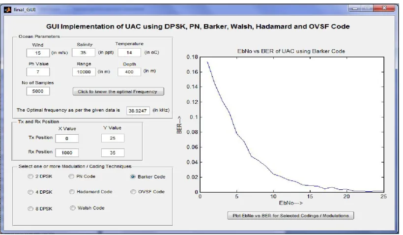
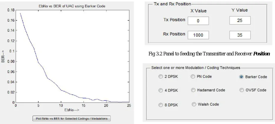
The GUI is designed into four section, in the first section as shown in figure1, the ocean parameters like wind speed, salinity, temperature, Ph value, Range (Distance between the transmitter and receiver), depth of the ocean are taken as input and according to the data, the optimal frequency will be calculated and shown in the Fig 3.1. In the second section, the transmitter and receiver position will be taken as the input and noise and attenuation will be calculated according to that data which is shown in Fig 3.2. The Fig 3.3 shows the third section in GUI design, in which we can select the type of modulation / coding techniques for which BER calculation will be displayed in Fig 3.4. The complete GUI is shown in Fig 3.5 which display the BER for UAC using

barker code where EbNo is ranging from 1 to 25. Fig 3.1 Ocean parameters to obtain the optimal frequency

Fig 3.2 Panel to feeding the Transmitter and Receiver Position

IV. CONCLUSION

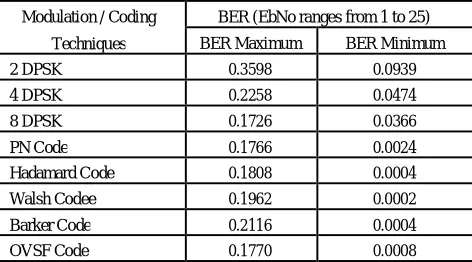
In our GUI model, we have considered all the necessary parameter and to model the channel, image mirror theory is used. Optimal frequency is calculated from the user data and the BER is calculated for the different modulation / coding techniques is shown in the Table 1. It is observed form the table that coding techniques gives better result than the DPSK. Using coding techniques we obtain the BER ranges from 0.2116 to 0.0002 (EbNo ranges from 1 to 25) which is 100 times better than 8 DPSK. To obtain the better

performance Orthogonal Frequency Division

Multiplexing (OFDM) and adaptive equalizer can be used. Equalizer will be effective in eliminating the ISI.

Table 1 : BER value for different type of modulation / coding Techniques

Modulation / Coding BER (EbNo ranges from 1 to 25)

Techniques BER Maximum BER Minimum

2 DPSK 0.3598 0.0939

4 DPSK 0.2258 0.0474

8 DPSK 0.1726 0.0366

PN Code 0.1766 0.0024

Hadamard Code 0.1808 0.0004

Walsh Codee 0.1962 0.0002

Barker Code 0.2116 0.0004

OVSF Code 0.1770 0.0008

REFERENCES

[1].Ruoyu Su, R. Venkatesan, and Cheng Li, A review of channel modeling techniques for underwater acoustic communications. PKP open coference

systems 2010.

[2].Camiel A. M, Van Moll, Michael A. et.al., A Simple and Accurate Formula for the Absorption of Sound in Seawater. IEEE Journal Of Oceanic

Engineering, 2009 : 34 : 4 : 610 – 616.

[3].Chengbing He, Jianguo Huang, and Zhi Ding. A Variable-Rate Spread-Spectrum System for Underwater Acoustic Communications. IEEE ournal Of

Oceanic Engineering, 2009 : 34 : 4 : 624 – 633.

[4].Abdollah Doosti Aref, Mohammad Javad Jannati, Vahid Tabataba Vakili. Design and Simulation of a Secure and Robust Underwater Acoustic

Communication System in the Persian Gulf. Communications and Networkv, 2011 : 3 : 99-112.

[5].Nejah Nasri, Abdennaceur Kachouri Laurent Andrieux et.al., Design Considerations For Wireless Underwater Communication Transceiver.

International Conference on Signals, Circuits and Systems, 2008 : 1 – 5.

[6].Nasri, N, Andrieux, L. ; Kachouri, A, et.al., Efficient encoding and decoding schemes for wireless underwater communication. 7th International

Multi-Conference on systems Systems Signals and Devices, 2010 : 1 – 6.

[7].Yang, T.C. Wen-Bin Yang. Low signal-to-noise-ratio underwater acoustic communications using direct-sequence spread-spectrum signals. OCEANS

2007 : 1 – 6.

[8].Jones A.D, Duncan A.J, Maggi A et.al. . Modelling acoustic reflection loss at the ocean surface for small angles of incidence. OCEANS 2010 :1 – 0.

[9].Guoqing Zhou and Taebo Shim. Simulation Analysis of High Speed Underwater Acoustic Communication Based on a Statistical Channel Model.

Congress on Image and Signal Processing 2008 : 5 : 512 – 517.

[10].ZHAO Yan-an ,ZHANG Xiao-min, HUANG Jian-guo,HE Ke. Simulations on Long Range Acoustic Transmission Characteristics Under Complex

Conditions. Second International Conference on Computer Modeling and Simulation 2010 : 309 – 313.

[11].Maria Palmese, Giacomo Bertolotto, Alessandro Pescetto et.al., . Spread Spectrum Modulation for Acoustic Communication in Shallow Water

Channel. OCEANS 2007 : 1 – 4.

[12].Ghada Zaïbi, Nejah Nasri, Abdennaceur Kachouri et.al., Survey Of Temperature Variation Effect On Underwater Acoustic Wireless Transmission.

5th International Conference: Sciences of Electronic, Technologies of Information and Telecommunications, 2009 : 1 – 6.

[13].Stojanovic, M. Preisig, J. Underwater acoustic communication channels: Propagation models and statistical characterization. IEEE Communications

Magazine, 2009 : 47 : 1 : 84 – 89.

[14].Nejah Nasri, Laurent Andrieux Abdennaceur Kachouri et.al., VHDL-AMS Modelling of Underwater Channel. Australian Journal of Basic and

Applied Sciences, 2009 : 3 : 4 : 3864 – 3875.