ABSTRACT
SIMOV, PETER RANGELOV. Investigating the Significance of “One-to-many” Mappings in Multiobjective Optimization. (Under the direction of Scott Michael Ferguson.)
Significant research has focused on multiobjective design optimization and negotiating trade-offs between conflicting objectives. Many times, this research has referred to the possibility of attaining similar performance from multiple, unique design combinations. These occurrences allow for greater design freedom. Their significance has not been used to quantify trade-off decisions made in the design space (DS). The current thesis computationally explores which regions of the performance space (PS) exhibit “one-to-many” mappings back to the DS, examines the behavior and validity of the corresponding regions associated with this mapping.
The research investigates the performances from two different sets of designs. One set contains Pareto-optimal designs, generated using multiobjective genetic algorithm. The second set of designs is generated using Latin Hypercube sampling over the design domain to obtain dominated performances. Mappings are generated from the PS of each set to the DS using indifference thresholds to effectively “discretize” both spaces. A mappings’s location in the PS and its mapped design bounds are analyzed. The total design hypervolume of the mappings contribute to design freedom.
The research investigates methods to support the decision-making of the designer in navigating designs once a performance region with high design freedom is chosen. The designs and their ranges are visualized to the designer in parallel coordinates. In complex situations designs, can span over large segments of the designs space and not exhibit distinct patterns. To address the complexity, designs are segmented into smaller relevant groups, whose mappings are validated.
To validate the mapping in a group of designs of selected performance regions, new designs are generated within the mapped design bounds. The fraction of designs that evaluate to the prior performance confirms the validity of the mapping.
Groups of designs are first selected by the application of a hierarchical clustering algorithm. Top-level groups have their mappings validated to support a selection of a group of designs. If the mapping information is deemed complex, the selected designs are further sub-divided using K-means clustering algorithm. The mapping information of each cluster of designs is validated. The process continues with a selection of a group of designs and applying hierarchical clustering again.
Investigating the Significance of “One-to-many” Mappings in Multiobjective Optimization
by
Peter Rangelov Simov
A thesis submitted to the Graduate Faculty of North Carolina State University
in partial fulfillment of the requirements for the Degree of
Master of Science
Aerospace Engineering
Raleigh, North Carolina 2010
APPROVED BY:
Andre Mazzoleni Gregory Buckner
Scott Ferguson Robert Nagel
DEDICATION
BIOGRAPHY
I was born in Bulgaria, finished high school in Vienna and graduated from Davidson College in North Carolina. I am a world traveler, who moved to Raleigh in 2008 to join the Mechanical and Aerospace Department at NC State University.
I valued the experience of living in this southern city for 2 years: a small laid-back city with tasty coffee.
ACKNOWLEDGEMENTS
I would like to acknowledge the tremendous support that I have received. My family has been very encouraging. I got into the habit of reading from my father, Rangel. I would attribute my affinity for numbers from my mother, Vasia. A conversation with my brother Kiril has always been able to put things in a better perspective.
I would like to thank the rest of the committee members. I appreciate the time and effort into shaping the thesis into a worthwhile effort, whose lessons will be valuable to me in the future. The support and council of my academic adviser, Dr. Ferguson, motivated me in pursuing the research efforts. His insights have helped me bring together my understanding of engineering and the ideas in this thesis.
I find the comments that Dr. Nagel, Dr. Buckner and Dr. Mazzoleni suggested to be very constructive. Their guidelines streamline the presentation within the thesis.
I have to note and thank contributions from my lab partners for suggesting revisions within the thesis: Callaway Turner, Garrett Foster, Micah Holland, Marc Tortorice, Ben
TABLE OF CONTENTS
LIST OF TABLES………. ix
LIST OF FIGURES………... xi
LIST OF USED TERMS………... xiv
1. An Introduction to Design Freedom and One-to-Many Mappings……… 1
1.1 Motivation for Design Freedom……….…3
1.2 Descriptions of performance-to-design space mapping ……… 5
1.3 Research Questions ………... 8
1.4 Outline of the Thesis……….. 11
2 Optimization and Research Background……… 12
2.1 Multi-objective Problem Optimization……….. 13
2.1.1 Use of MOGA Algorithms in Generating Solutions……….. 17
2.1.2 Design of Experiments Methods in Sampling………... 23
2.2 Analysis of Design Alternatives……… 24
2.2.1 Target Approximation……….………….. 25
2.2.2 Set-based design.……….…………..26
2.2.3 Target-seeking and Alternative Generation Algorithms………... 27
2.2.3.2 Parameterized Sets……….……….. 28
2.2.3.3 Inverse Design and Isoperformance ……….………..…. 28
2.2.3.4 Design Diversity in Evolutionary Algorithms ……… 29
2.2.4 Sensitivity Analysis..……….………. 31
2.3 Navigation in Design Space……….….. 32
2.3.1 Space Decomposition Research……… 32
2.3.2 Visualization Research……….………….35
2.4 Contribution to Quantifying Design Freedom ……….…………. 37
3 Research Approach……….……… 39
3.1Sampling the Design Space……… 41
3.2 Indifference thresholds discretization ……….……….. 49
3.3 Identify Mapping Type……….. 58
3.4 Rank Mapped Hypervolumes……… 62
3.5 Compare Performance of Mapped Hypervolumes……… 65
3.6 Visualization using Parallel Coordinates……….. 66
3.7 Cluster and group data……….………….. 71
3.8 Validate Mappings……….……… 75
3.9 Summary of Approach and Next Steps……….……… 82
3.9.1 Features addressed by the research approach..……….…….. 84
3.9.3 Look Ahead………... 87
4 Analysis of Case Study Optimization Problems………. 88
4.1 Analysis of Two Bar-Truss Problem………. 89
4.1.1 Sample Designs……….……… 90
4.1.2 Obtaining PS-to-DS data………….. 94
4.1.3 Ranking and Compare Sets ……….…………. 96
4.1.4 Design Navigation ………... 98
4.1.5 Impact of indifference thresholds ……….………… 111
4.2 Analysis of Vibrating Motor Platform Problem……….. 113
4.2.1 Sample Designs ……… 116
4.2.2 Obtaining PS-to-DS data ………….………….117
4.2.3 Ranking and Compare Sets ……….………. 119
4.2.4 Design Navigation ……….…….. 122
4.2.5 Impact of indifference thresholds ……… 132
4.3 Analysis of I-Beam Problem……….. 135
4.3.1 Sample Designs……….…… 136
4.3.2 Obtaining PS-to-DS data……….. 137
4.3.3 Ranking and Compare Sets ………. 139
4.3.4 Design Navigation ………... 142
4.4 Contributions to the Thesis ………... 151
5 Overview and Discussion………... 154
5.1 Revisiting the Research Questions……… 155
5.1.1 Research Answer of RQ1……….. 155
5.1.2 Research Answer of RQ2……….………. 157
5.1.3 Research Answer of RQ3……….………. 159
5.2 Sources for Future Studies………. 162
5.3 Limitations……….………… 163
5.4 Concluding Remarks………..…… 163
6 References……….……….…….…… 165
LIST OF TABLES
Table 3.1. Results from performance space discretization……… 57
Table 3.2. Results from design space discretization……….……. 58
Table 3.3. Quantification of mapping types……….……. 61
Table 3.4. Cluster Analysis using Mapping Quality Information……….……… 81
Table 4.1. List of tested problems……….………. 88
Table 4.2. Results from performance space discretization……… 94
Table 4.3. Results from design space discretization……….……. 95
Table 4.4. Quantification of mapping types……….. 96
Table 4.5. Top Hierarchical Clusters Analysis on top branches……… 103
Table 4.6. Centers of Top Hierarchical Cluster Analysis……….………. 103
Table 4.7. 4 K-Means Cluster Analysis ………..……….…………. 104
Table 4.8. Centers of 4 K-Means Cluster Analysis………... 105
Table 4.9. 5 K-Means Cluster Analysis………. 105
Table 4.10. Center of 5 k-Means Clusters Analysis……….. 106
Table 4.11. Top Hierarchical Clusters Analysis on top 4 branches……….….. 107
Table 4.12. Centers of Top Hierarchical Clusters ……….……… 108
Table 4.13. Indifference threshold discretization……….. 111
Table 4.14. Design discretization analysis……… 112
Table 4.16. Results from performance space discretization……….……. 118
Table 4.17. Results from 5% design space discretization………..…… 118
Table 4.18. Quantification of mapping types………. 119
Table 4.19. Top Hierarchical Clusters Analysis……… 124
Table 4.20. centers of Top Hierarchical Clusters Analysis………...…… 125
Table 4.21. 4 K-means analysis. Design variables associated with yellow branch……...… 131
Table 4.22. Discretized design variable ranges……….… 133
Table 4.23. Mapped ranges for designs of (-522, 231) PSB………..… 134
Table 4.24. Design discretization analysis………. 134
Table 4.25. Results from performance space discretization……….. 138
Table 4.26. Results from design space discretization……… 139
Table 4.27. Quantification of mapping types……….… 140
Table 4.28. Top Hierarchical Clusters Analysis……… 144
Table 4.29. Centers of Top Hierarchical Clusters Analysis………..……….…… 145
Table 4.30. 5 K-means clustering……….. 146
Table 4.31. Cluster Centers in 5 K-means clustering………..……….. 147
Table 4.32. 10 K-means clustering……… 147
Table 4.33. Cluster Centers in 5 K-means clustering……….……….….. 148
Table 4.34. Top Hierarchical Clusters Analysis……… 149
Table 4.35. Mapped Design Hyperbox Bounds Ranges……… 150
LIST OF FIGURES
Figure 1.1. Mapping between design and performance spaces ……… 6
Figure 1.2. Quantifying the mapped region in the design space ……….. 7
Figure 2.1. Pareto-optimal front for 2 objective function ……… 16
Figure 3.1. Research approach ………. 39
Figure 3.2. Feasible Performances of LH Sampling……….. 45
Figure 3.3. Latin Hypercube Sample of designs……….. 46
Figure 3.4. Pareto-optimal performances for the two objectives……….. 47
Figure 3.5. Design space for the Pareto-optimal designs……….. 48
Figure 3.6. Pareto and LHS Performances of the studied function……….. 48
Figure 3.7. Performance space box boundaries defining a target performance……… 50
Figure. 3.8. Discretized performances of LHS…...………... 54
Figure. 3.9. Discretized performances of Pareto set...………... 55
Figure. 3.10. Discretized LHS designs…...………... 55
Figure. 3.11. Discretized designs of Pareto set……….. 56
Figure. 3.12. An example of a one-to-one mapping………... 59
Figure.3.13. An example of a one-to-many mapping……… 59
Figure 3.14. Design MEHV for Pareto-optimal and LHS sets……….. 64
Figure 3.15. Average-weighted Performance space location of 6 large MEHVs…………. 66
Figure 3.17. Mapped 2-D design space of the selected PSB……… 69
Figure 3.18. Parallel Coordinates of the selected PSB..……… 70
Figure 3.19. Sample designs………. 73
Figure 3.20. Sample dendrogram……… 73
Figure 3.21. Branch division in similarity………. 74
Figure 3.22. Navigational process diagram……….………. 78
Figure 3.23. Hierarchical cluster analysis on the data……….………. 79
Figure 3.24. Validate Mappings ……….………. 80
Figure 3.25. K-means application on 4 designs……….…… 82
Figure 4.1. A visualization of a 2 bar-truss problem………. 89
Figure 4.2. Performances on the Pareto-optimal front and LHS designs………. 94
Figure 4.3. Pareto-optimal designs……….….. 95
Figure 4.4. Design LH sampled designs……….…….. 96
Figure 4.5. Design MEHV for Pareto-optimal and LHS sets……… 97
Figure 4.6. Performance space location of large MEHVs………. 97
Figure 4.7. Performances associated with selected PSB………... 99
Figure 4.8. Parallel Coordinates representation of mapped designs………. 100
Figure 4.9. Hierarchical Clustering, top 3 branches……….. 102
Figure 4.10. Second level hierarchical analysis on designs. Top 4 branches shown……… 107
Figure 4.11. Second level hierarchical analysis on designs……….. 109
Figure 4.13. Sum of MEHV for Two-Bar Truss……… 113
Figure 4.14. Platform for a Vibrating Motor………. 114
Figure 4.15. Pareto-optimal front and LHS Mapped Performance sets……… 117
Figure 4.16. Design MEHV for Pareto-optimal and LHS sets……….. 120
Figure 4.17. Performance space location of large MEHVs………... 121
Figure 4.18. Performances within the selected Performance Space Region………. 122
Figure 4.19. Parallel Coordinates representation of mapped designs……… 123
Figure 4.20. Hierarchical Clustering on top 5 clusters……….. 124
Figure 4.21a-e. Validation procedure. Performances in proximity to the PSB………. 126
Figure 4.22a-e. Validation procedure in Performance Space……….... 128
Figure 4.23. Sum of MEHVs……… 134
Figure 4.24a. Side view of an I-Beam……….. 135
Figure 4.24b. Cross-sectional view, showing the four variables……….……….. 135
Figure 4.25. Performance space of Pareto set and selected LHS sampling………... 137
Figure 4.26. Design space mapped volume for LHS and the Pareto sets ……… 140
Figure 4.27. Performance space location of large MEHVs……….. 141
Figure 4.28. Selected PSB……… 142
Figure 4.29. Mapped Designs of Selected PSB……… 143
Figure 4.30. Hierarchical clustering with top 7 branches colored……… 144
Figure 4.31. Hierarchical Clustering on 12 designs, cluster id8……….. 149
Figure 4.32. Designs in the red branch of the hierarchical analysis……….. 150
LIST OF USED TERMS
Design: a design configuration described in m real-valued components, 𝑥⃑𝜖ℝ𝑚.
Design Performance: the performance of a design evaluated in n objectives, 𝑓⃑𝜖ℝ𝑛.
Indifference threshold: a variable threshold within which designs are equivalent to each other.
Performance Space Box (PSB): a performance region, 𝑏
𝑓⃑𝑗., characterized by indifference
thresholds. It contains a set of equivalent performances.
Design Space Box (DSB): a design region, 𝑏𝑥⃑𝑖. , characterized by indifference thresholds, It contains a set of equivalent design configurations.
Mapped Designs: design configurations that belong to one PSB.
Mapped Design Range: the variable range of mapped designs, that evaluate to a PSB.
1. An Introduction to Design Freedom and One-to-Many Mappings
“The intent of analysis is to design; without design intent the analysis would seem to have no purpose. […] “Design intent builds intelligence into the analysis.”
- Panos Y. Papalambros, JMD editor (Papalambros, 2010)
The design of engineering systems becomes an elaborate and demanding process. Engineers are expected to tackle complex tasks in a structured and efficient manner. Design research provides assistance to engineering decisions through an analysis of the attributes and corresponding functions of studied systems.
What constitutes design? Papalambros‘s quote has that the ―intent‖ of the analysis is what constitutes ―design.‖ The assistance the design process provides is the incorporation of ―intelligence‖. The study of design engineering creates value in engineered systems.
The goals of an engineered system vary according to what a consumer seeks and the environment in which it is anticipated to operate The functionality of a system is assumed to be measurable through some metric. As a result, designers can evaluate the performance of multiple designs through the configured system attributes.
obvious and physically relevant example can be given in designing yogurt cups or soda cans that contain a specified amount of substance but differ in their physical configuration. Complex engineering systems, such as in the automotive industry, can also exhibit cases where reaching a goal is possible through multiple designs. This thesis addresses such situations in engineering design. This is stated through the following definition, which is used within the current thesis:
Definition: Design freedom associates unique performances that are reached by multiple
and dissimilar design configurations
The definition leaves the designer to choose a metric to measure dissimilarity of design configurations. It can be noted that the given definition is associated and tied to some specified performance. The definition does not reflect the effects that design variations exhibit on the system. It contrasts with the definition for design freedom given in (Mistree, 1998), which refers to ―design freedom as the extent to which a system can be "adjusted" while still meeting its design requirements‖. Mistree‘s definition is based off a particular design, whose configuration is ―adjusted‖. In this work, the differences between unique designs with similar performance are the deciding factor in establishing design freedom.
one-to-many mappings. The research questions that drive this work are discussed in Section 1.3. The steps that are taken in the development of the thesis are described in Section 1.4.
1.1 Motivation for Design Freedom
Suppose that there is a case when multiple and dissimilar designs evaluate to the same performance. This presents design freedom to the designer. The availability of choices between alternative design configurations supports the analysis of systems beyond their performance.
Considerable research has focused on multiobjective design optimization and negotiating trade-offs between conflicting objectives (Kasprzak, 2001, Tappeta, 1997, Mattson, 2004, Wu, 2001, Marler, 2004). Many times, research in this area has referred to the theoretical possibility of attaining similar performances from multiple, unique design combinations (Chen, 2008), studied under topics such as ‗design flexibility.‘
allow consumers to specify products with similar functionality, yet unique form. Now, imagine a scenario where customers can define their functional specifications, and are then presented with corresponding design space information. In cases where a performance space location maps to a single location in the design space, the customer has limited design freedom in terms of style and fit and comfort. Conversely, if a single performance space location maps to multiple, diverse locations in the design space then the customer has increased design freedom with which to ―personalize‖ the product.
Accommodating a set of alternatives in the design space creates the possibility of considering trade-offs in the configuration choice. Discovering alternatives can create a wide selection of choices to allow decisions to be taken not only with respect to the computed performance but also according to the strength of preferences to design configurations. The benefits of establishing design freedom are the ability to alternate between dissimilar designs throughout the design process.
Such one-to-many mappings between the performance and design space have been previously hypothesized to yield increased design freedom (Ferguson, 2005ab). They are introduced in Section 1.2.
1.2 Describing performance-to-design space mapping
This section describes how designs are located in performance space. Given a design variable vector , and objective functions , this design evaluates to a multidimensional performance value .
Engineers work in the design space (DS) by selecting designs . This is where the designer establishes the settings of the system: establishing geometric shape, adding or removing modules, defining possible platforms, and receiving variable values from other designers. Each point in the design space is equivalent to a unique design. The performance space (PS), represented by the functions F1through Fn, specifies the value of a design with respect to each objective.
Unlike design-to-performance evaluation, which is a one-to-one mapping, performance-to-design space mappings do not necessarily have a singular mapping. Instead, the possibility exists that a single point in the performance space maps to multiple points in the design space. Under this notion multiple designs yield the same performance. Consider this analogy: when designing an automobile, the fuel economy of the vehicle can be uniquely determined when the powertrain and various geometric dimensions of the vehicle are specified. However, given a desired fuel economy, there may be many vehicle configurations capable of achieving the target. The concepts of one-to-one and one-to-many mappings are illustrated in Figure 1.1.
Figure 1.1. Mapping between design and performance spaces
one-to-one and one-to-many mappings. For a one-to-one mapping, designs come from similar or identical designs. Conversely, for one-to-many mappings, designs come from dissimilar or distinctive designs. The deciding factor is an indifference threshold chosen as appropriate by the designer. The process allows the designer to consider the bounds of the mapped region in making informed decisions. These bounds are shown in Figure 1.2.
Figure 1.2. Quantifying the mapped region in the design space
1.3 Research Questions
The analysis of product variations is a valuable part in the consideration of designs (Olewnik, 2005). Efforts have been pursued by several authors to investigate this possibility (Chu, 2010, Malak, 2008, Hohm, 2009, Preuss, 2006, Ferguson, 2005ab, Gupta, 2006, de Weck, 2006, Messac, 2000). The current thesis uses the following research assertion in using one-to-many mappings to quantify design freedom:
Research Assertion. One-to-many mappings exist and identifying them signifies value in
attaining design freedom
The thesis demonstrates the existence of one-to-many mappings in presenting numerical case study problems. The methodology in applying one-to-many mappings is developed. The value of one-to-many mappings in quantifying design freedom is consecutively established.
Research Question 1: Do one-to-many mappings located on the Pareto frontier show significantly less design freedom than those in sub-optimal regions?
This research question requires the comparison of one-to-many mappings located both on the Pareto frontier, which contains the multiobjective optimal designs, and sub-optimal regions. Answering this question will provide insight into whether choosing sub-optimal performances leads to higher design freedom while identifying the necessary performance tradeoffs.
Computational parameters within the research approach can affect the identification of a subset of one-to-many mapping occurrences. The effect of these parameters must be discussed, and the importance evaluated, when identifying design freedom. Of particular interest is the selection of indifference threshold values, which discretize design parameter values. The second research question is posed to address the use of indifference thresholds given an identified performance mapping:
Research Question 2: How is the sensitivity of design freedom with respect to indifference thresholds characterized?
Definition: Mapping Quality (MQ) signifies the extent that designs within an identified
region of the design space maps to the original target performance space region
In Fig. 1.2, the reader can note that the area between the mapped designs has ‗gaps‘ of sampled designs in between. The designs that exist in the region between those designs may not be associated with the targeted performance. In effect, MQ addresses the effectiveness of the mapping procedures given a particular set of designs. This leads to the third research question:
Research Question 3: Research Question 3: Can methods be implemented to explore design choices, in order to identify mapping trends and visualize the data?
1.4 Outline of the Thesis
The section examines the direction that the thesis will take and procedure steps that will be taken in answering the research questions. Section 1.1 established that there is a demand to categorize design freedom. This is required in order to achieve a greater competitive advantage through the inclusion of design variability. Section 1.2 showed the mapping relationship between performance and design space regions when identifying design freedom.
2. Optimization and Research Background
“There is nothing like looking, if you want to find something. You certainly usually find
something, if you look, but it is not always quite the something you were after.‖
- J.R.R. Tolkien, The Lord of the Rings
Engineering design employs a variety of techniques to analyze, study, and assist the decision-making processes. This chapter visits prior research efforts that cover design optimization, design of experiments, sensitivity analysis, tradespace navigation strategies and visualization techniques. These prior research efforts form a basis into quantifying design freedom.
Three research questions were posed in Chapter 1. The questions are inspired from the possibility of analyzing design freedom. Research Question 1 seeks to determine and compare design freedom between Pareto-optimal and suboptimal regions of the space. Research Question 2 addresses the methodology of the computational process, in particular, what are the effects of varying indifference threshold size. Research Question 3 addresses the tools and visualization that support the decision-making process.
review identifies that researchers have been interested in studying design freedom and the generation of design alternatives. However, performance-based approaches have been overlooked as a suitable tool in determining design freedom. This finding signifies a current opportunity to employ one-to-many mappings as a performance-based method toward the quantification of design freedom.
The chapter is split into three major sections. Multiobjective problem optimization is discussed in Section 2.1. Prior research associated with the topic of design freedom is presented in Section 2.2. Design navigational tools and visualization methods are placed in Section 2.3. The design optimization strategies usually involve complex systems with multiple parameters and objective functions. The next section presents background of optimizing engineering systems.
2.1 Multiobjective Problem Optimization
Computational developments provide the necessary means to evaluate large-scale complex engineered systems (Eddy, 2002). This increased problem complexity typically requires that multiple attributes and decision criteria be considered when choosing a design configuration. This yields multiobjective problems with often expensive black-box evaluation costs (Shan, 2010, Lee, 2009, Jones, 1998).
Designs variables represent the attributes, i.e. inputs, of the system being studied. This thesis assumes that the design variables can be represented as real-valued vectors. Thus, a vector representing m system attributes is s.t. . Each performance characteristic is represented as an objective function. Evaluating through functions , where n is the number of characteristic performances, yields system performance. In the current thesis, we assume that the objective functions are real-valued and the performances can be presented as
.
The standard form of an optimization problem requires that we minimize all objective functions while comparing possible trade-offs between the n performances (Vanderplaats, 2007, Kim, 2006). The form also includes inequality and equality constraints, and respectively. These constraints define unfeasible regions of the design space in which no possible solution exists. The formal optimization problem statement is given by Equation 2.1:
s.t.
Where
Optimality is not restricted to a singular point due to the possible trade-offs across performances. The considerations of trade-offs is important for multiobjective problems in which it becomes an inherent feature. Trade-offs occur when objectives start to compete with each other. It is common that a particular performance component can be improved only by sacrificing an improvement in another one. The solution then becomes a set of optimal points for the combination of performance objectives (Vanderplaats, 2007, Pareto, 1906). The set of optimal points is called the Pareto-optimal set. A Pareto set consisting of performances P1, P2
and P3 on Pareto front is shown for a generic 2 design variable, 2 objectives problem in Figure
2.1. The performance point P1 performs well in F1 and poorly in F2. Conversely, P3 performs
well in F1 and poorly in F2. The performance of P2 presents a possible trade-off between the two
Figure 2.1. Pareto-optimal front for 2 objective function
However, some problems can contain Pareto sets that map to few selected regions in the design space. As such, there can be regions in the design space that correspond to optimality (Preuss, 2007, Shan, 2010). The Pareto frontier or some sub-part of it can have analytical solutions. Thus, it is possible that some mapped optimal designs can be fit into analytical solutions or some pattern.
There are multiple issues to consider in optimizing a problem. A way of converging to the set of optimal solutions has to be found, while constraint violations yield infeasible designs. Therefore, the design sampling has to be chosen in an effective manner. The following section covers computational techniques in optimizing multiobjective engineering problems designs.
2.1.1 MOGA Algorithms in Generating Solutions
This section presents methods that seek optimal solutions in multiobjective optimization problems. A method called Non-Dominated Sorting Algorithm-2 (NSGA-2), an implementation of a multiobjective genetic algorithm (MOGA), is discussed in additional detail. The NSGA-2 algorithm is employed in the research approach and is described in Chapter 3.
be devised from the standard problem definition in (2.1) that assigns different weights to each performance to combine the problem as a single-objective problem optimization. That is an example of a weighted sum method (Vanderplaats, 2007). Challenges in applying a weighted sum approach include expanding its performance to non-linear problems, spread of the derived Pareto set, and computational time in deriving the whole Pareto front. Some other search techniques are linear programming or stochastic methods such as simulated annealing (Vanderplaats, 2007, Park, 2007), goal programming algorithms (Deb, 2001), physical programming (Messac, 2000), or Compromise Decision Support Problem (Mistree, 1995). Determining and including the robustness of solutions into the optimization has also been undertaken as a research direction (Li, 2006, Azarm 2006, 2009).
It is important to obtain a representative and high-quality Pareto set. Otherwise, challenges may arise in the consequent steps of the design process. Discussions on the quality of different Pareto sets can be obtained in (Deb, 2000, Azarm, 2001, Marin 2009). The metrics that they introduce focus on finding an accurate and close representation across the whole Pareto frontier. Some of the metrics (Azarm, 2001) involve representing the Pareto front as widely as possible without having overlapping performances that would lower the informational content of the Pareto set.
run and are applicable when dealing with continuous and discrete variables. MOGAs can also be extended to optimization problems with hierarchical structure as well (Kaufmann, 2010).
A distinguishable feature of MOGAs is that they are evolutionary population-based strategies. The search is performed using a population of designs. Once the population of designs is evaluated, a new generation of designs is created for the next iteration. Since there are multiple designs, the population, as a whole, is able to sample and explore large sections of the design space. This is particularly useful in complex multidimensional problems. In later iterations, MOGAs exploit the most promising design regions for optimality and converge onto a solution.
Genetic algorithms refer to design variables as ‗genotypes‘ and the performance as ‗phenotypes‘. These names stem from the origin of genetic algorithms. They were modeled after genetic recombination (Ebernhart, 2001) and try to mimic the biological adaptation in an optimization setting (Deb, 2001). The fitness, i.e. goodness, of a design is defined by its phenotype. The genotype includes the encoding of a particular individual (i.e. design).
The population of individuals has to be initialized. This can be done through heuristic measures or a database of previously computed designs. A randomly-generated population can also be used, and once initialized, the MOGA enters a process of iterative adaptation in the search for optimality defined by fitness.
in both algorithm architecture and in its resulting performance. There are three common steps among GAs:
Selection: the choice of which designs to base next generation on. Some of the designs, usually the more optimal ones, are used in generating the next-turn‘s population.
Crossover: in creating the next generation, the genotype of the new designs has to be chosen. The information of the designs that passed the selection phase is used. This ensures that the high-performing genotypes remain within the population. The crossover stage exchanges variable information between designs.
Mutation: the step randomizes an individual‘s phenotype. This ensures variations are introduced into the population. This process allows for exploration of unsampled regions of the space.
After the designs have been selected, their genotype is crossed between two parents and a number of offspring. This allows a population of designs that sample the design space to search for both local and global minima. Here the phenotype drives the fitness and the search is performed by changing the genotype.
stochastic elements and this makes their analysis dependant on numerical runs. Therefore, it has been suggested to run an optimization more than once to ensure that the optimal solution has been obtained (Vanderplaats, 2009).
The type of algorithm and implementation clearly affects the optimization process. Among the algorithms, and of particular interest, is the Non-dominated Sorting Genetic Algorithm-2 (NSGA-2), as shown in (Deb, 2000, Deb, 2001, Deb, 2002). The differences between NSGA-2 and other MOGAs include methods of working with dominated solutions and consequent crossover between solutions. NSGA-2 preserves a number of individuals with the highest fitness onto the next iterations, making it an elitist MOGA. It uses sorting to compare performances between multiple dimensions of the individuals in the population. Its complexity in sorting through the solutions is given as ( ), where n is the number of objectives and z is the size of the population (Deb, 2002). Furthermore, it also includes niching techniques that preserve design diversity (ibid).
space and to seek solutions that can yield better optimal values. The process is aimed at avoiding local minima (Deb, 2001). Given a region of interest, the ‗exploitation‘ stage finds and converges onto the best solution within the region. While the size of the population clearly affects these processes, no clear-cut boundaries are established due to the stochastic aspect of optimization (Deb, 2001). The diversity of the population is important, especially in the ‗exploration‘ aspect of the optimization process.
Goldberg and Deb show the use of diversity in developing genetic algorithms and techniques. (Goldberg, 1989). They developed the use of ‗niching‘ techniques that use measures of the spread of solutions in either phenotype (performance) or genotype (design space). The step measures distances between points in the population sets in either one of the spaces achieving a high coverage of solutions with the goal of avoiding similar designs.
There are three main reasons to select the NSGA-2 algorithm: 1) the code is robust and easily configurable to a variety of engineering problems; 2) the algorithm was shown to generally outperform other MOGA algorithms (Strenth Pareto Evolutionary Appoach -1 (SPEA-1), Vector Evaluated Genetic Algorith (VEGA) and NSGA-1, (Deb, 2001)); and 3) the algorithm has been introduced as part of available software packages.
populations, which can capture the Pareto frontier very closely. The code is, therefore, implemented in the research approach in finding the Pareto set. This is presented in Chapter 3.
2.1.2 Design of Experiments Methods in Sampling
Design of Experiments (DoE) refers to methods that generate suggested designs in the sampling of a problem. They can be used in determining function‘s behavior and identifying influential variables in an effective manner. The most basic sampling technique is probably grid sampling or grid search (Vanderplaats, 2007). Along a given dimension, it places test designs a uniform distance from each other. As a number of designs are evaluated, it can exhaustively test a problem. The method is not advised as an efficient manner to test black-box problems. Large regions of the space need not contain any additional information concerning the problem, as they can be associated with less sensitive or non-influential variables. Therefore, for computationally expensive problems, sampling a grid can become time prohibitive for an effective search. Different strategies have been devised to avoid this problem.
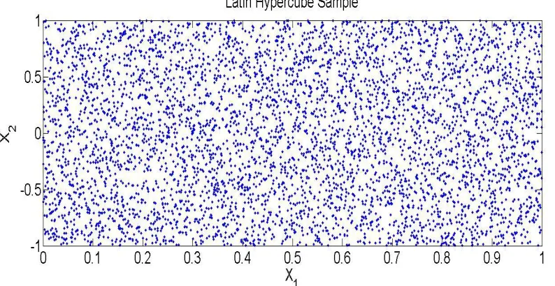
One possible choice is the use of Latin Hypercube Sampling (LHS), which has been investigated in engineering design successfully (Chen, 2009). Here, an individual variable can be stratified, or split, into different test intervals. This creates a series of non-overlapping regions that represent the domain in a uniform fashion and is suitable for test sampling. LHS design uses such intervals as one of its main features, in that it splits the domain of each dimension of a multivariable problem into the same number of intervals, s. Within a given interval, chosen for sampling, the method assigns a design through some calculation. For example, thr lhsdesign function in Matlab uses randomly generated designs within each interval as its default setting. A key feature of a definition of a LHS design is that the test designs are chosen to sample any direction of the domain the same number of times. For a 2 dimensional grid, this forms a Latin Square – hence the name, Latin Hypercube Sampling. Such a sampling technique reduces the uncertainty in the obtained performance compared to a generalized randomized sampling. These features make it a common sampling procedure and it is incorporated in the research approach.
2.2 Analysis of Design Alternatives
in. This section will cover several topics in design variations and alternatives. Presented topics are listed below:
Target approximation through Design of Experiments Set-based design
Target-Seeking and alternatives generation Sensitivity and robust analysis
2.2.1 Target Approximation
Performance regions have had to be approximated and analyzed for a variety of reasons. In reliability analysis (Bertsche, 2009), regions that lead to failure are avoided. The performance space, therefore, has to be characterized with particular attention to the boundaries between regions that have to be avoided and those that have to be optimized (Picheny, 2010, Ranjan, 2008).
2.2.2 Set-based design
Set-based design approaches (Finch, 1997, Chen, 1999, Chen, 2008a, Shan, 2004, Sobek, 1999) have been used in concurrent engineering environments as a means of maintaining opportunities to change designs at a later stage. In comparison to the definition given in Chapter 1, this quality is also sometimes referred to as design freedom (Chen, 2008a).
Set-based design involves making decisions between sets of possible designs. It therefore maps a region of design space to a region of the performance space. Through the design process, the decisions are adapted and a single design is chosen as information about the system accumulates. Motivation for this approach is to delay the need for making design commitments until later in the design process.
Recent work (Madhavan, 2008) has shown that in an industrial setting, set-based design approaches reduce the number of iterations between design teams and provide a library of back-up design options. Research in target sets to decompose the design space and identify optimal solutions was conducted in (Chen, 2008a). Physical Programming methods developed in (Chen, 2000, Messac, 2002) differentiate solutions into five different types based on the quality of the solution, considering all solutions within the same type equivalent.
of design freedom. The analysis of design freedom can be adjusted to yield sets of possible options within some measure of equivalency, making it similar to Physical Programming.
2.2.3 Target-seeking and Alternative Generation Algorithms
This section introduces target-seeking algorithms and techniques that seek alternatives in the design space. A common method to find unique solutions with a similar performance is through a two-level optimization. The first run determines the performances that are optimal or functional. The second run of the optimization contains the objective to minimize the deviation in performance while maximizing the distance between designs. Such approaches are commonly referred to as target-seeking or goal-seeking algorithms.
2.2.3.1Modeling to Generate Alternatives
space around the optimal value but within which performances are acceptable. This can be envisioned by building a ‗box‘ around the targeted region.
2.2.3.2Parameterized Sets
The search for alternatives in decisions trees has been recently pursued by Paredis and Malak. The design freedom framework as defined in (Malak, 2008a) and (Malak, 2009) is based on a tree of decisions that design engineers take in the process of product development. Design freedom becomes the ability to reach appropriate performances by backtracking on the decisions leaves. The approach has potential to grow into a more extensive framework for exploring and characterizing engineering decisions. One aspect of their research is the use of support vector machines (SVM) in identifying domain regions which can be extended to other predictive engineering environments. Nevertheless, the authors work outside the design space. This impedes its integration for functional analysis of design freedom.
2.2.3.3Inverse Design and Isoperformance
De Weck (2004) has introduced the notion of isoperformance, in which a formulation for efficient level sets of designs with similar performance is presented. This work uses the Jacobian of the inverse matrix to generate the contours. These are then used to evaluate the design concepts, while also evaluating the constraint restrictions. A possible practical issue is that black-box problems might not have easily accessible Jacobians.
2.2.3.4Design Diversity in Evolutionary Algorithms.
The current section reviews the process of using design diversity in computational frameworks of evolutionary algorithms (EA). MOGA belong to EA and they are introduced in the earlier section 2.1.1. Different EA, and in particular MOGAs, employ design diversity, a measure of variations that exist in a given design population, in the process of solving for optimal solutions.
The use of diversity in computational frameworks creates an analogy for design freedom in a computational setting. It has shown benefits in the optimization process (Deb, 2001, Vanderstaal, 2008, Ehrgott, 2009). Sampling the space, while preserving design diversity, is a computationally efficient method to explore the design space. It presents the potential that the use of diverse sets of solutions is able to achieve.
Diversity-seeking algorithms have a potential in generating solutions with high level of design freedom.
A method is presented in Hacker (Hacker, 2001) which aims to determine the modality of a problem. The research changes the exploitation stage of the optimization. This approach computes the variance of the population in both performance and design space. This information is used to choose a strategy for exploitation of a performance space at any given stage of the optimization. It is an example of using a diversity-dependant strategy in improving the optimization process.
An earlier work, (Bennini, 2003) treats diversity as an individual objective to steer the population to higher design freedom. The method involves assigning a diversity measure to the individuals in the population and using it in the selection stage of the algorithm. The effect is to assign an additional fitness measure.
2.2.4 Sensitivity Analysis
This section covers applied and analytical methods into robustness and sensitivity analysis. The goal of these approaches is to characterize the effects that design variables changes have on performance. Robust design is aimed at reducing performance changes due to uncontrollable variations of a design. Sensitivity analysis is a field of study that aims to identify contributing factors into performance variation through a far-reaching statistical and scientific background (Cacucci, 2003, Saltelli, 2008, Giassi, 2004, Goh, 2007, Turner, 2007, Yin, 2008). It uses DoE sampling to test problems and characterizes the variations in performance to identify the most influential parameters given a particular effect. In (Saltelli, 2008), a study is performed on a batch reactor to identify when a thermal runaway occurs. It is an undesirable event to be avoided in practical applications. The study extends to determine which factors contribute to minimize the possibility of this event through regression models. Robust design, on the other hand, can improve reliability in applied engineering systems (Azarm, 2005).
Even though these aforementioned methods have a wide use, the authors have not encountered a sensitivity analysis aimed at design freedom originating with performance values.
2.3 Navigation in Design Space
Sampling designs and optimizing the solutions can lead to a large amount of information regarding the solutions. The decisions that designers have to make become a demanding task for complex engineering systems. This is due to the high number of decision variables and problem complexity. The abundance of information can create a bottleneck for the designer by obstructing some of the underlying structure. For example, a human can usually rationally consider up to 7 pieces of information at once (Eysenck, 2005).
This section deals with existing issues of navigating the design space. The section is split in two sub-sections: investigating structural information through decomposition techniques; and visualization techniques used in design research.
2.3.1 Space Decomposition Research
space decomposition techniques that classify or group parameters of designs. The current section investigates what methods exist to relate the performance-to-design spaces and whether they can be applied to address RQ1 and RQ3. The methods presented herein include K-means clustering, hierarchical clustering, artificial neural networks and support vector machines.
An important research direction, listed in (Shan, 2010), is the ability to differentiate design regions with respect to their potential performance values. Optimal regions are commonly confined within a small area of the design space. Identifying the useful regions in a problem could increase the effectiveness of search algorithms. Furthermore, optimization strategies can potentially benefit from classification techniques through the use of correlation among parameters.
An option of partitioning the design space is using rough sets theory. Rough sets apply thresholds in decomposing the design spaces. The partitioning is assigned according to performances from designs of the associated regions. The final result maps target performance to associated design regions. The research is shown in (Chu, 2010, Chen, 2007, Shan, 2004). The process is aimed at multidisciplinary complex designs.
in a dendrogram. Here, the leaves are the final designs and intermediate branches signify common features among the dataset of designs.
In hierarchical clustering, similarity between designs, or a group of designs, is first computed (Karypis, 2004). The information generates a similarity matrix that contains distances between designs. Starting from individual designs, which form the leaves of the dendrogram, the data is then repetitively merged into larger groups. A larger group corresponds to a higher level in the branch tree. For a binary tree, the data is combined to a single branch.
One method to unite groups of designs together is to evaluate the shortest distance between elements of each two branches. The metric is called ‗single‘ within Matlab. A node is then constructed by merging the branches that are closest to each other. In the unweighted average distance (UPMGA) metric, the distance between every member that belongs to two different branches of a tree is computed to evaluate the distance between these two branches. The two branches with the smallest distance are then united in a branch of one level higher. Clusters can then be further derived on the ending branches of the tree that form groups.
centers are updated in consecutive iterations. The objective is to minimize the total distance from within the designs to their assigned cluster centers and maximize the distance between clusters. The metric to measure distances is chosen by the user. The algorithm is stochastic, whereby a single run might be stuck in local minima. It is suggested that multiple runs are performed to confirm the cluster distribution. In searching for a balanced representation, it is also advisable to have multiple runs with different number of clusters.
2.3.2 Visualization Research
This section introduces current visualization tools that are used to represent the complex information associated with a design‘s configuration. Several approaches have been developed that communicate the data related to a problem, which include solutions and allow for interaction with the human decision-maker (Eddy and Lewis, 2002, Frecker, 2009, Naone, 2010, Shneiderman, 2006, 2007, Wolf, 2009). Scientific and information fields use visualization to exchange complex information (Wolf, 2009) and visualization procedures are undergoing further research development.
multidimensional scatter plots, network graphs and textual analysis. These methods can be used to relay complex information interactively to a user.
The requirements for design visualization suggest the use of interactive methods in an engineering environment. Frecker and Finger present (Frecker, 2009, Frecker. 2009) the use of DesignWeb, an interactive navigational design toolbox. Their research uses it for the summarization of knowledge, reuse and analysis of designs. One of its capabilities is creating a graph representation of core concepts and generating relationships between them using textual analysis and clustering algorithms.
Visualization systems have to allow for the analysis of performance attributes while navigating the design space. A ‗Design by Shopping‘ approach (Wolf, 2009; Eddy, 2002) samples the design space and then allows designers to pick regions they want to explore further. Another type of design visualization is explored through the Applied Research Laboratory Trade Space Visualizer (Wolf, 2009, Simpson, 2004, 2008). Simpson et al. studied representation of MultiDimensional and MultiScale Interactions and used ATSV to navigate through a complex interacting design space. It is capable of visualizing multidimensional data by plotting all of the designs. This process fosters the identification of major trends in the data visually, such as the existence of clusters of data.
visualization techniques in addressing RQ3, namely parallel coordinates, in conjunction with space decomposition to ease the navigation in design space for the user.
2.4 Contribution to Quantifying Design Freedom
The aforementioned methods cover a variety of topics that become important as enabling technologies in examining design freedom. The current section is a convenient place to review the steps that have been taken and map the next steps. Points that have been raised in this chapter are the following:
Pareto optimality and performance trade-offs
Multiobjective Genetic Algorithms as an optimization tool Latin Hypercube Sampling as Design-of-Experiments
Methods analyzing or seeking variability (sensitivity analysis, target-seeking algorithms)
Space decomposition (K-means and hierarchical clustering, SVM) Visualization methods
identify the Pareto front effectively, while LHS samples the design space to yield an informative representation of the associated performance space. Displaying the solutions allows decisions to be made effectively. Nevertheless, conveying the data for highly dimensional problems becomes a hard issue itself. Clustering can capture the information of the mapped designs to identify principal properties. The information is given this information in taking decisions more effectively.
3. Research Approach
“Begin at the beginning and go on till you come to the end: then stop.”
The King, In “Alice in Wonderland”, Lewis Caroll
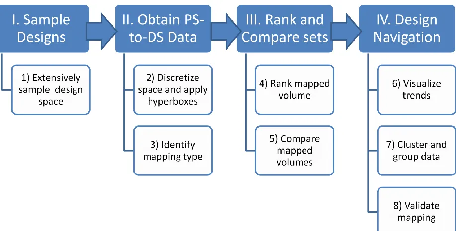
In this chapter, the research approach proposed in the thesis is outlined and discussed. The approach in Figure 3.1 is used to locate and analyze one-to-many mappings in multiobjective engineering problems. To facilitate the discussion of the approach, a sample problem – ZDT-3 (Zitzhler, 1999) – is simultaneously presented.
The proposed research approach to analyze design freedom contains a series of 8 steps. They are broken down into four major components, which are described below:
I. Sample Designs: Sample designs to obtain information on the performance values II. Obtain PS-to-DS data. Generate inverse data from the performance (PS) to
design space (DS). This step identifies mapping types and quantifies design freedom of selected locations in the performance space.
III. Rank and Compare sets. Rank the performances according to design freedom and compare design freedom across different locations in the performance space. IV. Design Navigation: Visualize design variables and identify mapping trends to
guide user decisions. This step supports designer decision making through validating mapping information and clustering designs.
3.1. Sampling the Design Space
The research approach requires that feasible performances are found. There are two sets of designs that are deemed of interest within the thesis. One is the set of Pareto-optimal designs. This set consists of highly-optimal designs, which designers identify to avoid inferior products. The other set of designs is chosen so that it covers the range of performances which are achievable in the multiobjective optimization problem, even if they are dominated designs.
This explanation begins with a review of the definition of a function. A function is a mapping between a variable that belongs to the domain of a function, to the range of the function (Lay. 2000). In the context of the current thesis, a function maps from design space to performance space. The function can be described either as a formula that describes the mapping, given in (3.1a), or through a mapping itself, given in (3.1b). It is assumed that a design can be presented as a vector of real numbers, , with performances given as multidimensional vectors of real numbers, .
Sampling designs of a given problem fills the mapping information in Equation (3.2). The first step of the research approach chooses how to sample the design space of a given multiobjective optimization problem. The choice occurs between the two objectives that are of particular interest, 1.) seeking optimal performances or 2.) seeking higher design freedom in dominated performances.
(3.2)
To identify a problem‘s Pareto frontier, MOGAs have been shown as an effective approach. They show robustness in generating optimal solutions in multiple settings, for both continuous and discrete problems. To optimize efficiency and evaluate a large number of designs, the thesis uses a software package from Sastry (Sastry, 2006) in identifying Pareto-optimal designs.
The research approach uses the two sets of designs that result from each method. The range of evaluated designs is 5000-10000 which is kept in the same order of magnitude between the two sets of designs. The design population is kept constant at the target level throughout the MOGA optimization. Thus, the population stays at q = 5000 or q = 10000 during the evolutionary stage. At the end of the optimization, any infeasible designs are discarded.
Under LHS, a list of designs configurations is generated which are first evaluated for feasibility. For example, for a target range of q = 5000 designs, a list of 1000 designs is generated and evaluated for infeasibility. The feasible designs are saved and a new list of 1000 sample design is generated and checked for feasibility. The process is continued until the target number of designs is reached or exceeded. Therefore, the LHS set can slightly overshoot the target number of designs.
The current sampling step completes the exploration of the multiobjective problem. The evaluation of sets of sampled designs allows us to consider performance-to-design information. In it, the binary pair ( is instead numerically presented as ( . The process is elaborated on in Section 3.2. The current step is illustrated on an example problem.
Application to a simple optimization problem
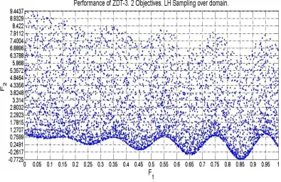
strategies and in (Zitzler, 2000) introduce a set of 6 test-bed optimization problems. This section presents initial analysis on a problem from the set, ZDT-3. The version presented in Equation (3.3) is an unconstrained multiobjective problem with two objectives and two design variables.
(3.3)
For
Figure 3.2. Feasible Performances of LH Sampling
The next sampling is an optimization procedure using the MOGA toolbox, supplied by (Sastry, 2006). There is a limit of 200 generations, after which the algorithm terminates. The design population is initiated through a random generation. The population size is set at 5000. The population undergoes 200 generations. In each generation, half of the designs are modified to explore for optimal values in new regions of the space. The supplied optimization toolbox, GAtbxm, requires a configuration file with the necessary input variables. The file is included in Appendix A.
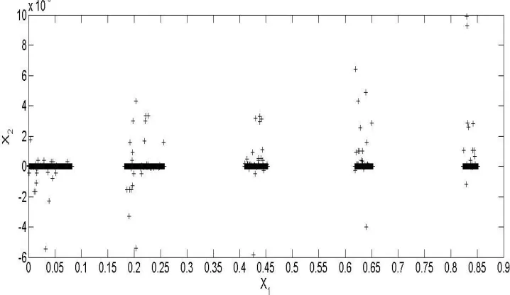
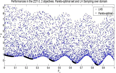
The Pareto-set is shown in Figure 3.4. The Pareto-optimal performances cover a range of [0, 0.8518] in F1 and a range of [-0.773, 1] in F2. The range of optimal performances in F2 is
significantly smaller for the Pareto-optimal set than for the LHS designs. The design space is shown in Figure 3.5. The generated set of optimal designs occupy a range of [0, 0.8518] in X1
Figure 3.4. Pareto-optimal performances for the two objectives
Figure 3.6. Pareto and LHS Performances of the studied function
3.2. Indifference thresholds discretization
The thesis uses indifference thresholds in quantifying design freedom. Designs are considered equivalent if they belong to a target hyperbox, which is characterized by a specified indifference threshold limit. The process is shown in (Ferguson, 2005ab). The step is used on both the performance and design variables.
Consumers can find themselves in a position to consider some similar performances to be equivalent. An example can be given for a customer comparing fuel economy of car models. A person with an indifference threshold of 1 MPG would not differentiate between cars that are listed to have 25 MPG or 26 MPG. A customer can find mileage information on the site fueleconomy.gov, which lists the mileage of a 2.4 L, 4 cylinder 2010 Chevrolet Malibu is rounded to 26 miles per gallon for a combined driving test cycle. The mileage for 2.5L 4 cylinder 2010 Ford Fusion FWD is listed as 25 MPG. For the example customer, these performances are within their desired target performance and therefore they are equivalent to each other.
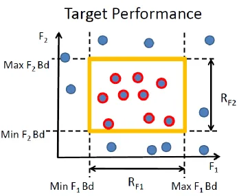
Consider the case for the performance in a two objective problem, shown in Figure 3.7. The designer chooses a two-dimensional indifference range vector , that has two components, RF1 and RF2. The indifference threshold is used to create boundaries of target performances.
target performance. The design space is discretized in a similar fashion using an indifference range vector .
Figure 3.7. Performance space box boundaries defining a target performance
an n-dimensional domain, ( . While investigating Research Question 2, the indifference threshold setting is varied between 0.1% to 10%.
To choose a performance indifference threshold, we assume a set of evaluated mappings M, as constructed in Equation (3.2), is already generated. The set can consist either of Pareto-optimal designs or feasible designs generated through LHS. For each set, the performance range is calculated as the multidimensional upper and lower bounds of performances ( . The indifference threshold is set at 5% of the range of each objective. It creates 20m hyperboxes in the m-dimensional space of considered performances in each set of mappings, M.
The indifference threshold values are therefore dependant on the particular set of mappings being studied. Nevertheless, the number of performance and design space boxes stays constant. The mappings cover different performance regions and therefore the indifference thresholds are scaled to correspond to the different regions.
The application of hyperboxes is given by distances from the centroid points in each particular box. There are 20m such points in performance space. The target centroid points in design space are 20n. Equation (3.5) describes how to construct each point, indexed under j and k respectively.
= (3.5a)
For a hyperbox, in performance space, any performance within the performance
indifference threshold maps to it, . Equation (3.6a) is a mapping function that groups the performances within the hyperbox bounds. Similarly, Equation (3.6b) maps indifference threshold discretizations in the design space.
(3.6a)
(3.6b)
The process groups equivalent performances together, while permitting the differentiation between dissimilar design configurations. Effectively, a mapping is created for each design between hyperboxes in the performance space and design space. Consequently, is presented as where and . The hyperboxes retain the same dimensionality of the original corresponding DS and PS, but exist in integer space. The mapping is then inverted to obtain the following performance-to-design space structure, as shown in Equation (3.7).
The discretization process quantifies design freedom in a 1-norm distance metric in both performance and design space. The designer assumes that customers measure performance within the performance indifference threshold. Furthermore, the designer assumes that differences in physical configurations are measured in each variable separately up to the design space indifference threshold.
Designers have the opportunity to uniquely define and modify hyperboxes in both the design space and performance space. The hyperbox mapping, as in Equation (3.7) can be extended to include some general functions and according to their individualized computational preferences. The function is generic to allow the designer to specify how to carry the step. The functions can be defined depending to the particular design application as in Equation (3.8).
(3.8a) (3.8b)
Application to a simple optimization problem