How to Make a Mudsparkler

(1)

University of South Carolina

Scholar Commons

Theses and Dissertations

2017

Confluence of Density Currents Produced by

Lock-Exchange

Hassan Ismail

University of South Carolina

Follow this and additional works at:https://scholarcommons.sc.edu/etd

Part of theCivil Engineering Commons

This Open Access Dissertation is brought to you by Scholar Commons. It has been accepted for inclusion in Theses and Dissertations by an authorized administrator of Scholar Commons. For more information, please [email protected].

Recommended Citation

Ismail, H.(2017).Confluence of Density Currents Produced by Lock-Exchange.(Doctoral dissertation). Retrieved from

(2)

Confluence of Density Currents Produced by Lock-Exchange

by

Hassan Ismail

Bachelor of Science

University of South Carolina 2011

Master of Science

University of South Carolina 2015

Submitted in Partial Fulfillment of the Requirements

for the Degree of Doctor of Philosophy in

Civil Engineering

College of Engineering and Computing

University of South Carolina

2017

Accepted by:

Jasim Imran, Major Professor

M. Hanif Chaudhry, Committee Member

Enrica Viparelli, Committee Member

Jamil Khan, Committee Member

(3)

c

Copyright by Hassan Ismail, 2017

(4)

Dedication

(5)

Acknowledgments

This work was possible thanks to funding support from the National Science

Foun-dation.

I would like to thank my dissertation committee for their time, constructive

feed-back, and guidance in completing this work. Foremost is Jasim Imran, my advisor,

mentor, major professor, and collaborator on research projects through my

gradu-ate studies. His encouragement and flexibility allowed me to investiggradu-ate a variety of

scholarly projects through my time at the University, and what I have learned under

his advisement goes far beyond the contents of the work presented here. Thank you

to the members of my committee, M. Hanif Chaudhry, Enrica Viparelli, and Jamil

Khan who have supported, questioned, and probed my work to ensure that I have

earned this doctorate, and the work itself can be given the name "dissertation" in the

truest meaning of the word.

I would also like to thank the water resources research group, Department of

Civil & Environmental Engineering, and the University of South Carolina. I can not

think of any fellow graduate student or post-doctoral researcher in the water resources

research group with whom I have not discussed, collaborated, or brain-stormed about

my research. Specifically, I would like to thank Lindsey LaRocque for her guidance

in the laboratory and in graduate school life. I have made a home at the University

of South Carolina over the course of my studies, and I want to thank the University

system which has treated me well for many years, and I hope I have and continue to

represent the University with integrity and pride.

(6)

in the Department of Civil & Environmental Engineering. Specifically I want to

ac-knowledge Anne Kawamoto, Patrick Blake, Russell Inglett, and Karen Ammarell.

Anne has always been helpful with organization of the research group. Patrick has

helped with information technology needs including helping me get started with

us-ing Linux operatus-ing systems which became critical to this work. Russell provided

laboratory support in all studies conducted in the laboratory. Finally, Karen has

helped with any procedural needs to ensure I followed all departmental and

univer-sity guidelines. I tell every student that I can, "If Karen is not your best friend yet

in this department, make sure she becomes that soon."

Most importantly, I want to acknowledge my family. My father, Mohamad, my

late mother, Randa, and my two brothers, Ahmad and Bassem: thank you all for

shaping me into the man I am today. And mom, I miss you and thank you for the

time we did have together. I want to thank my wife and best friend, Heather. Nothing

in this work would be possible without the support given by her; I could not ask for

more. Finally I would like to thank Heather for giving to me my joy, my son Gabriel.

(7)

Abstract

Density currents represent a broad classification of flows driven by the force of gravity

acting on a fluid with variable density. With examples of density currents including

turbidity currents, sand storms, salt wedges in tidal rivers, and oil spills, a great deal

of attention has been previously given to understanding the underlying mechanisms

of such flows and implications of those flows on fluid, species, and sediment transport.

Although documented confluences occur naturally in terrestrial and submarine

set-tings, little attention has been given to understanding the confluence of two density

currents.

This study furthers the state of knowledge on density current confluences by

systematically studying the unsteady flow phenomena and providing a methodology

for describing the flows based on the bulk properties in the pre- and post-confluence

density currents. Numerical simulations were conducted with experimental validation

in which the effect of the initial density difference, channel depth, and junction angle

were studied. The simulations revealed that the junction played a critical role in the

combined current’s bulk properties.

In the junction zone, the density currents accelerated and became thicker. After

the combined front continues downstream, an elevated plume of dense fluid remained

in the junction zone for some time. It was concluded for the range of densities tested,

that initial density difference has little effect on the bulk properties when

nondimen-sionalized. The role of the junction angle was isolated, and it is concluded that higher

junction angles result in higher peak velocity in the junction zone and a larger plume.

(8)

of the combined current have little dependence on junction angle further downstream.

The initial conditions (initial density, channel depth, and junction angle) are

com-bined via a Reynolds number giving an indication of the downstream oriented inertia

entering the junction zone from both upstream branches of the channel network.

Trends in bulk properties as functions of this Reynolds number are presented, but

at high values of Reynolds number, many bulk properties approach a constant value

(9)

List of Tables

Table 3.1 Experimental and numerical test cases and results of bulk properties. 17

Table 4.1 Case summary. D0/H0 = 1 indicates full-depth cases, andD0/H0

<1 indicates partial-depth cases. . . 31

Table 4.2 Constant upstream , peak, minimum, and constant downstream head thickness for each case. Thicknesses are normalized by channel depth and position is normalized by lock length mea-sured from the upstream wall. Empty entries indicate that no

constant value was reached. . . 32

Table 4.3 Plume thickness results for full-depth cases. The position is mea-sured from the upstream wall of the domain and is normalized

by the lock length. . . 33

Table 4.4 Results of the distance from the current nose to the location of maximum plume height, ∆X. The position is measured from the

upstream wall of the domain and is normalized by the lock length. 34

Table 4.5 Nose height results for full-depth cases. The position is measured from the upstream wall of the domain and is normalized by the

lock length. . . 35

Table 4.6 Froude number summary in each phase of flow. Location val-ues are normalized by lock length and are measured from the

upstream wall. . . 36

Table 4.7 Summary of near-bed maximum horizontal velocity. Locations are normalized by the lock length and measured from the

up-stream wall. Horizontal velocity is normalized byqg_o0Ho. . . 37

Table 5.1 Initial conditions for each junction angle. . . 59

(12)

Table 5.3 Froude number results for each case. The second peak and con-stant Froude number correspond to the post-confluence

reaccel-eration phase. . . 60

(13)

List of Figures

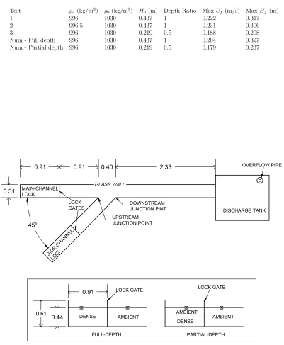
Figure 3.1 Plan and profile of the experimental flume for full- and

partial-depth cases. Units are in meters. . . 17

Figure 3.2 Comparison of front shape for the physical experiments and

simulations at 5s and 14s after the lock-gates were released. . . . 18

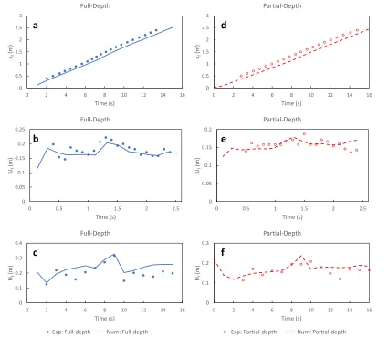
Figure 3.3 Comparison of bulk properties (front position, front velocity,

and front thickness) from the physical experiments and simulations. 18

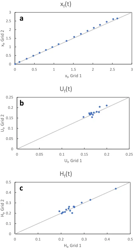
Figure 3.4 Comparison of simulation output from the grid 1 and grid 2 for

the full-depth case. . . 19

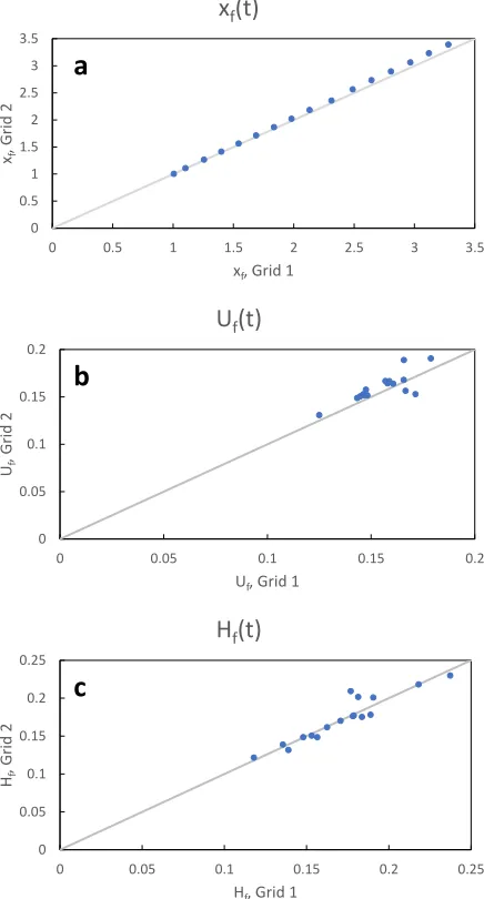
Figure 3.5 Comparison of simulation output from the grid 1 and grid 2 for

the partial-depth case. . . 20

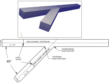
Figure 4.1 Computational grid and domain geometry. . . 38

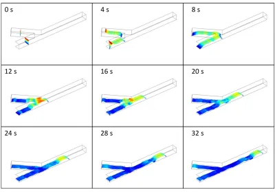
Figure 4.2 Typical propagation of the density currents for a full-depth case

(case 5). Colors indicate distance from the bed. . . 39

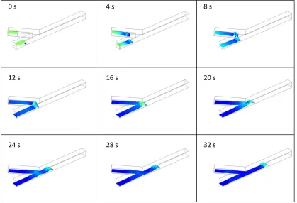
Figure 4.3 Typical propagation of the density currents for the

partial-depth case (case 11). Colors indicate distance from the bed. . . . 40

Figure 4.4 Propagation of the density current for case 9 along the main-channel centerline visualized as isolines of nondimensional

con-centration. . . 41

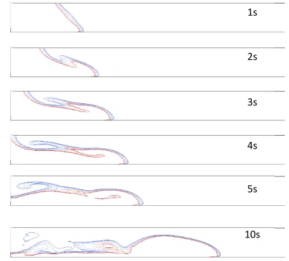
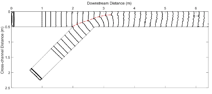
Figure 4.5 Time series of the near-bed front shape for case 5. Each output is separated by 0.77 nondimensional time units. The dash line

is the interpreted shear plane. . . 42

Figure 4.6 Time series of near-bed horizontal velocity and vertical velocity direction for case 5. Light shading indicates vertical velocity is

(14)

Figure 4.8 Head thickness versus front position for full-depth and

partial-depth cases. The symbology follows figure 4.7. . . 44

Figure 4.9 Plume thickness versus front position for full-depth and

partial-depth cases. The symbology follows figure 4.7. . . 45

Figure 4.10 Distance from the nose to the location of the plume, ∆X, versus

front position for full-depth and partial-depth cases. . . 46

Figure 4.11 Nose elevation versus front position along the main-channel cen-terline for the full-depth cases and partial-depth cases. The

symbology follows figure 4.10. . . 47

Figure 4.12 Froude number versus front position for the full-depth and

partial-depth cases. . . 48

Figure 4.13 Maximum near-bed horizontal velocity versus front position for full-depth and partial-depth cases. The symbology follows

fig-ure 4.12. . . 49

Figure 4.14 Pre-confluence trends in bulk properties with initial Reynolds

number. . . 50

Figure 4.15 Trends in ∆X with initial Reynolds number. . . 51

Figure 4.16 Post-confluence constant Froude number versus initial Reynolds

number. . . 51

Figure 4.17 Trends in nose height with initial Reynolds number. . . 52

Figure 5.1 Dimensions for the domain for each junction angle, θ. Linear

dimensions are in meters. . . 62

Figure 5.2 Typical propagation of the density currents for case 5 (H0 = 0.4 and ρ0 = 1025 kg/m3) for each junction angle. Colors indicate

distance from the bed. . . 65

Figure 5.3 Time series of the near-bed front shape for case 5 (H0 = 0.4 and ρ0 = 1025 kg/m3) for each junction angle. Each output is

separated by 0.77 nondimensional time units. . . 68

(15)

Figure 5.5 Nondimensional front velocity versus front position for each

junction angle. . . 74

Figure 5.6 Nondimensional front thickness versus front position for each junction angle. . . 77

Figure 5.7 Nondimensional trends in head thickness, Hf and plume thick-ness with ˆRe0. The front position is measured from the up-stream wall of the main-channel. . . 78

Figure 5.8 Nondimensional trends in maximum near-bed horizontal veloc-ity,Uh, with ˆRe0. . . 78

Figure 5.9 Nondimensional trends in ∆X with ˆRe0. . . 79

Figure 5.10 Nondimensional trends in nose height with ˆRe0. . . 79

(16)

Chapter 1 Introduction

1.1 Background

Density currents are flows driven by the force of gravity acting on a fluid with

vari-able density. They can occur in a number settings generated by both natural and

man-made phenomena including ocean currents driven by salinity and temperature

variation, turbidity currents, oil spills on sea surfaces, or salt wedges in tidal rivers

to name a few [Simpson, 1997].

Although density currents have been studied in laboratory and numerical models

[e.g., Keeulegan, 1949, Simpson and R. E. Britter, 1979, Parker et al., 1986, 1987,

Garcia and Parker, 1993, Kneller et al., 1999, Peakall et al., 2000, Kneller and Buckee,

2000, Peakall et al., 2007, Huang et al., 2008, Islam and Imran, 2008, Sequeiros

et al., 2010, Huang et al., 2012, Ezz et al., 2013, Janocko et al., 2013, Tokyay and

Garcia, 2013] and limited field observation [e.g., Prior et al., 1987, Normark, 1989,

Khripounoff et al., 2003, Paull et al., 2002, Xu et al., 2004, Vangriesheim et al., 2009,

Cooper et al., 2013], attention is almost exclusively given to behavior of these currents

in straight or sinuous channels. Although submarine channel confluences that convey

episodic density currents are evident in the geologic record [e.g., Canals et al., 2000,

Valle and Gamberi, 2011, Greene et al., 2002, Hesse, 1989, L’Heureux et al., 2009,

Mitchell, 2004, Paquet et al., 2010, Straub et al., 2011], and deltaic channel networks

passing salt wedges during tidal cycles have documented confluences as salt wedges

(17)

the author’s knowledge, the work of Ismail et al. [2016] represents the only controlled

investigation into the confluence of density currents.

Salt wedges, propagating due to tidal forcing, extend landward in coastal channels

beneath ambient riverine discharge. In such coastal channel systems, bifurcating

river channels act as confluences for salt wedge density currents during high tide

conditions when the flow is in the landward direction. Limited field studies have been

conducted with regard to tidal channels with salt wedge confluences [e.g., Buschman

et al., 2013, Warner et al., 2002, Sassi et al., 2011]. Buschman et al. [2013] observed

periodic variation in stratification in their field study of suspended sediment, salt,

and water fluxes in a tidal channel junction. They found that the bed level gradient

was relatively high in the junction compared with the straight-channel reaches due

to periodically high sediment transport capacity. Warner et al. [2002] concluded that

residual circulation in the junction zone of the Mare Island and Carquinez Straights

in San Francisco Bay were altered by phasing of landward-migrating currents. Sassi

et al. [2011] developed a numerical model of the Mahakam Delta channels in which

they studied the effects of the tidal discharge. They found that the salt wedges in

the system have a significant effect on the entire water column including the upper

zone of riverine discharge.

Submarine channel junctions which convey density currents have been identified

through field observation [e.g., Canals et al., 2000, Valle and Gamberi, 2011, Greene

et al., 2002, Hesse, 1989, L’Heureux et al., 2009, Mitchell, 2004, Paquet et al., 2010,

Straub et al., 2011]. Gamboa et al. [2012] interpreted and analysed 3D seismic data

to provide a detailed survey of submarine confluences and present a classification

scheme similar to that used for river confluences. Hesse [1989] and Klaucke et al.

[1998] identified extensive networks of converging drainage channels on the Labrador

(18)

applied fluvial hydrology principles to the submarine setting and recommended simple

relationships for erosion rates as a function of channel gradient and contributing area.

Straub et al. [2007] assessed submarine channel profiles and drainage areas on the

Monterey, CA and Brunei Darussalam continental slopes and found that submarine

scaling exponents were within the range of terrestrial observations despite differences

in physical processes.

Ismail et al. [2016] conducted a laboratory investigation on the confluence of

con-tinuous release density currents over an erodible bed. They found through their

phys-ical experiments, that models developed for confluences for subaerial rivers cannot

adequately predict separation zone dimensions, streamline deviation along the

junc-tion line, and maximum scour depth. They concluded that the upward convecjunc-tion of

dense fluid in the junction had a major impact on the flow dynamics and sediment

transport in the junction zone and downstream reach. The present work aims to

further the understanding of density current confluences through investigation of the

current front behavior in a confluence.

In work presented here, converging density currents at a channel confluence are

in-vestigated. Numerical experiments are conducted in a lock-exchange configuration to

study the transient phenomena. The flow conditions in the confluence are described,

and trends in the behavior at the junction based on initial and geometric conditions

are assessed and presented with proposed relationships.

1.1.1 Background on lock-exchange flows

Since many natural density currents are episodic in nature, researchers often perform

so called lock-exchange experiments to study their behavior. In a lock-exchange

scenario a vertical barrier, the lock gate, separates denser and lighter fluids which

are initially at rest. When the lock gate is removed, the denser fluid slumps below

(19)

produces a dense current propagating near the bed and a light current propagating

above the dense current. Shin et al. [2004] provides a review of previous lock-exchange

experimental work.

Two cases of lock-exchange experiments are conducted – full- and partial-depth

flow. In a full-depth condition, the dense fluid and light fluid have the same initial

depth, Ho, typically equal to the total channel depth. In a partial-depth condition,

the initial depth of the dense fluid, Do, is less than the entire channel depth, Ho (see

Shin et al. [2004], their figure 1).

Phases of Flow

Huppert and Simpson [1980] described the spreading of density currents produced by

lock exchange in three phases. The first phase is the slumping or constant velocity

phase. Following this is an inertial phase where the front speed is affected by

buoy-ancy and inertial forces. Finally, the current reaches the viscous phase during which

viscous effects overwhelm inertial forces, and viscosity and buoyancy are dominant.

In general, the front velocity,uf, begins as time-independent in the constant velocity

phase, followed by dependence as uf ∼t−1/3 in the inertial phase, then finally is an

additional time dependence in the viscous phase asuf ∼t−4/5.

In addition to these three phases, an initial acceleration phase is described by some

researchers [Martin and Moyce, 1952a,b, ¨Hartel et al., 1999, Cantero et al., 2007]. The

acceleration phase is short lived and describes the flow between the initial, at-rest

state of the dense fluid and the constant velocity phase. In the acceleration phase,

the front velocity sharply increases to a peak value followed by a slight decrease to

the constant value. Cantero et al. [2007] attribute the reduction at the end of the

acceleration phase to interface friction causing roll-up of the current in the early

(20)

velocity, it is convenient to define a Froude number as

F = quf g0hf

(1.1)

where uf is the front velocity, g

0

=g(ρ−ρa)/ρ is the reduced gravity, hf is the

front thickness, ρ is the current’s density andρa is the ambient fluid density.

Benjamin [1968] proposed an analytical solution for a two-dimensional cavity using

a reference frame moving with the front. In his constant velocity analysis, Benjamin

[1968] did not distinguish the current head versus the body and theorized that the

Froude number is only a function of the fractional current depth,hf/Ho, wherehf is

the current depth andHo is the depth of the channel. Benjamin [1968] found that for

energy-conserving currents,F = 0.5. For the case of maximum dissipation, Benjamin

[1968] found that F = 0.527. In the limit of infinite ambient water depth, hf → 0,

the analytical theory of Benjamin [1968] results in F = 1.41.

Huppert and Simpson [1980] proposed an empirical expression for Froude number

as a function of the fractional current depth based on the body of the current. They

found that F = 0.445 for the energy conserving case of hf/Ho = 0.5. For the limit

of infinite ambient depth, their empirical expression yieldsF = 1.19.

Shin et al. [2004] expanded the analysis of Benjamin [1968] by including the effects

of the reverse ambient bore interaction with the dense current. Their model was based

on the initial depth of dense fluid, Do, and they found that for full-depth cases (Do

=Ho), the theory was identical to that of Benjamin [1968].

The inertial phase of flow begins when the light current propagating in the

up-stream direction reflects off the upup-stream boundary, and the resulting wave reaches

the front [Rottman and Simpson, 1983]. The behavior of the density current in this

stage has been studied by several researchers [Fay, 1969, Fannelop and Waldman,

1971, Hoult, 1972, Huppert and Simpson, 1980, Rottman and Simpson, 1983]

(21)

¯

xf =ζ(¯hox¯o¯t2)1/3 (1.2)

¯ uf =

2

3ζ(¯hox¯o)

1/3_¯_t−1/3 _(1.3)

where the overbar represents a nondimensional value (Ho is the length scale,

Uo = (g

0

Ho)1/2 is the velocity scale, and Ho/Uo is the time scale), ¯xf and ¯uf are

the dimensionless streamwise front position and front velocity, respectively, ¯hox¯o

rep-resents the initial dense fluid volume per unit width, andζ is a shape factor and was

prescribed by Hoult [1972] as 1.47 and by Huppert and Simpson [1980] as 1.6.

As the current continues to propagate, the inertial phase causes the current to

decelerate with time. Thus the ratio of inertial to viscous forces decreases, i.e., the

Reynolds number, Re = ufh/ν, decreases. Here, ν is the kinematic viscosity. Once

the Reynolds number is sufficiently small, and the viscous forces become comparable

to the buoyancy forces, the current enters the viscous phase. Similar to the solutions

for the inertial phase, the viscous phase front position and velocity can be described

by the initial volume of the release but with an additional dependence on Reynolds

number and time. The equations will not be repeated here but can be found in Hoult

[1972] and Huppert [1982].

Current Thickness

To avoid ambiguity in defining the current depth, a similar equivalent depth method

is adopted here as was presented by Shin et al. [2004], Marino et al. [2005], Cantero

et al. [2007]. First, a nondimensional density is defined as

¯

ρ= ρ−ρa ρo−ρa

(1.4)

(22)

equivalent depth can be computed by integration of the vertical density profile. In

the present work, ¯ρ = 0.5 is used as the threshold for the dense-ambient interface to

define the current depth as h=h(x, z, t)|ρ¯=0.5.

1.2 Outline

In work presented here, converging density currents at a channel confluence are

in-vestigated. Numerical experiments are conducted in a lock-exchange configuration to

study the unsteady phenomena. The flow conditions in the confluence are described,

and trends in the behavior at the junction based on initial and geometric conditions

are assessed and presented with proposed relationships.

Chapter 2 introduces the governing equations and model. Solution algorithms

utilized in this work are discussed. Chapter 3 presents the physical experiments

conducted for model validation. Three tests were run of full- and partial-depth density

current confluence in a 45◦ junction in the Hydraulics Laboratory at the University of

South Carolina. Assessment of the front velocity and front thickness were made and

compared to numerical model results. Additionally, refined grid numerical simulations

were run to verify grid independence of trends in bulk properties of the flow.

Chapter 4 provides insight into the unsteady phenomena of density current head

confluences. Nine full-depth cases and three-partial depth cases are presented in

which initial lock depth and density difference were varied for a 45◦ junction angle. A

discussion of the observed phenomena and results are presented on the front velocity,

current depth, nose height, and near-bed horizontal velocity before and after the

confluence. Finally, the results are correlated to the initial conditions leading to

predictive relationships for the effect of the junction.

Chapter 5 continues the investigation into density current head confluences by

systematically investigating the effect of the junction angle. Five junction angles are

(23)

of 45 cases). First, the effect of the junction angle on the bulk properties is isolated.

Then, the initial conditions, including the junction angle, are combined into a single

parameter representing the downstream inertia entering the junction zone for the

(24)

Chapter 2 Numerical Model Description

The three-dimensional, unsteady simulations were implemented in the open-source

computational fluid dynamics toolbox, OpenFOAM [OpenFOAM, 2011a,b].

Open-FOAM is a compilation of modifiable C++ libraries which are used to create

exe-cutable solvers and utilities. Solvers are compiled and run to solve specific continuum

mechanics problems, and utilities are executables used for pre- and post-processing

data for use with a solver (e.g., mesh generation, initial condition set-up, solution data

visualization, etc.). The modifiable executables allow for the creation of customized

solvers and utilities for specific problems not handled by pre-compiled solvers within

the toolbox.

The twoLiquidMixingFoamsolver in OpenFOAM, which solves the flow equations

for two miscible, incompressible fluids was used to solve the governing equations.

Simulations were set up to consider water and salt water as the two fluids. Since the

solver considers two completely miscible fluids, the resulting simulation models the

behavior of density currents produced by a solute or temperature difference. A large

eddy simulation (LES) approach was employed with a Smagorinsky-Lilly

subgrid-scale (SGS) closure [Smagorinsky, 1963, Lilly, 1966], and dynamic time stepping was

used to improve stability based on the Courant-Friedrichs-Lewy condition [Courant

et al., 1928].

2.1 Governing Equations

(25)

∂ρ ∂t +

∂(ρui) ∂xi

= 0 (2.1)

∂(ρui)

∂t +

∂(ρujuj) ∂xj

= ∂

∂xj "

µ ∂ui ∂xj

+∂uj ∂xi ! −2 3µ ∂uj ∂xi δij # − ∂p ∂xj

−∂(ρτij) ∂xj

+ρgj (2.2)

where ρ is the bulk density, t is time, uj is velocity in the j direction, xj is a

Cartesian direction, µ is the dynamic viscosity, δij is the Kronecker delta, p is the

pressure,τij is the Reynolds stress, and gj is the gravity vector.

The Reynolds stress term in LES modeling is handled using spatial filtering and

is taken to be

τij =−2νtS¯ij (2.3)

where νt is the turbulent eddy viscosity, and ¯Sij is the rate of strain tensor.

By including equation 2.3 into the momentum equation (equation 2.2), the LES

momentum equation takes the form

ρ∂ui ∂t +ρui

∂uj ∂xj

=− ∂p

∂xj

+σ ∂ρ ∂xj

+ρ∂σ ∂xj

+ρgj (2.4)

σ = (ν−νt) ∂ui ∂xj

+∂uj ∂xi ! −2 3ν ∂ui ∂xj

δij (2.5)

To close the momentum equation, the Smagorinsky-Lilly SGS model is used where

νt= (C∆)2|S| (2.6)

where C is a constant and ∆ is the filter length computed as the cube root of the

cell volume.

(26)

ρ=Xckρk (2.7)

where ck and ρk are the concentration and density of species k, respectively. For

one fluid and a species within that fluid, i.e., water and dissolved salt, equation 2.7

becomes

ρ =csρs+ (1−cs)ρw (2.8)

where cs and ρs are the concentration and density of the salt water, respectively,

and ρw is the density of the ambient water.

The concentration,cs, of the species is conserved and solved for using the species

continuity equation as

∂cs

∂t +

∂ ∂xj

(uj−vsδijcs) = ∂ ∂xj

νt Sct

∂cs ∂xj

!

(2.9)

where vs is the fall velocity and equal to zero for a dissolved species or heat and

Sct is the turbulent Schmidt number.

2.2 Solution Algorithm

For efficient solution of the governing equations, the PIMPLE (PISO-SIMPLE)

al-gorithm is utilized [OpenFOAM, 2011a,b]. The PIMPLE alal-gorithm is a merger of

the Pressure Implicit with Splitting of Operators (PISO) algorithm [Issa, 1986] and

Semi-Implicit Method for Pressure-Linked Equations (SIMPLE) algorithm [Ferziger

and Perić, 2001].

The PISO algorithm splits operators into an implicit predictor step and

mul-tiple explicit corrector steps. In OpenFOAM, velocity is first predicted using the

known pressure from the previous time step, then the pressure is corrected using

(27)

pres-sure. SIMPLE uses relaxation factors to iteratively adjust the corrected variables for

smooth convergence. The PIMPLE algorithm takes advantage of the PISO method

with the addition of relaxation factors for smooth convergence from the SIMPLE

method. This allows for stable solution of the coupled pressure-velocity equations to

a prescribed threshold at Courant numbers greater than one.

The generalized geometric-algebraic multi-grid (GAMG) and Gauss-Seidel smooth

solvers were utilized to solve discretized equations. The advantage of GAMG is

that it first generates a solution for a geometrically coarsened grid which is then

used as an initial solution for the specified finer grid resulting in a faster solution

of matrices. Discretized terms in partial differential equations are solved using the

standard second-order accurate Gaussian finite volume integration method. The first

order accurate Euler time discretisation scheme and second order accurate Gauss

linear divergence scheme were utilized. Cell face values are interpolated between cell

(28)

Chapter 3 Physical Experiments & Model Validation

Before applying the numerical model introduced in Chapter 2 to the test cases,

phys-ical experiments were conducted for model validation. Three experiments were

con-ducted in a horizontal, 45◦_{: two involving full-depth lock-exchange cases and one}

partial-depth case. The results from the physical experiments, including front

posi-tion, front velocity, front thickness, and front shape are compared with the results

from the numerical model.

3.1 Model Set-up

The physical model geometry can be seen in figure 3.1. The bed of the horizontal

flume was made of wood, and the walls were made of wood except for the longest

wall along the main- and downstream-channels which was acrylic glass for flow

vi-sualization. The flume consisted of two upstream reaches each with 1.83 m length,

0.305 m width, and 0.61 m depth. The upstream channels meet at the upstream

junction point and continue to the downstream reach. The downstream reach then

discharges into a large tank with an overflow pipe to ensure constant ambient water

depth during testing. Each upstream reach was equipped with a thin gate at the

midpoint of the upstream reaches (0.915 m from the extreme upstream walls) and

lifting mechanism. The main-channel centerline and wall of the flume were marked

with a scale to track the current’s progression and size.

Each test involved closing and sealing the two gates and filling the flume

(29)

0.437 m. For the full-depth tests, each lock was filled with a premixed saltwater

solution with a density of 1030 kg/m3 _{to the same depth as the ambient water. For}

the partial-depth test, the lock was filled with saltwater for half the depth with

am-bient water above. Mixing of the lock fluid in the partial-depth case was avoided by

first filling the ambient water to the prescribed depth followed by slowly injecting

the dene fluid near the bed of the flume within the locks. Samples of the dense fluid

were obtained for the partial-depth case before release to verify the density had not

changed.

Each test was initiated by simultaneously lifting the two lock gates. To ensure

the gates lifted simultaneously, they were tethered together using steel cable, and a

single counter-weight was released to lift the gates. The density currents then formed

in a relatively short time after the release before reaching the junction zone. Then,

they combined in the junction zone and were allowed to continue downstream. The

currents were tracked visually by dying the saltwater before testing and tracking

movement with two high-definition video cameras positioned along the main channel

perpendicular to the main- and downstream-channels’ acrylic glass wall. The

cap-tured video for each case was split into individual frames (at a rate of 60 frames/s),

and the current position as a function of time along with the height of the current

were digitized for analysis.

3.2 Results

A summary of the test cases and results of bulk properties of the physical experiments

can be seen in table 3.1. The full-depth case was repeated to ensure repeatability

of the tests, and it can be seen from the results that there was only 3.7% difference

between the two test runs in terms of maximum front velocity and 3.4% difference in

(30)

3.3 Numerical Model Performance

The numerical model was applied to the test cases seen in table 3.1. Figure 3.2 shows

a qualitative comparison between the front shape from the physical experiment and

numerical model at 5s and 14s from the initiation of the current. At 5s, the current

had not yet reached the junction zone, and at 14s the front is in the downstream reach.

The general trend in the front shape between the experimental and numerical results

does not greatly vary in these two snapshots. Figure 3.3 presents the time series of

front position, front velocity, and head thickness along the main-channel centerline for

the physical experiments and numerical model. Although some variability in the data

is noted, the bulk properties and trends in the data agree well. Agreement between

the physical experiments and numerical model in terms of the bulk properties are

good with differences in maximum front velocity and maximum head thickness of

8.1% and 3.3% for the full-depth cases and 4.8% and 13.9% for the partial-depth

cases.

The numerical model was applied to the physical experiments using a proposed

grid resolution (grid 1) that is later to be applied to the numerical test cases presented

in the remainder of this work. To ensure the grid resolution was sufficient to capture

the bulk property characteristics of the flow phenomena, the validation tests were

reassessed with a refined grid (grid 2). Grid 2 consists of quadruple the number of

grid points as grid 1 by refinement of the horizontal resolution by a factor of two in

each direction. From figure 3.2 it can be seen that grid 2, the refined grid, captures

greater detail in the interface between the dense and ambient fluid, but bulk properties

do not differ. Figures 3.4 and 3.5 present a comparison of the simulations with very

close agreement between the two grids. This indicates that the grid 1 sufficiently

captures the flow phenomena is terms of bulk properties which is of interest in this

(31)

3.4 Summary

This chapter presented the methodology, results, and analysis of physical experiments

intended to validate the proposed numerical model and solution grid. Experiments

were conducted in a horizontal, asymmetric junction flume with gates equipped in

each upstream reach. Three physical experiments were conducted: two were

full-depth lock-exchange tests which were repeated to verify the consistency of the

exper-imental results, and the third was a partial-depth case.

Video cameras were used to capture the front position, front velocity, and head

thickness as a function of time. Dye was used for flow visualization and to

iden-tify the interface between the density current and ambient fluid. The repeatability

test showed good agreement indicating the experimental apparatus returns consistent

results across all tests.

The numerical model was applied to identical cases as the physical experiments

with a grid resolution equal to that presented in the later chapters of this work. The

shape of the current captured during the physical experiments matched well with

the numerical model results, and bulk properties were captured with the highest

difference being the maximum head thickness for the partial-depth case with 13.9%

difference. The rest of the bulk properties investigated were well below 10% difference

in the experimental and numerical results.

The numerical simulations were repeated for both the full- and partial-depth cases

with a refined grid (grid 2). The results indicate that the simulation output had little

variation between grid 1 and grid 2, thus the coarser grid, grid 1, is used for the

(32)

Table 3.1: Experimental and numerical test cases and results of bulk properties.

Test ρa(kg/m3) ρ0(kg/m3) H0(m) Depth Ratio MaxUf (m/s) MaxHf (m)

1 996 1030 0.437 1 0.222 0.317

2 996.5 1030 0.437 1 0.231 0.306

3 996 1030 0.219 0.5 0.188 0.208

Num - Full depth 996 1030 0.437 1 0.204 0.327

Num - Partial depth 996 1030 0.219 0.5 0.179 0.237

MAIN-CHANNEL LOCK

SIDE-CHANNEL LOCK

UPSTREAM JUNCTION POINT

DOWNSTREAM

JUNCTION PINT _{DISCHARGE TANK}

LOCK GATES

OVERFLOW PIPE

0.91 0.91 0.40 2.33

45° 0.31

GLASS WALL

LOCK GATE

DENSE

DENSE AMBIENT

AMBIENT

AMBIENT LOCK GATE

FULL-DEPTH PARTIAL-DEPTH

0.44

0.61

0.91

(33)

0 0.1 0.2 0.3 0.4 0.5

0 0.2 0.4 0.6 0.8 1 1.2 1.4 1.6 1.8 2

Di stance from B ed ( m)

Downstream Distance (m) 5 s

EXP Grid 1 Grid 2

0 0.1 0.2 0.3 0.4 0.5

1.4 1.6 1.8 2 2.2 2.4 2.6 2.8 3 3.2 3.4 3.6

Di stance from B ed ( m)

Downstream Distance (m) 14 s

Figure 3.2: Comparison of front shape for the physical experiments and simulations at 5s and 14s after the lock-gates were released.

0 0.5 1 1.5 2 2.5 3

0 2 4 6 8 10 12 14 16

xf (m) Time (s) Full-Depth 0 0.5 1 1.5 2 2.5 3

0 2 4 6 8 10 12 14 16

xf (m) Time (s) Partial-Depth 0 0.05 0.1 0.15 0.2 0.25

0 0.5 1 1.5 2 2.5

Uf (m) Time (s) Full-Depth 0 0.05 0.1 0.15 0.2

0 0.5 1 1.5 2 2.5

Uf (m) Time (s) Partial-Depth 0 0.1 0.2 0.3 0.4

0 2 4 6 8 10 12 14 16

Hf

(m)

Time (s)

Full-Depth

Exp: Full-depth Num: Full-depth

0 0.1 0.2 0.3

0 2 4 6 8 10 12 14 16

Hf

(m)

Time (s) Partial-Depth

Exp: Partial-depth Num: Partial-depth

b a c e d f

(34)

0 0.5 1 1.5 2 2.5 3

xf

, Gr

id 2

xf, Grid 1

x_f(t)

0 0.05 0.1 0.15 0.2 0.25

Uf

, Grid 2

Uf, Grid 1

U_f(t)

0 0.1 0.2 0.3 0.4 0.5

Hf

, Gr

id 2

Hf, Grid 1

H_f(t)

b

a

c

(35)

0 0.5 1 1.5 2 2.5 3 3.5

xf

, Gr

id 2

xf, Grid 1

x_f(t)

0 0.05 0.1 0.15 0.2

Uf

, Grid 2

Uf, Grid 1

U_f(t)

0 0.05 0.1 0.15 0.2 0.25

Hf

, Gr

id 2

Hf, Grid 1

H_f(t)

b

a

c

(36)

Chapter 4 Confluence of Density Currents in a 45

◦

Junction

This chapter presents numerical tests and results of the confluence of density currents

in a horizontal channel with 45◦junction angle. Nine cases of full-depth lock-exchange

and three cases of partial-depth lock-exchange confluences were tested and assessed.

First, the test conditions are presented followed by a discussion of the general trends

in the flow phenomena, then the bulk properties of the flow are analyzed as a function

of the initial conditions. Finally, the initial conditions are combined into an initial

Reynolds number and predictive equations are presented.

4.1 Initial & Boundary Conditions

The computational domain consisted of an asymmetrical junction of two horizontal

channels and a downstream channel (figure 4.1). The lock length, Lo, was 1 m, the

distance from the upstream edge of each channel to the upstream junction point was

2 m, the channel width, b, was 0.5 m, and the junction angle was 45◦. At the start

of each simulation, each lock was filled with dense water, and the rest of the domain

with ambient water.

For each case, the only changes in the domain were the height of the channel

(0.2, 0.4, and 0.5 m) and the number of vertical grids so that the vertical resolution

remained consistent across all cases (the same grid resolution established in Chapter

(37)

cases of 0.2 m, 0.4 m, and 0.5 m channel height. The grid size was 0.005 m, 0.03 m,

and 0.015 m in the vertical, down-channel, and cross-channel directions, respectively

(relative to the main-channel).

All boundaries were considered walls. Thus no mass flux through any boundary

was allowed. The bottom and side walls were rough boundaries and treated with a

no-slip condition for velocity. The initial condition for each case included a stationary

volume of dense water in each upstream channel’s lock. The release of the dense fluid

was instantaneous, and output was collected for analysis every one second of flow

time. The initial time step was set to 0.1 seconds which was dynamically adjusted

during the simulations to limit the Courant number, Co ≤ 1 for improved numerical

stability.

4.2 Numerical Experiments

The numerical model was applied to 12 density current cases. The first nine cases are

full-depth releases in which initial density difference and channel depth were varied.

The next three cases are partial-depth cases in which only initial density difference

was varied. Table 4.1 lists a summary of the conditions for each case. The channel

depth, H0, is used as the length scale, U0 = (g 0

H0)1/2 is used as the velocity scale,

and t0 = H0/U0 is used as the time scale throughout this work. The initial density

difference and channel depth are combined to assess the combined impact of these

variables through the initial Reynolds number,Re0, defined as Re0 = q

(g₀0H3 0)/ν2

(38)

4.3 Results & Analysis

4.3.1 Typical Behavior

This section presents the typical behavior of the junction cases. The general trends in

the full- and partial-depth cases are assessed in terms of propagation and confluence,

and nose shape.

Current Propagation

Figure 4.2 illustrates the typical propagation of the density currents as they are

released, combine in the junction zone, and continue downstream visualized by the

dense-ambient interface (¯ρ = 0.5). The color contours indicate elevation from the

bed. The density currents form in a short distance in the upstream reaches where

the dense-ambient interface is relatively smooth. As the currents combine in the

junction zone, the interface rises behind the front. After the head has cleared the

junction zone, the interface remains high in the junction zone near the downstream

junction point, and the interface is no longer smooth except just behind the combined

current’s nose. The elevated plume in the junction falls thereafter as the bulk of the

fluid continues downstream with a distinct and detached head.

Figure 4.3 shows a typical partial-depth case. As compared with the full-depth

case, the partial-depth case behaves similarly but propagates more slowly in the

downstream reach and with a more distinct head throughout.

The typical behavior of the current along the main-channel centerline can be

seen in figure 4.4. The plot shows isolines of constant nondimensional density. Note

that at 10s, the front has already passed the junction zone and interaction with the

(39)

Near-bed Front Shape % Velocity

Figure 4.5 shows the near-bed location of the density current in time. In this plot, each

output interval is 0.77 nondimensional time units. The near-bed plane is defined as

the upper edge of the first cells in the bed-normal direction. In each upstream reach,

the front shape is relatively smooth. In the junction zone, the side-channel current

extends into the junction first near the upstream junction point and begins to rotate

as the main-channel current enters the junction. Note the retreat of the side-channel

current as the fronts reach the downstream junction point. Further downstream, the

front has a more distinct lobe-and-cleft shape as is typical of density currents. The

absence of the lobe-and-cleft shape in the upstream reaches is due to the length of

the upstream channels. The lobe-and-cleft pattern becomes more pronounced as a

density current travels longer distances as reported by Cantero et al. [2007]. There

is a clear shear plane highlighted in the figure. This shows the separation of the

contributing currents from each upstream reach as they pass through the junction

zone. Further downstream, the currents mix and form a combined current. There was

no appreciable difference in the trends observed in the full-depth versus partial-depth

cases.

Figure 4.6 shows the near bed horizontal velocity vectors with shading indicating

the direction of the vertical velocity component; the light shade means the vertical

velocity is away from the bed. Superimposed in this figure is the near-bed front

position. It is clear that as the currents combine in the junction zone there is a

distinctive three-dimensional pattern in velocity with fluid along the shear plane

moving towards the bed. Further downstream the pattern of vertical velocity becomes

less obvious. In the downstream reach, where the lobe-and-cleft pattern in the front

shape is observed, vertical velocity can be seen to move towards the bed in the lobes

(40)

earlier work of Cantero et al. [2007].

Bulk Property Behavior

The bulk properties of all test cases are presented in figures 4.7 - 4.13. In these plot,

the junction zone extends fromxf/L0 = 2 to xf/L0 = 2.71.

As observed in figure 4.7, the position versus time collapses over initial density

difference and only differs for different values of H0. The same collapse is observed

for the partial-depth cases.

As the currents reach the junction zone, the current thicknesses increases (figures

4.8 and 4.9) and continues to increase until the head exits the junction zone. From

the plot of ∆X (figure 4.10), the location of the maximum thickness is near the head

when it enters the junction (∆X approaches 0 near xf/L0 = 2). This is followed by

increasing ∆X for the full-depth cases indicating that the elevated plume observed in

figure 4.2 remains in the vicinity of the junction as the head continues downstream

for some time. For the partial-depth cases, ∆X remains small indicating the head

of the current is always the thickest part of the current and no elevated plume is

observed (see figure 4.3).

For most full- and partial-depth cases the nose height, defined as the vertical

dis-tance from the bed to the downstream-most location of the current front, experiences

a slight peak in the junction zone. This observation follows that of Ismail et al.

[2016] that the main-channel current lifts above the side-channel current in the initial

mixing in the junction zone.

The front velocity behavior, normalized as a Froude number,F, shows distinctive

behavior atypical of straight-channel lock-exchange flows. Figure 4.12 showsF versus

nondimensional front position along the main-channel centerline for the full- and

partial-depth cases. Initially, the currents experience an acceleration phase to a first

(41)

expected since the currents have not yet reached the junction zone so they behave

as typical lock-exchange flows. In the junction zone however, the currents in all

cases experience a distinctive reacceleration to a second, global peak velocity. This

peak velocity always occurs near the downstream junction point (nearxf/L0 = 2.71)

and is followed by a post-confluence constant velocity phase. This reacceleration is

attributed to energy input from the side-channel current in the junction zone. Far

downstream, the currents enter the inertial phase where deceleration occurs gradually

as a function of time.

The maximum near-bed horizontal velocity is assessed and nondimensionalized

similarly to the front velocity (nondimensionalized by qg0_oHo). The maximum

near-bed horizontal velocity plot (figure 4.13) show similar trends in the early stages of

the release in which the currents undergo a sharp acceleration of horizontal velocity

followed by a constant value until reaching the junction zone. In the junction, a

small peak in the near-bed horizontal velocity occurs near the upstream junction

point (xf/L0 = 2). A third peak is then observed near the downstream junction

point (xf/L0 = 2.71). The second peak is attributed to increased flux of dense

fluid into the junction zone causing the currents to accelerate, and the third peak is

associated with the confinement of the combined mass of dense fluid to the width of

the downstream channel. In general, unlike the trends in Froude number, the global

maximum near-bed horizontal velocity occurs after the initial acceleration phase, but

the junction causes the currents to locally accelerate in all cases. Far downstream

in the inertial phase of the front velocity, all full-depth cases show convergence of

near-bed horizontal velocity to a value of approximately 0.27 regardless of initial

conditions. The partial-depth cases also appear to converge to a value of 0.2 far

(42)

4.3.2 Effect of Initial Conditions

The bulk properties are compared quantitatively in terms of front position, head

thickness, plume thickness in the junction, nose elevation, front velocity, and

max-imum near-bed horizontal velocity along the main-channel centerline. In addition,

the distance from the nose to the location of the maximum plume thickness, ∆X,

is assessed. Nondimensionalized results appear in figures 4.7 - 4.13. Extracted bulk

properties from these figures are presented in tables 4.2 - 4.7. These bulk properties

include constant and peak values of head thickness, plume thickness, ∆X, nose

eleva-tion, Froude number, and maximum near-bed horizontal velocity. Additionally, the

front position at which these parameters occur is listed in the tables.

In general, almost no trends appear in the bulk properties as a function of the

initial density, ρ0. Most plots (see figures 4.7 - 4.13) show collapse over ρ0. The peak

Froude number (see table 4.6) does decrease with increasing initial density for the

cases of H0 = 0.5 m, but this trend weakens for H0 = 0.4 m and is nonexistent for

H0 = 0.2 m. This trend also occurs for the partial-depth cases.

Trends appear in the bulk properties as a function of the initial channel depth,

H0. It can be seen in the tabulated results that the pre-confluence Froude number is

a function of H0. As expected, before the junction effects the flow properties, higher

H0 shifts the first peak Froude number downstream, and the constant velocity phase

Froude number is higher.

After the confluence, the front thickness, plume thickness, and ∆X are functions

of H0. Both the front thickness and plume thickness peak values do not change

significantly with H0, but the peaks occur further downstream with increasing H0.

Additionally, at lower H0, the minimum head thickness after the peak is lower with

smaller H0. With higher initial H0, the ∆X results suggest that the thickest part of

the current, the plume thickness, remains further behind the nose. This is intuitive

(43)

4.3.3 Effect of Initial Reynolds Number

Data extracted from the results are used to assess trends based on the combined

effects of the initial density difference and channel depth using the initial Reynolds

number defined as Re0 = q

(g₀0H3

0)/ν2, where ρ0 is the initial density of the dense

fluid in the lock, ρa is the ambient fluid density, and ν is the kinematic viscosity of

water. Tables 4.2 - 4.7 list the extracted data.

Before the confluence, trends in Re0 appear to be similar to those observed in

terms ofH0. At high Re0, the initial peak Froude number occurs further downstream

for both full- and partial-depth cases, and the constant velocity phase Froude number

also increases with higher Re0. Additionally, the first peak head thickness linearly

decreases with increasing Re0 for the full-depth cases (figure 4.14). In the

partial-depth cases, the first peak Froude number was independent of Re0.

During and after the confluence, many results show some dependence on Re0 but

only at certain values for the full-depth cases. Specifically, the minimum ∆X in the

junction zone after the first peak shows two modes, one for low Re0 which is constant

around 0.2, and another for high values of Re0 around 0.48 (figure 4.15). The second

peak value of ∆X has similar bimodal behavior for low and high Re0. However, at

higher Re0, the location of minimum ∆X and second peak ∆X both shift downstream

slightly with higher Re0. The post-confluence constant Froude number appears to

increase with increasing Re0 at lower Reynolds numbers (figure 4.16). This trend

diminishes at higher values of Re0 where an approximately constant value of F =

0.56 is observed.

The behavior of the nose height along the main-channel centerline for the

full-depth cases has the most dependence on Re0. With increasing Re0, the maximum

nose height, second constant nose height, and second peak nose height all linearly

(44)

cases, the partial-depth cases showed no appreciable dependence on Re0 during and

after the confluence.

4.4 Summary

Results and analysis of simulations of density current confluences in a 45◦ junction

in a lock-exchange arrangement have been presented. The focus of this study is to

describe the behavior of the head of the currents as they form upstream, combine

in the junction zone, and progress downstream as a single current. In addition to

describing the behavior, implications of changing initial conditions (excess density

and channel depth) are included in the analysis. Trends in initial Reynolds number

dependence were identified and presented.

After the release of the density currents, they formed in a relatively short

down-stream distance before reaching the junction zone. The currents combined in the

junction zone while they were in the constant velocity phase. They reaccelerated to

a global peak value near the downstream junction point with a distinctive rise in

thickness in the junction. As the combined current continued downstream, the

full-depth cases left an elevated plume of dense fluid in the junction which later subsided.

The partial-depth cases showed different behavior in the sense that the thickest part

of the current remained near the head at all times, and no elevated plume was

ob-served. The reacceleration and post-confluence constant velocity phases are unique

to the confluence phenomena versus straight-channel lock-exchange flows indicating

the combined current re-initiates after the initial mixing in the junction. A faster and

larger current is formed by the combining currents which propagates downstream.

When nondimensionalized, all bulk properties of the pre- and post-confluence

current collapsed over initial density,ρ0. Some dependence on the initial lock-depth,

H0 was observed. As expected, the front velocity, nondimensionalized as a Froude

(45)

the confluence, the front thickness, plume thickness and ∆X showed dependence on

H0.

The two initial conditions for each case were combined as an initial Reynolds

number, Re0, to assess trends. Before the confluence, higher values of Re0 caused a

downstream shift of the peak Froude number for all cases. Also, the pre-confluence

peak head thickness linearly decreases with increasing Re0 for the full-depth cases.

After the confluence, most bulk properties showed some dependence on Re0 but with

diminishing dependence at high values of Re0. The post-confluence constant Froude

number increases with Re0 at lower Reynolds numbers, but the trend diminishes

at high values of Re0 where approximately constant values of F = 0.56 is observed.

Increasing Re0also resulted in higher nose height in the junction, constant nose height

after the junction, and post-confluence peak nose height.

In general, the input of energy from the side-channel density current results in

reacceleration of the current and increase in the current thickness. The combined

effect of the initial density difference and channel depth effects the pre-confluence

currents as expected, and the post-confluence current in terms of the downstream

constant front velocity which increases with increasing Re0. The strongest role of

the combined initial conditions is in terms of nose height in the junction zone where

the main-channel current rises less at higher Re0. This suggests the effect from the

side-channel current in terms of competition in the junction zone becomes less at

higher values of Re0.

In the next chapter, the study will be expanded to include variable junction angle.

The role of the junction angle is isolated, and the combined effect of the main- and

side-channel inertia into the junction on the combined current’s bulk properties are

(46)

Table 4.1: Case summary. D0/H0 = 1 indicates full-depth cases, and D0/H0 < 1 indicates partial-depth cases.

Cases ρ0 (kg/m3) H0 (m) D0/H0 Re0

1 1010 0.2 1.0 27 880

2 1010 0.4 1.0 78 840

3 1010 0.5 1.0 110 190

4 1025 0.2 1.0 43 750

5 1025 0.4 1.0 123 750

6 1025 0.5 1.0 172 940

7 1040 0.2 1.0 54 940

8 1040 0.4 1.0 155 400

9 1040 0.5 1.0 217 170

10 1010 0.4 0.5 78 840

11 1025 0.4 0.5 123 750

(47)

Table 4.2: Constant upstream , peak, minimum, and constant downstream head thickness for each case. Thicknesses are normalized by channel depth and position is normalized by lock length measured from the upstream wall. Empty entries indicate that no constant value was reached.

Pre-Confluence Post-Confluence

Case ρ0 H0 D0/H0 Re0 First Peak Position of

First Peak

Upstream Second Peak Position of

Second Peak

Minimum after Second Peak

Downstream

1 1010 0.2 1.0 27900 0.5831 1.279 0.5618 0.7357 3.086 0.5445

-2 1010 0.4 1.0 78800 0.5373 1.299 0.508 0.7756 3.511 0.5617 0.5762

3 1010 0.5 1.0 110200 0.5297 1.335 0.5073 0.7597 3.579 0.5608 0.5803

4 1025 0.2 1.0 43800 0.578 1.332 0.557 0.7279 3.071 0.5392

-5 1025 0.4 1.0 123700 0.5502 1.315 0.5327 0.7591 3.345 0.5612 0.578

6 1025 0.5 1.0 172900 0.54 1.353 0.5092 0.764 3.641 0.562 0.5816

7 1040 0.2 1.0 54900 0.5855 1.275 0.559 0.714 2.833 0.5405

-8 1040 0.4 1.0 155400 0.5098 1.407 0.5078 0.7571 3.277 0.5605 0.5782

9 1040 0.5 1.0 217200 0.5072 1.457 0.5236 0.7572 3.564 0.5601 0.5793

10 1010 0.4 0.5 78840 0.3469 1.345 0.3739 0.5314 2.856 0.4585 0.4264

11 1025 0.4 0.5 123750 0.3475 1.263 0.3732 0.5308 2.846 0.4523 0.4505

12 1040 0.4 0.5 155400 0.3478 1.341 0.3688 0.526 2.953 0.4488 0.4206

(48)

Table 4.3: Plume thickness results for full-depth cases. The position is measured from the upstream wall of the domain and is normalized by the lock length.

Case ρ0 H0 D0/H0 Re0 Maximum Position of Maximum Downstream Constant

1 1010 0.2 1.0 27900 0.749 3.383

-2 1010 0.4 1.0 78800 0.7952 3.733 0.5811

3 1010 0.5 1.0 110200 0.8052 4.199 0.5862

4 1025 0.2 1.0 43800 0.7541 3.425

-5 1025 0.4 1.0 123700 0.7891 3.695 0.578

6 1025 0.5 1.0 172900 0.7985 4.229 0.5872

7 1040 0.2 1.0 54900 0.7483 3.447

-8 1040 0.4 1.0 155400 0.7859 3.719 0.58

9 1040 0.5 1.0 217200 0.7889 4.064 0.5904

10 1010 0.4 0.5 78840 0.5314 2.856 0.4546

11 1025 0.4 0.5 123750 0.5308 2.846 0.4552

(49)

Table 4.4: Results of the distance from the current nose to the location of maximum plume height, ∆X. The position is measured from the upstream wall of the domain and is normalized by the lock length.

Case ρ0 H0 D0/H0 Re0 Peak Position of Peak Minimum Position of

Minimum

Second Peak Position of

Second Peak

Constant Downstream

1 1010 0.2 1.0 27900 1.84 1.88 0.21 2.18 1.58 3.98

-2 1010 0.4 1.0 78800 1.97 1.97 0.45 2.42 1.93 4.29

-3 1010 0.5 1.0 110200 1.97 1.97 0.51 2.48 1.83 4.32 0.73

4 1025 0.2 1.0 43800 1.92 1.92 0.21 2.28 1.59 4.13

-5 1025 0.4 1.0 123700 2.02 2.02 0.44 2.37 1.87 4.22

-6 1025 0.5 1.0 172900 1.95 1.95 0.51 2.56 1.86 4.43 0.72

7 1040 0.2 1.0 54900 1.81 1.87 0.20 2.17 1.59 4.04

-8 1040 0.4 1.0 155400 1.75 1.85 0.46 2.53 2.08 4.38

-9 1040 0.5 1.0 217200 1.96 1.96 0.50 2.47 1.82 4.31 0.69

10 1010 0.4 0.5 78840 1.72 1.72 0.22 1.82 0.39 3.07 0.31

11 1025 0.4 0.5 123750 1.71 1.71 0.23 1.86 0.38 3.02 0.32

12 1040 0.4 0.5 155400 1.72 1.72 0.24 1.91 0.39 2.95 0.32

(50)

Table 4.5: Nose height results for full-depth cases. The position is measured from the upstream wall of the domain and is normalized by the lock length.

Case ρ0 H0 D0/H0 Re0 Constant

Upstream

Peak Front

Position at Peak

Post-confluence

Constant

Second Peak Front

Position at Second Peak

Constant Downstream

1 1010 0.2 1.0 27900 0.104 - - 0.082 - - 0.082

2 1010 0.4 1.0 78800 0.072 0.104 2.667 0.072 0.093 4.175

-3 1010 0.5 1.0 110200 0.066 0.100 2.614 0.065 0.091 4.199

-4 1025 0.2 1.0 43800 0.104 - - 0.082 0.093 3.190 0.082

5 1025 0.4 1.0 123700 0.072 0.093 2.560 0.072 0.087 4.219

-6 1025 0.5 1.0 172900 0.066 0.089 2.560 0.066 0.089 4.229

-7 1040 0.2 1.0 54900 0.104 - - 0.082 0.098 3.297 0.082

8 1040 0.4 1.0 155400 0.081 0.093 2.527 0.072 0.090 4.383

-9 1040 0.5 1.0 217200 0.066 0.074 2.468 0.066 0.083 4.311

-10 1010 0.4 0.5 78840 0.072 0.083 2.610 0.062 0.072 3.568 0.070

11 1025 0.4 0.5 123750 0.070 0.083 2.649 0.062 0.070 3.645 0.069

12 1040 0.4 0.5 155400 0.072 0.083 2.718 0.062 0.072 3.942 0.066

(51)

Table 4.6: Froude number summary in each phase of flow. Location values are normalized by lock length and are measured from the upstream wall.

pre-confluence post-confluence

Case ρ0 H0 D0/H0 Re0 Acc. Phase Peak

Position of First Peak

Constant-Phase

Reaccel. Phase Peak

Location of Reaccel.

Peak

Post-confluence

Constant

Position Inertial Phase Begins

1 1010 0.2 1.0 27900 0.603 1.127 0.537 0.653 2.755 0.535 3.911

2 1010 0.4 1.0 78800 0.632 1.183 0.565 0.742 2.813 0.563

-3 1010 0.5 1.0 110200 0.629 1.202 0.576 0.764 2.783 0.566 5.098

4 1025 0.2 1.0 43800 0.570 1.215 0.540 0.651 2.813 - 3.664

5 1025 0.4 1.0 123700 0.607 1.316 0.569 0.716 2.781 0.568

-6 1025 0.5 1.0 172900 0.613 1.353 0.576 0.732 2.813 0.569 5.042

7 1040 0.2 1.0 54900 0.552 1.275 0.541 0.656 2.833 0.545 3.747

8 1040 0.4 1.0 155400 0.589 1.407 0.570 0.705 2.801 0.564

-9 1040 0.5 1.0 217200 0.601 1.457 0.582 0.693 2.769 0.572 5.081

10 1010 0.4 0.5 78840 0.524 1.154 0.478 0.625 2.733 0.528 4.057

11 1025 0.4 0.5 123750 0.496 1.263 0.480 0.637 2.846 0.495 0.496

12 1040 0.4 0.5 155400 0.489 1.341 0.486 0.607 2.953 0.501 4.326

(52)

Table 4.7: Summary of near-bed maximum horizontal velocity. Locations are normalized by the lock length and measured from the upstream wall. Horizontal velocity is normalized by qg0

oHo.

pre-confluence post-confluence

Case ρ0 H0 D0/H0 Re0 First Peak Position of

First Peak

Constant Second Peak Position of

Second Peak

Third Peak Position of

Third Peak

1 1010 0.2 1.0 27900 0.3761 1.127 0.3237 0.3557 1.952 0.3554 3.161

2 1010 0.4 1.0 78800 0.3479 1.183 0.2816 0.2952 1.966 0.3128 3.4

3 1010 0.5 1.0 110200 0.3389 1.202 0.2695 0.2824 2.218 0.3105 3.327

4 1025 0.2 1.0 43800 0.4005 1.09 0.3237 0.3518 1.921 0.3572 3.071

5 1025 0.4 1.0 123700 0.3601 1.128 0.2845 0.2963 2.016 0.3136 3.345

6 1025 0.5 1.0 172900 0.3387 1.142 0.2717 0.2982 2.56 0.3074 3.245

7 1040 0.2 1.0 54900 0.3835 1.124 0.3244 0.3593 2.018 0.3538 3.297

8 1040 0.4 1.0 155400 0.3515 1.179 0.29 - - 0.3135 3.277

9 1040 0.5 1.0 217200 0.3415 1.196 0.2725 0.2847 2.209 0.3075 3.315

10 1010 0.4 0.5 78840 0.2758 1.154 0.2341 0.2521 2.008 0.2592 3.173

11 1025 0.4 0.5 123750 0.3211 1.11 0.2588 0.2765 2.01 0.2868 3.02

12 1040 0.4 0.5 155400 0.2801 1.151 0.2358 0.246 2.096 0.2592 2.953

(53)

MAIN-CHANNEL CENTERLINE

UPSTREAM JUNCTION POINT

DOWNSTREAM JUNCTION PINT

LOCK GATES 45°

SIDE-CHANNEL CENTERLINE

b = 0.5m L0 = 1m

b = 0.5m

L0 = 1m

(54)

(55)

(56)

How to Make a Mudsparkler

University of South Carolina

Scholar Commons

Confluence of Density Currents Produced by

Lock-Exchange

Hassan Ismail

Dedication

Acknowledgments

Abstract

Table of Contents

List of Tables

List of Figures

Chapter 1

Introduction

Chapter 2

Numerical Model Description

Chapter 3

Physical Experiments & Model Validation

b

a

c

b

a

c

Chapter 4

Confluence of Density Currents in a 45

Junction

Base Grid

1s

2s

3s

4s

5s

10s