NONUNIFORMLY SPACED LINEAR ARRAY DESIGN FOR THE SPECIFIED BEAMWIDTH/SIDELOBE LEVEL OR SPECIFIED DIRECTIVITY/SIDELOBE LEVEL
WITH COUPLING CONSIDERATIONS
H. Oraizi and M. Fallahpour
Department of Electrical Engineering
Iran University of Science and Technology (IUST) Narmak, Tehran, Iran
Abstract—In this paper, we investigate nonuniformly spaced linear arrays (NUSLA) rigorously. Several important problems in NUSLA design are solved with the combination of the Genetic Algorithm and Conjugate Gradient method (GA-CG). The pattern synthesis for the specified beamwidth and minimum achievable sidelobe level (SLL) are performed and for the first time, the graphs which show the relation between the beamwidth, sidelobe level and number of elements for NUSLA are derived. Also, the NUSLA’s pattern for the specified directivity and sidelobe level is synthesized. The graphs showing the behavior of NUSLA relative to the increase of its length for a fixed number of elements are derived. These graphs showthe relations between the directivity and sidelobe level of NUSLA with its length. As a practical design, an array of parallel dipoles is designed for specified beamwidth/sidelobe level or specified directivity/sidelobe level. Furthermore, a novel Neural Network based model for the NUSLA is presented for the rapid and accurate computation of S -parameters. The computedS-parameters are used for the computation of coupling among elements. Then the GA-CG method can adjust these values in the synthesis process to achieve desired pattern and bearable coupling among elements.
1. INTRODUCTION
concept of Unz, NUSLA is divided into two categories: thinned arrays, which are derived by selectively zeroing some elements of an initial equally spaced linear array (ESLA), and arrays with randomly spaced elements.
In the first category, Skolnik [2] employed dynamic programming for zeroing elements. Mailloux and Cohen [3] utilized the statistical thinning of arrays with quantized element weights to improve side lobe level performance. The Genetic Algorithm [4–6] and Simulated Annealing (SA) [7] were used to thin an array. Razavi and Forooragi [8] used pattern search algorithm for array thinning.
In the second category that is of interest in this paper, Harrington [9] developed an iterative method to reduce the sidelobe levels of uniformly excited N-elements linear arrays by employing unequal spacing. His method can reduce the sidelobe level to about 2/N times the field intensity of the mainlobe without increasing the beamwidth of the mainbeam as obtained by ESLA. Andreasan [10] derived two important conclusions for NUSLA: 1) the 3-dB beamwidth of the mainlobe depends primarily on the length of the array and 2) the sidelobe level depends primarily on the number of elements in the array and to a minimal extent on the average element spacing of the array when the latter exceeds about two wavelengths. One of the first analytical methods in this category is Ishimaru’s classical analysis [11] of NUSLA. His work addressed the following points: 1) sidelobe level reduction relative to a linear array with uniform excitation, 2) grating lobe suppression of the linear array by the use of the Anger function and 3) azimuthal frequency scanning by means of an unequally spaced circular array. In recent years, other works such as [12, 13] proposed an analytical method for nonuniformly spaced array synthesis.
As mentioned in [14], since the element positions occur as trigonometric or exponential functions, element position synthesis is a nonlinear problem. Also, element spacing constraints has to be placed on the solutions, for instance they must be real and positive and greater than prescribed value to reduce the array element count. Reference [15] determined element excitations required to yield desired field pattern for an array with arbitrary geometry. In [16], the particle swarm optimization is applied to the optimization of nonuniformly spaced antenna arrays and sidelobe level is reduced. In [17], with Neural Network (NN) and in [18] with least mean square, nonuniformly spaced array are synthesized.
for NUSLA with N elements. Also, no work has been reported for the design of NUSLA with specified directivity and sidelobe level. Although, [19] provided directivity versus element spacing curves for ESLA with uniform excitation, there is no similar curves for NUSLA. Furthermore, the dependence of array directivity on its length and average element spacing for NUSLA is rarely addressed in the literature.
On the other hand, the mutual coupling (MC) consideration for NUSLA is a cumbersome work. In a few recent works [20, 21], driving point impedance matching has been derived with unequal spacing of elements. In [22], a NN-based model was developed to replace the induced EMF formulation for approximating the mutual coupling among array elements. This model has the notable advantage that it is not element specific. Reference [23] extends the array design developments reported in [20–22] to include the effects of frequency variation in the optimization process. The NN model in this work enabled rapid and accurate array element driving point impedance estimation as a function of frequency, element position and scan angle. In the aforementioned studies, the MC is included in the driving point impedance. But according to [24], the coupling between two elements can be measured by an appropriate criterion, which may be defined for the transmitter and receiver individually. But this parameter has not been included in the NUSLA design. The main reason is the difficulty of its computation which requiresS-parameters. In this paper, we design NUSLA withN elements for the specified beamwidth between first nulls (BW) and minimum possibleSLL. Then, for the first time a family of curves showing the relations amongSLL, number of elements and beamwidth as parameter are derived with an optimization method. Also, NUSLA pattern synthesis for the specified directivity (D) and minimum achievableSLLis performed and average element spacing is defined. A curve for the directivity andSLLversus average element spacing is derived. Furthermore, an optimum dipole array for the specified D/SLL and specified BW/SLL with unequal spacing is designed. For the first time, we include coupling definition in [24] for the NUSLA design. We design NUSLAs for minimum (bearable) coupling or specified coupling between its adjacent elements. For the coupling calculation, a NN-based model which is not element specific is introduced and used to estimateS-parameters.
2. BASIC RELATIONS FOR NONUNIFORMLY SPACED LINEAR ARRAY DESIGN
The far field pattern of a NUSLA consisting of N elements placed at
dn as shown in Fig. 1 with uniform excitation is:
0 d-1
d-2 d1 d2
d-M ... ... dM
x z
Figure 1. Nonuniformly spaced elements geometry.
E(ϕ) = 1
N
n=M
n=−M
ejkdncosϕ ; N = 2M+ 1 (1)
E(ϕ) = 1
N
n=M
n=−M , n=0
ejkdncosϕ ; N = 2M (2)
And for symmetrical geometry around origin:
E(ϕ) = 1
N
1 + n=M
n=1
cos(kdncosϕ)
; N = 2M+ 1 (3)
E(ϕ) = 1
N
n=M
n=1
cos(kdncosϕ) ; N = 2M (4)
wherekis the wave number and ϕandθ are the angle from the array axis (x axis) and the z axis, respectively. Because of symmetry, only
θ= 90 degree plane pattern is sufficient. Thus,ϕ is used as the angle from the array axis in theθ= 90 degree plane.
The sidelobe level is defined as:
SLL= max(|E(ϕ)|)|ϕ∈ϕsll ϕsll= [0, ϕF N L]∪[ϕF N R,180] (5)
where ϕF N L and ϕF N R are the left and right first nulls around the broadside mainbeam. For the symmetrically specified beamwidth BW
(null-to-null) case, these values are known to be:
ϕF N R= 90 +
BW2 , ϕF N L= 90−
BW2 (6)
Taylor formula [25], gives these nulls. Also we may use a null finding procedure to achieve the exact position of these nulls.
Another important parameter is directivity. A relation for the directivity of an array with isotropic elements is given in [19] as:
D=
M
k=−M
Ik 2 M
m=−M M
p=−M
ImIpej(αm−αp)
sin(k(dm−dp)
k(dm−dp)
(7)
whereIn andαnare amplitude and phase of nth element’s excitation, respectively. In this paper,In=1 andαn= 0. When isotropic elements are replaced with parallel dipoles an approximate relation for the whole array directivity (Dw) is obtained as:
Dw ≈De·D (8)
where De is the element directivity and D is directivity of the array factor (Eq. (7)). But this relation may not be sufficiently accurate and may cause unbearable error. Reference [21] derived an approximate formula for the directivity of a parallel half wavelength dipoles array (shown in Fig. 2) as:
x z M -(M-2) -(M-1) d-M d-(M-1) -M ... ... M-1
Figure 2. The position and orientation of dipoles in NUSLA.
Dw(ϕ)∼=
M
m=−M M
n=−M
ImInejk(dm−dn)(cosϕ−cosϕ0)
M
m=−M M
n=−M
ImIne−jk(dm−dn)kcosϕ0S˜(k(dm−dn)) (9)
where
˜
S(x) = π 16
3J0
x
2
−4J12
x
2
+J22
x
2
and
˜
S(0)∼= 0.609412 (11) and mainbeam of the array is directed alongθ= 90◦ andϕ=ϕ0. If w e
select ϕ0 = 90◦ and In = 1, then the maximum value of D(ϕ) occurs atϕ= 90◦. Eqs. (5), (7) and (9) showthatSLL and Dare nonlinear functions of element spacing dn.
Also, for NUSLA, we define an average element spacing as:
dave=
L
N −1 (12)
where L is the total length of the array, which for a uniform spacing
d, is:
L= (N −1)d (13)
This parameter also can be judged as an approximate criterion for the coupling. Greaterdave, may lead to the reduction of MC.
3. NUSLA DESIGN FOR SPECIFIED BEAMWIDTH AND MINIMUM SIDELOBE LEVEL (PENCIL BEAM)
In this section, with nonuniform spacing, for tightly specified beamwidth between first nulls (BW), the minimum achievable sidelobe level is derived. The NUSLA is designed to have minimum SLL for very tightly specified symmetrical beamwidth. In this section, the array geometry is assumed symmetric around the origin to reduce the unknown variables. Therefore, array pattern is symmetrical and right or left sides of mainbeam is similar to each other. First null is selected to beϕF N =ϕF N Rand is calculated by Eq. (6). To solve this nonlinear problem, a fitness function (error function) is defined as:
errorBW−SLL=errorBW +errorSLL
errorBW =
0 if |E(ϕF N)| ≤0.001 10 else
errorSLL= max (|E(ϕ)|)|ϕ∈ϕsll
(14)
Tightly specified beamwidth means that the first null has to be located exactly at ϕF N. Thus beamwidth error (errorBW) definition, should give a high error value (for example 10) when the first null deviates from this angle.
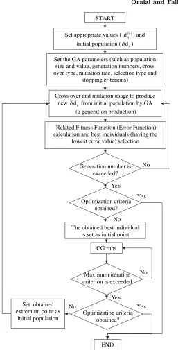
In all of this paper we use a hybrid optimization algorithm. This algorithm is the combination of the Genetic Algorithm and Conjugate Gradient (GA-CG). Since GA as an evolutionary algorithm is supposed to be a global optimization method, it does not heavily depend on the initial values of the variables. However, implementation of GA is very computer time consuming. On the other hand, CG is largely a local optimization method and its convergence to an extremum point depends on the initial values of variables. However, implementation of CG is relatively fast, but it requires the computation of gradients of functions. Consequently, combination of GA and CG may utilize the advantages of each one, avoiding the shortcomings of both. Therefore, the combined algorithm starts by implementing GA with a set of initial values for variables which leads towards an extremum. At about this point, GA is stopped and CG is activated to speed up the convergence towards a local extremum. Thereafter, the values of variables at this extremum point are taken as the initial values for GA. This algorithm is continued until the global extremum is arrived at. In all optimizations, the element positions are assumed to be as dn = d(0)n +δdn. Where
d(0)n is an appropriate value for the nth element position and δdn is its variation, which is calculated by the hybrid algorithm to meet the desired conditions. The complete flowchart of the GA-CG method is shown in Fig. 3.
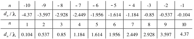
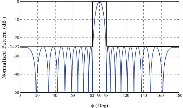
To illustrate the efficacy of the proposed method, a broadside pencil beam with 16 degree symmetrical beamwidth is designed for NUSLA with 20 elements. For this case, ϕF N = 98◦. The values of d(0)n are selected as the positions of elements in ESLA with 0.4λ spacings and the same number of elements. The hybrid algorithm finds optimum position of elements. The values of dn are listed in Table 1 and minimum achievableSLLis−24.87 dB. Also the optimum designed NUSLA’s pattern is shown in Fig. 4.
Table 1. Position of elements for optimum designed NUSLA (N = 20).
n -10 -9 -3 -2 -1
/ n
d -4.37 -3.597 -2.928 -2.449 -1.956 -1.614 -1.184 -0.85 -0.537 -0.104
n
/ n
d 0.104 0.537 0.85 1.184 1.614 1.956 2.449 2.928 3.597 4.37 λ
λ
1 2 3 4 5 6 7 8 9 10
8 7 6 5 4
- - - -
Set appropriate values ( (0 ) n
d ) and initial population ( d )n
Set the GA parameters (such as population size and value, generation numbers, cross over type, mutation rate, selection type and
stopping criterions) START
Optimization criteria obtained?
No Cross over and mutation usage to produce
new d from initial population by GA n
(a generation production)
Related Fitness Function (Error Function) calculation and best individuals (having the
lowest error value) selection
CG runs
Maximum iteration criterion is exceeded
Ye s
END
No
No Set obtained extremum point as
initial population
Generation number is exceeded?
Optimization criteria obtained?
No The obtained best individual
is set as initial point Ye s
Ye s Ye s
with simple feed network can generate a pattern similar to the Dolph-Chebychev pattern. Also, it is verified that the minimum SLL for a specified BW by the hybrid algorithm may be realized because the Dolph-Chebychev pattern has the minimumSLLfor a specified BW.
0 20 40 60 82 90 98 120 140 16 0 180
-50 -40 -30 -20 -10 0
-24.87
(Deg)
No
rm
a
li
zed
P
a
tt
ern
(d
B
)
φ
Figure 4. Pattern of designed NUSLA forBW = 16◦ and minimum achieved SLL=−24.78 dB.
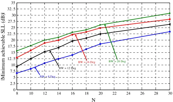
Although for the equally spaced linear array withN elements and spacing d, the Dolph-Chebychev excitation gives minimum SLL for a specified BW, but for nonuniformly spaced linear array, there is no similar relation for the element spacing. In fact, the main reason is due to the nonlinear relation between dn and E(ϕ). Here, for the first time, with the hybrid algorithm, for a specified BW and constant N, the minimum SLL is achieved for NUSLA. The results for N = 8,10,12,14,16,18,20,30 and BW = 8,12,16,20 degrees are drawn in Fig. 5.
As Fig. 5 shows, the minimum SLLfor constant N and specified
8 10 12 14 16 18 20 22 24 26 28 30 0
2.5 5 7.5 10 12. 5 15 17.5 20 22. 5 25 27.5 30 32. 5 35
N
|M
ini
m
u
m
a
ch
ie
v
a
b
le
S
L
L
(
d
B
)|
BW = 8 Deg
BW = 12 Deg
BW = 16 Deg BW = 20 Deg
Figure 5. (Minimum achievable SLL)-N curves with BW as parameter for NUSLA.
4. NUSLA DESIGN FOR SPECIFIED DIRECTIVITY AND SIDELOBE LEVEL
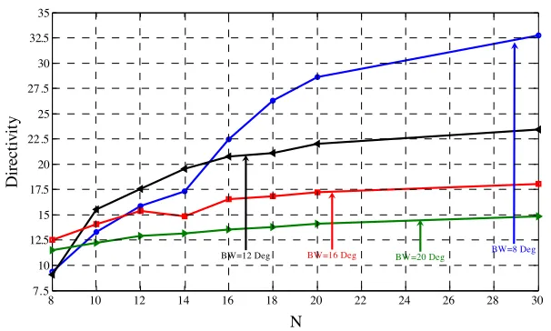
In Section 3, we designed for the minimumSLL and tightly specified beamwidth. However, sometimes designers may desire to design NUSLA for a specified directivity. The narrowest beamwidth may be judged as maximum directivity, but it is not always the case. When the array length of equally spaced linear array with mainbeam in
ϕ0 direction, increases (for constant N), beamwidth decreases and
directivity increases until the element spacing (d) exceeds λ/(1 + |cosϕ0|) and grating lobe appears [19]. With the grating lobe
appearance, the beamwidth still decreases but directivity falls so rapidly that the inverse relation betweenDand beamwidth is not true in this condition. For the broadside pattern (ϕ0 = 90◦), whendexceeds
1λ, this situation happens. But what happens for the nonuniformly spaced linear array in a similar condition? Before answering this question, we would like to show that the NUSLA design for a constant specifiedBW should not be interpreted as NUSLA design for constant
D.
4.1. Directivity and BeamwidthRelationship
8 10 12 14 16 18 20 22 24 26 28 30 7.5
10 12.5 15 17.5 20 22.5 25 27.5 30 32.5 35
N
Dire
ct
iv
it
y
BW=12 Deg BW=16 Deg BW=20 Deg BW=8 Deg
Figure 6. Directivity-N curves with BW as parameter for the designed NUSLA in Section 3 for the minimum SLL and tightly specifiedBW.
calculated by Eq. (7) and plotted in Fig. 6. In this figure,D is drawn versusN and BW is a parameter. As we expect, the directivity for a pattern with constant BW, is not constant and changes with N and spacing. Also, for instance, forBW = 8◦, when N is smaller than 16, the array directivity becomes smaller than the directivity of array with the same number of elements butBW = 12◦. These results showthat in the case of array pattern design for a specified directivity, sometimes
BW is not a good criterion.
Therefore, we propose the hybrid algorithm to design NUSLA with the specifiedD and bearableSLL.
Fitness function (error function) for this problem defined as:
errorD−SLL=errorD+errorSLL
errorD=|D−Ddesired|2 (15)
errorSLL=
|SLL(dB)−SLLthreshold(dB)|2
if SLL(dB)> SLLthreshold(dB)
0 else
whereDdesiredis the desired directivity andSLLthresholdis the bearable
SLLin dB.
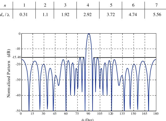
For example we design NUSLA with N = 14, Ddesired = 22 for
Then, the hybrid algorithm should solve the problem with the MAD
constraint according to:
|dn−dn±1|> M AD (16)
Here, we setM AD= 0.5λ. The hybrid algorithm solved this problem. The resultant directivity is 22.1 and SLL is−15.5 dB. The values ofdn are listed in Table 2. Because of symmetry, only positions of right side elements are listed. Also, the optimally designed NUSLA’s pattern is shown in Fig. 7.
Table 2. Position of right side elements for optimum designed NUSLA (N = 14).
n
/ n
d λ
1 2 3 4 5 6 7
0.31 1.1 1.92 2.92 3.72 4.74 5.56
0 15 30 45 60 75 90 105 120 135 150 165 180
-50 -40 -30 -20 -10 0
-15. 46
(Deg)
No
rm
a
li
zed
P
a
tt
er
n (
d
B
)
φ
Figure 7. Pattern of designed NUSLA (N = 14) with D= 22.1 and
SLL=−15.46 dB.
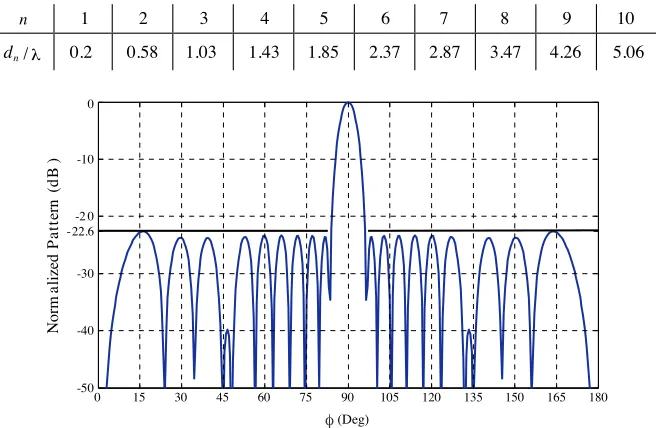
Table 3. Position of right side elements for optimum designed NUSLA (N = 20).
n
/ n
d λ
1 2 3 4 5 6 7 8 9 10
0.2 0.58 1.03 1.43 1.85 2.37 2.87 3.47 4.26 5.06
0 15 30 45 60 75 90 105 120 135 150 165 180
-50 -40 -30 -2 0 -10 0
-22.6
(Deg)
No
rm
a
li
zed
P
a
tt
ern
(d
B
)
φ
Figure 8. Pattern of designed NUSLA (N = 20) with D = 20 and
SLL=−22.6 dB.
It is necessary to mention that, there is a trade-off betweenDand
SLL. Whenever the desiredD is high, a lowSLLis difficult to obtain. We can enhance the value of directivity error or SLL error in Eq. (15) by weighting functions as follow:
errorD−SLL=WDerrorD+WSLLerrorSLL (17) where, WD and WSLL are the weights for directivity and SLL, respectively.
Therefore, with proper weighting, Eq. (17) may be used to design NUSLA for a desired D and bearable SLL or a desired SLL and thresholdD.
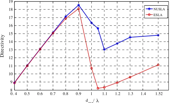
4.2. Directivity and LengthRelationship for NUSLA
and dave from Eq. (12) becomes wider. And then for each new length (or new dave), with the hybrid algorithm, the optimum NUSLA is designed to show a suitable directivity in comparison with ESLA with the same length and same number of elements.
Here, with the hybrid algorithm, for somedave, NUSLA is designed to satisfy some constraints as follows:
1. The whole length of NUSLA should be exactly equal to the specified value ((N−1)dave) as:
|dM −d−M|= (N−1)dave (18) 2. For dave/λ ≤ 0.5, M AD = dave and for dave/λ > 0.5,
M AD= 0.5λ.
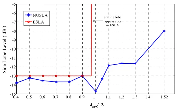
The desired directivity is specified to be as ESLA’s directivity (Dunif orm) for dave/λ ≤ 0.9 and bearable SLL equal to −13 dB. But for dave/λ > 0.9, that the grating lobe appears for ESLA and directivity falls rapidly, the NUSLA design purpose is reasonable SLL
and maximum achievable directivity. Therefore, Eq. (17) with suitable
WD and WSLL can be used as a fitness function. The elements of NUSLA are not necessary to be symmetrically located. Therefore, Eqs. (1) or (2) for E(ϕ) may be used. The hybrid algorithm found optimum NUSLA for some dave and N = 11. Their D and SLL are plotted in Figs. 9 and 10, respectively. Also, in these figures, the directivity andSLLof ESLA for element spacingdave and N = 11 are also shown. These results show that NUSLA for 1.4 > dave/λ >0.9 still results in good directivity and reasonable SLL.
0. 4 0.5 0.6 0.7 0.8 0.9 1 1.1 1.2 1.3 1.4 1.52
8 9 10 11 12 13 14 15 16 17 18 19
dav e/
Di
re
ct
iv
it
y
NUSLA
ESLA
λ
0.4 0.5 0.6 0.7 0.8 0.9 1 1.1 1.2 1.3 1.4 1.52 -15
-14 -13 -12 -11 -10 -9 -8 -7 -6 -5
d av e/
Side
L
ob
e
L
ev
el
(
dB
)
NUSLA ESLA
grat ing lobe ap pear ance in ESLA
λ
Figure 10. Comparison of SLL of ESLA and NUSLA having the same average element spacing forN = 11.
The pattern of optimum NUSLA for dave = 1.2λ and that of ESLA with the spacing dave = 1.2λbetween its elements is shown in Fig. 11. The element positions for NUSLA and ESLA are also shown in Fig. 12. As we can see, the minimum distance between elements is 0.68λand maximum distance is 2.77λto ensure the reduction of MC among elements.
5. NONUNIFORMLY SPACED PARALLEL DIPOLE ARRAY DESIGN
In this section, with the obtained results in Sections 3 and 4, the NUSLA with dipole elements will be designed.
5.1. Dipole Array Design for Specified BW and Minimum Achievable SLL
0 15 30 45 60 75 90 105 120 135 150 165 180 -25
-20 -15 -10 -5 0
-11.6
(Deg)
No
rm
al
ized
P
a
tt
ern
( d
B )
NUSLA ESLA
φ
Figure 11. Comparison of radiation pattern of ESLA and NUSLA fordave = 1.2λand N = 11.
-6 -4.8 -3.6 -2.4 -1.2 0 1.2 2.4 3.6 4.8 6
dn /
-5.19 -3.6 -0.83 -0.11 0.57 1.44 2.29 2.96 4.03
NUSLA
E SL A
-6 6
λ
Figure 12. Comparison of element positions in ESLA and NUSLA fordave = 1.2λand N = 11.
Table 4. Positions of right side elements for optimum designed parallel dipole array (N = 16).
n
/
n
d λ 0.252 0.793 1.436 1.992 2.616 3.44 4.272 5.134
1 2 3 4 5 6 7 8
The whole array pattern (Ew) is defined as:
Ew =E·Ee (19)
wavelength dipole shown in Fig. 2, defined as:
Ee= cos
π
2 cosθ
/sinθ (20)
The whole pattern of the designed parallel dipole array is drawn in the horizontal plane (θ = 90◦) in Fig. 13. As we expected, the element pattern does not change the first null position and SLLfrom those of the array factor.
0 15 30 45 60 75 849096 105 120 135 150 165 180
0
(Deg)
Normalized Horizontal Plane Pattern (dB)
Figure 13. The horizontal plane pattern of the designed parallel dipole array (N = 16, BW = 12◦).
5.2. Dipole Array Design for Specified Directivity and SLL
Consider the dipole array in Section 5.1 with N = 12. It is desired to have a pattern withDw = 25 (13.98 dBi) and minimum achievable
SLLwithSLLthreshold=−17 dB forM AD= 0.55λ.
We use the result of Section 4 and Eq. (8) to design the array factor with desired directivity. For half wavelength dipoles,De= 1.64.
Table 5. Position of right side elements for optimum designed parallel dipole array (N = 12).
n
/ n
d λ
1 2 3 4 5 6
The Eq. (8) gives D = Dw/De = 25/1.64 = 15.24, then with this desired directivity and Eq. (15), the hybrid algorithm will find the optimumdnfor symmetrical geometry. Because of symmetry only the right side element positions are listed in Table 5. The achieved D is 15.5 andSLL=−18.52 dB. The whole directivity is 25.42 (14.05 dBi). The whole directivity in the horizontal plane is drawn in Fig. 14.
0 15 30 45 60 75 90 105 120 135 150 165 180
0 5 10 14.05 15.27
(Deg)
Horizontal Plane Dir
ectivity (dBi)
Directivity (Eq. (8)) Directivity (Eq. (9)) Simulation (Feko)
Figure 14. The directivity of the designed parallel dipole array, calculated by Eq. (8), Eq. (9) and simulation.
This array is simulated by fullwave software, FEKO program [26]. For excitation, voltage sources with input impedances of 125 ohm are used. The directivity of simulated array in the horizontal plane is drawn in Fig. 14. As we can see, for the peak directivity atϕ= 90◦, there is 1.22 dBi difference between simulation and design values. This difference is due to the fact that Eq. (8) is an approximate formula. But it is acceptable. Also to showthe accuracy of Eq. (9), in comparison with Eq. (8), the directivity of the designed array, is calculated by Eq. (9) and plotted in Fig. 14. There is a good agreement between its results and simulation results. In Section 5.3, Eq. (9) will be used for the array design. It should be mentioned that MC causes the first sidelobe in the simulation results to become greater than our design value.
5.3. Dipole Array Design for Bearable Coupling Between Adjacent Elements
as some criteria to limit coupling among elements. But these criteria are not accurate enough. In [27–29], MC is defined. The coupling between two transmitter antennas is defined in [24] as:
C21=
P2
P1
= |S21|
2
1− |S11|2
(21) where P2 is the power received by antenna 2 and P1 is the power
delivered by antenna 1. This parameter is a better criterion than
MAD or dave. However, for NUSLA, the S-parameters computation for various distances among elements is a very cumbersome and time consuming problem. Since the array geometry is not kept fixed in the optimization process, the S-parameters should be computed in each run of GA-CG. On the other hand, the S-parameters computation is very difficult and their relations are scarce and imprecise. The array simulation by a fullwave simulator like IE3D is the best procedure, but by using the simulator for data generation for GA-CG, the CPU time may increase abruptly. To overcome this problem, we propose a NN-based model for the S-parameters estimation. Although NN is used for solving some various antenna problems [30–33], NN using for the calculation of S-parameters is proposed for the first time.
We propose a Radial Basis Function Neural Network (RBFNN) with three layers. For the training stage, we should generate the data with a fullwave simulator like IE3D. As a good approximation, only the adjacent element effects are included in the simulation. Since the maximum coupling occurs between two neighboring elements, we consider an array of three half wavelength dipoles with variable element spacing d1 and d2 as shown in Fig. 15 and simulate
it by IE3D at 3 GHz. Computed S-parameters are used for RBFNN training. The values of d1 and d2 are selected from the
set{10,20,30,40,50,60,70,80,90,100,110,120,130,160,200} all in mm. For instance, one possible case for (d1,d2) is (40 mm, 50 mm).
trained RBFNN has 255 neurons in the hidden layer and 6 neurons in output layer (real and imaginary parts of S-parameters are separately produced by RBFNN). This NN-based model is used by the hybrid optimization method. For instance, when the optimizer is to calculate
C24andC34, it gives (d24=|d2−d4|,d34=|d3−d4|) to RBFNN which
generates S44, S24 and S34 and then C24 and C34 by Eq. (21) can be
computed. Block diagram in Fig. 16 shows the proposed process.
d1 d2
Left adjacent Right adjacent
Figure 15. Three half wavelength dipoles with variable element spacingd1 and d2.
R BFN N
S- parameters : with two adjacent elements
Coupling with: R ight adjacent, L eft adjacen t d1
d2
Figure 16. S-parameters estimation by NN and computation of coupling with two adjacent elements.
Table 6. The optimum position of right side dipoles dn/λ obtained by GA-CG-NN.
n
/ n
d λ
1 2 3 4 5 6 7 8
0.26 0.74 1.25 1.73 2.25 2.75 3.35 4.28
Now, we can design NUSLA for a specified Cij between two adjacent elements. The fitness function (error function) is defined as:
errorD−SLL−C =WDerrorD+WSLLerrorSLL+WCerrorC (22) The first two terms on the right side are the same as Eq. (17) and
errorC shows the deviation from the bearable coupling and may be defined in various forms. WC is an enhancing coefficient, like WD and
Here, for parallel half wavelength dipole array withN = 16, it is desired to have SLL=−16 dB. Also, D is to be greater than 30 and |max(Cij)|>29 dB.
With these conditions, the optimization with GA-CG-NN method is performed. For the directivity computation, Eq. (9) which is accurate sufficiently was used. The optimum position of right side elements is listed in Table 6 andCij are listed in Table 7. The achieved peak directivity is 36.4 or 15.61 dBi and achieved SLL is −16.92 dB. Also, |max(Cij)| = 29.4 is achieved. The directivity in the θ = 90◦ plane (horizontal plane) is shown in Fig. 17.
This array is simulated by FEKO forf = 3 GHz with unit voltage sources with 125 ohm impedances as excitations. The simulation directivity in the horizontal plane is shown in Fig. 17. The peak directivity is D = 15.61 dBi or D = 36.4. The values of Cij derived from S-parameters by IE3D, are listed in Table 7 and compared with NN results. The value ofSLLis−16.5 dB. As we expected, by keeping coupling among elements belowa specified bearable value, its effect decreases. This is clearly seen by comparing Fig. 14 and Fig. 17 especially in the first sidelobe and mainbeam. The data reported in Table 7 verify the accuracy of the used RBFNN model for the calculation ofS-parameters and thenCij.
Table 7. Coupling in dB between each two adjacent elements of the optimized dipole array which is computed by NN model and IE3D.
n Cn,n-1(dB) (NN) Cn,n-1(dB) (Simulation) Cn,n+1(dB)(NN) Cn,n+1(dB)(Simulation)
0 15 30 45 60 75 90 105 120 135 150 165 180 -40
-35 -30 -25 -20 -15 -10 -5 0 5 10 20 15.61
-1.6
(Deg)
D
irect
iv
it
y
(
d
Bi
)
Directivity (Eq. (9)) Directivity (Simulation)
φ
Figure 17. Directivity of optimized NUSLA in the horizontal plane (θ= 90◦) from Eq. (9) and simulation in FEKO.
6. CONCLUSION
The obtained results showthe efficacy of the hybrid algorithm. These results are general and may be used for nonuniformly spaced linear array with arbitrary elements.
ACKNOWLEDGMENT
This work is supported in part by Iran Telecommunication Research Center (ITRC).
REFERENCES
1. Unz, H., “Linear arrays with orbitrarily distributed elements,”
IRE Trans. Antennas Propagat., Vol. 8, 222–223, Mar. 1960. 2. Skolnik, M. I., J. W. Sherman III, and G. Nemhauser, “Dynamic
programming applied to unequally spaced arrays,” IEEE Trans. Antennas Propagat., Vol. 12, 35–43, Jan. 1964.
3. Mailloux, R. J. and E. Cohen, “Statistically thinned arrays with quantized element weights,” IEEE Trans. Antennas Propagat., Vol. 39, 436–447, Apr. 1991.
4. Haupt, R. L., “Thinned arrays using genetic algorithms,” IEEE Trans. Antennas Propagat., Vol. 42, No. 7, 993–999, July 1994. 5. Donelli, M., S. Caorsi, and F. DeNatale, M. Pastorino, and
A. Massa, “Linear antenna synthesis with a hybrid genetic algorithm,” Progress In Electromagnetics Research, PIER 49, 1– 22, 2004.
6. Mahanti, G. K., N. Pathak, and P. Mahanti, “Synthesis of thinned linear antenna arrays with fixed sidelobe level using real coded genetic algorithm,”Progress In Electromagnetics Research, PIER 75, 319–328, 2007.
7. Meijer, C. A., “Simulated annealing in the design of thinned arrays having lowsidelobe levels,” Proc. South African Symp. Communication and Signal Processing, 361–366, 1998.
8. Razavi, C. A. and K. Forooraghi, “Thinned arrays using pattern search algorithms,” Progress In Electromagnetics Research, PIER 78, 61–71, 2008.
11. Ishimaru, A., “Theory of unequally-spaced arrays,” IRE Trans. Antennas Propagat., Vol. 10, 691–702, Nov. 1962.
12. Kumar, B. P. and G. R. Branner, “Design of unequally spaced arrays for performance improvement,” IEEE Trans. Antennas Propagat., Vol. 47, No. 3, 511–523, Mar. 1999.
13. Kumar, B. P. and G. R. Branner, “Generalized analytical technique for the synthesis of unequally spaced arrays with linear, planar, cylendrical or spherical geometry,”IEEE Trans. Antennas Propagat., Vol. 53, No. 2, 621–634, Feb. 2005.
14. Chen, K., Z. He, and C. Han, “A modified real GA for the sparse lineararray synthesis with multiple constraints,” IEEE Trans. Antennas Propagat., Vol. 54, No. 7, 2169–2173, July 2006. 15. Zhang, Y. F. and W. Cao, “Array pattern synthesis based on
weighted biorthogonal modes,” J. of Electromagn. Waves and Appl., Vol. 20, No. 10, 1367–1376, 2006.
16. Lee, K.-C. and J.-Y. Jhang, “Application of particle swarm algorithm to the optimization of unequally spaced antenna arrays,” J. of Electromagn. Waves and Appl., Vol. 20, No. 14, 2001–2012, 2006.
17. Ayestar´an, R. G., F. Las-Heras, and J. A. Mart´ınez, “Non uniform-antenna array synthesis using neural networks,” J. of Electromagn. Waves and Appl., Vol. 21, No. 8, 1001–1011, 2007. 18. Kazemi, S. and H. R. Hassani, “Performance improvement in
amplitude synthesis of unequally spaced array using least mean square method,”Progress In Electromagnetics Research B, Vol. 1, 135–145, 2008.
19. Stutzman, L. and G. A. Thiele,Antenna Theory and Design, 120– 121, John Wiley & Sons, 1998.
20. Bray, M. G., D. H. Werner, D. W. Boeringer, and D. W. Machuga, “Optimization of thinned aperiodic linear phased arrays using genetic algorithms to reduce grating lobes during scanning,”IEEE Trans. Antennas Propagat., Vol. 50, No. 12, 1732–1742, Dec. 2002. 21. Bray, M. G., D. H. Werner, D. W. Boeringer, and D. W. Machuga, “Thinned aperiodic, linear phased array optimizationfor reduced grating lobes during scanning with input impedance bounds,”
IEEE International Symposium on Antennas and Propagation Digest, Vol. 3, 688–691, Boston, MA, July 2001.
23. DeLuccia, C. S. and D. H. Werner, “Nature-based design of aperiodic linear arrays with broadband elements using a combination of rapid neural network estimation techniques and genetic algorithms,” IEEE Antennas and Propagation Magazine, Vol. 49, No. 5, 13–23, Oct. 2007.
24. Daniel, J. P., “Mutual coupling between antennas for emission or reception-application to passive and active dipoles,”IEEE Trans. Antennas Propagat., Vol. 22, No. 2, 347–349, 1973.
25. Taylor, T. T., “Design of line-source antennas for narrowbeam width and low side lobes,”IRE Trans. Antenna Propagat., Vol. 3, 16–28, 1955.
26. FEKO 5.2, www.feko.info
27. Zhu, Y.-Z., Y.-J. Xie, Z.-Y. Lei, and T. Dang, “Array a novel method of mutual coupling matching for array antenna design,”
J. of Electromagn. Waves and Appl., Vol. 21, No. 8, 1013–1024, 2007.
28. Zhou, Q., Y. J. Xie, and Z. Chen, “Prediction of equipment-to-equipment coupling through antennas mounted on an aircraft,”J. of Electromagn. Waves and Appl., Vol. 21, No. 5, 653–663, 2007. 29. Ayestaran, R. G., F. Las-Heras, and L. F. Herran, “High-accuracy
neural-network-based array synthesis including element coupling,”
IEEE Antennas and Wireless Propagation Letters, Vol. 5, 45–48, 2006.
30. Mohamed, M. D. A., E. A. Soliman, and M. A. El-Gamal, “Optimization and characterization of electromagnetically coupled patch antennas using RBF neural networks,” J. of Electromagn. Waves and Appl., Vol. 20, No. 8, 1101–1114, 2006. 31. Guney, K., C. Yildiz, S. Kaya, and M. Turkmen, “Artificial
neural networks for calculating the characteristic impedance of air-suspended trapezoidal and rectangular-shaped microshield lines,”
J. of Electromagn. Waves and Appl., Vol. 20, No. 9, 1161–1174, 2006.