A
p
-Variable Higher-Order Finite Volume Time Domain Method
for Electromagnetic Scattering
Avijit Chatterjee* and Subodh Joshi
Abstract—A higher-order accurate solution to electromagnetic scattering problems is obtained at reduced computational cost in a p-variable finite volume time domain method in a scattered field formulation. Spatial operators of lower order, including first-order accuracy, are employed locally in substantial parts of the computational domain during the solution process. The use of computationally cheaper and lower order spatial operators does not affect the overall higher-order accuracy of the solution. The order of the spatial operator at a candidate cell during numerical simulation can vary in space and time and is dynamically chosen based on an order of magnitude comparison of scattered and incident fields at the cell centre. Numerical results are presented for electromagnetic scattering from perfectly conducting two-dimensional scatterers subject to transverse magnetic and transverse electric illumination.
1. INTRODUCTION
Numerical simulation of electromagnetic (EM) scattering problems with full wave solvers in time domain like Finite Difference Time Domain (FDTD) or Finite Volume Time Domain (FVTD) method can result in long simulation times. This is especially true while dealing with large electrical sizes (a/λ1) where
a is the characteristic size or with scatterers containing cavities and intakes. A major contributor to large simulation time is the requirement of small mesh sizes to adequately resolve spatial phenomenon. Mesh sizes are usually dictated by points-per-wavelength (PPW) criteria which may be heuristic in nature. Higher-order spatially accurate schemes are able to resolve spatial variations with lower PPW in the computational domain than lower order representations. Higher-order spatially accurate methods can achieve similar accuracy levels on much coarser discretization than lower-order methods. However, higher-order spatially accurate methods tend to be more expensive on a per-grid-point basis than lower order counterparts which mitigates some of the advantages accruing from the use of coarser meshes. Thus, there is significant motivation in developing computationally low cost higher-order numerical methods for solving the time-domain Maxwell’s equations.
Multigrid (MG) methods [1, 2] based on cycling the numerical solution through a hierarchy of approximations either in space (h) or in polynomial order (p) or a combination of both have been used commonly to accelerate convergence to steady state of boundary value problems. h-MG methods are common in both finite volume and finite element frameworks while p-MG methods tend to be mostly restricted to mostly finite element framework [3]. Localh orprefinements have long been used, including for solving initial value problems, if the length scales to be resolved are not uniform across the computational domain and can cut down significantly on total computational time [4, 5]. Local refinement in the polynomial order (p) is again mostly restricted to finite element discretizations. A finite volume based solution of linear hyperbolic PDEs, including time-domain Maxwell’s equations,
Received 8 November 2017, Accepted 2 February 2018, Scheduled 9 February 2018
* Corresponding author: Avijit Chatterjee ([email protected]).
by cycling through successive lower orderp-approximations while retaining highest-order accuracy was proposed in [6, 7].
In the current work we propose ap-variable finite volume framework with an emphasis on solving EM scattering problems in the time domain. In the proposed framework, the time domain Maxwell equations which form a set of coupled linear hyperbolic PDEs, involving scattered field variables, are solved on a fixed grid but with the spatial operator formally varying in accuracy over the computational domain. The harmonic steady state solution obtained retains desired higher-order accuracy in spite of significant and not fixed parts of computational domain, processed using spatial operators of lower including first-order accuracy, during the simulation. The choice of accuracy of the spatial operator, done dynamically, is based on an order of magnitude comparison between the scattered and incident field at the cell center which serves as the measure of the local vertical scaling of the scattered field variable compared to the incident field. The framework requires an unified access to spatial operators of various orders of accuracy. For the present work the Essentially Non-Oscillatory (ENO) [8, 9] methodology is used to locally obtain spatial operators of the desired accuracy, but it would be possible to use any higher-order numerical method for solving linear hyperbolic PDEs that similarly provides unified access to spatial operators of varying accuracy. Numerical results are presented for EM scattering from perfectly conducting circular cylinder and airfoil.
2. P-VARIABLE HIGHER-ORDER ACCURACY
Consider the scalar advection equation to be the scalar representation of the time-domain Maxwell’s equations in differential form in a scattering process. The scalar advection equation for the scattered field is written as
∂u
∂t +c
∂u
∂x = 0 (1)
with wave speedc≥0. We assume u to represent a scattered field variable with
U =Ui+u (2)
where U and Ui respectively represent the corresponding total and incident fields. All variables in
Equation (1) can be nondimensionalized as u∗ = u/Ui, x∗ = x/λ and t∗ = t/T. λ and T are the
wavelength and time period for the harmonic incident wave. Further all nondimensional values u∗, x∗
and t∗ lie in [0,1] and in terms of order of magnitude are assumed to be O(1). Equation (1) can be written in corresponding nondimensional form as
∂u∗
∂t∗ +
∂u∗
∂x∗ = 0. (3)
The proposed p-variable method utilizes spatial operators of formally different orders of accuracy (p ≤ m) depending on the order of magnitude by which the local scattered field u(x, t) has been vertically scaled but always retains a local truncation error corresponding to the the highestmth order accuracy. Spatial operators of mand (m−1)th order formal accuracy result in local truncation errors of similar magnitude when being applied respectively to scattered field function with vertical scaling that differ by one-order-of-magnitude. This fact can be used recursively to involve even lower order operators while retaining formalmth order accuracy. We show this using the nondimensional form and an order-of-magnitude analysis of the local truncation error.
Consider the scattered field function u∗(x, t), discretization of the space derivative in Equation (3) with anmthorder accurate spatial operator results in a truncation error with leading term given by [10]
a(x∗)m∂
m+1u∗
∂m+1x∗ (4)
where ais a rational number. In a practical finite difference type formulation approximately 10 PPW or more would be required for a reasonable resolution for EM scattering problems which makes x∗ at least one order of magnitude less than the representative wavelengthλ. Thus,x∗ ∼O(1/10) in terms of order of magnitude. We now consider a scattered field functionv∗(x, t) obtained by vertically scaling
u∗(x, t) such that
Discretizing the space derivative in the nondimensionalized advection equation forv∗(x, t) given by
∂v∗
∂t∗ +
∂v∗
∂x∗ = 0, (6)
with an (m−1)th order accurate spatial operator will similarly lead to a truncation error with leading term
b(x∗)m−1∂
mv∗
∂mx∗ ∼b(x
∗)m−1∂mx∗u∗
∂mx∗ . (7)
For vertical scaling by constant Δx∗,
∂mx∗u∗
∂mx∗ ∼ x
∗∂mu∗
∂mx∗ (8)
is valid, using which Equation (7) can be rewritten as
b(x∗)m−1∂
mx∗u∗
∂mx∗ ∼b(x
∗)m∂mu∗
∂mx∗. (9)
We assume
∂mu∗
∂mx∗ =
∂m+1u∗
∂m+1x∗ =O(1) (10)
sinceu∗ and x∗ are bothO(1) in the nondimensionalization process. This is similar to fluid mechanics boundary layer theory, where the nondimensional velocity and distance in the streamwise direction are both O(1), resulting in the first and second derivatives of the streamwise velocity in the streamwise direction also beingO(1) [11]. Thus,
b(x∗)m−1∂
mx∗u∗
∂mx∗ ∼b(x
∗)m∂m+1u∗
∂m+1x∗. (11)
This implies the leading term of the truncation error resulting from spatial operators of the mth and (m−1)th accuracy given respectively in Equations (4) and (7) to be of comparable magnitude, i.e.,
a(x∗)m∂
m+1u∗
∂m+1x∗ ∼b(x∗)m−
1∂mv∗
∂mx∗. (12)
This can be applied recursively to bring in spatial operators of even lower order of accuracy while locally yielding spatial accuracy comparable to the highest mth order accuracy. Based on this a p -variable algorithm can be constructed to obtain inexpensively a spatially higher-order accurate steady state solution for a scattering process. The algorithm for the mth order accuracy in a cell centered Finite Volume Time Domain (FVTD) framework can be of the form described below and can be easily included in an existing higher-order solver for EM scattering problems,
• If the cell centered scattered variableu(xj, tk)≥ x×Ui(xj, tk) the spatial operator is of orderm.
xj,tk respectively represent discrete space and time.
• For cell centered variablexn+2×U
i(xj, tk)≤u(xj, tk)<xn+1×Ui(xj, tk) the spatial operator
is of order m−(n+ 1) with n≥0
withUi(x, t) assumed to be of similar order of magnitude throughout the domain andxn×Ui(xj, tk)∼
Ui(xj, tk)/10n.
The above algorithm is used to cheaply obtain higher-order accurate solutions to EM scattering problems in an FVTD framework. A method of lines approach decouples the time and space discretizations, and the spatial discretization is obtained using an Essentially Non-Oscillatory (ENO) method which allows easy access to varying orders of spatial accuracy. The current implementation is in the ENO-Roe form [8, 9], which efficiently implements the ENO reconstruction based on the numerical fluxes instead of the cell averaged state variables and is described for the scalar law. Equation (1) is written as a scalar hyperbolic conservation law
ut+f(u)x = 0, (13)
has the spatial derivative at theith grid point approximated as
∂f(u)
∂x |i=
1
x(fi+1/2−fi−1/2) +O(x
wherexis the grid size,pthe order of the scheme, andfi+1/2 the numerical flux function at the right
cell-face. Therth order accurate reconstruction of the numerical flux in the ENO scheme is
fi+1/2 =
r−1
l=0
αrk,lfi−r+1+k+l (15)
whereαrk,l are the reconstruction coefficients, andkis the stencil index selected among ther candidate stencils. The stencil Sk can be written as
Sk= (xi+k−r+1, xi+k−r+2, . . . , xi+k) (16)
and is locally the smoothest possible stencil. Details regarding reconstruction coefficients and stencil selection for ENO schemes are easily available in literature including [8, 9]. Extension to the multidimensional system of equations like the time-domain Maxwell’s equations can be obtained by decoupling the system into three scalar hyperbolic conservation laws normal to the cell faces [6, 12, 13]. The time domain Maxwell’s equations for transverse magnetic (TM) or transverse electric (TE) waves are written in a conservative form [12]
∂u
∂t +
∂f(u)
∂x +
∂g(u)
∂y =s. (17)
The vectors in Equation (17) for the TM waves are
u= Bx By Dz
, f=
0
−Dz/ε −By/μ
, g=
Dz/ε
0
Bx/μ
s=
0 0
−Jiz
(18)
while that for the TE waves are
u= Bz Dx Dy
, f=
Dy/ε
0
Bz/μ
, g=
−
Dx/ε
−Bz/μ
0
s= 0
−Jix −Jiy
. (19)
whereB is the magnetic induction,E the electric field vector,D the electric field displacement, Hthe magnetic field vector, and Ji the impressed current density vector, D = εE, B = μH with ε and μ
respectively the permittivity and permeability in free space. The FVTD method solves the conservative Maxwell’s equation in the integral form. Here a scattered field formulation is employed with the incident field assumed to be a solution of the Maxwell’s equations in free space and scattered field variables solved for. Integrating the differential form of the conservation law, represented by Equation (17), in the absence of a source term over an arbitrary control volume Ω
∂ΩudV
∂t +
Ω
∇.(F(u))dV = 0. (20)
F is the flux vector with components f, g in the Cartesian x, y directions. The integral form of the conservation law to be discretized is obtained by applying the divergence theorem as
∂ΩudV
∂t +
SF(u).nˆdS = 0 (21)
with nˆ the outward unit normal vector. The spatially discretized form solved for in a scattered and cell-centered formulation in the present work is finally written as [12]
Akduk
dt +
4
j=1
[(F(u).nˆS)j]k= 0 (22)
where the numerical flux [(F(u).nˆS)j]k approximates the average flux through facej of cellk, andAk
3. NUMERICAL RESULTS
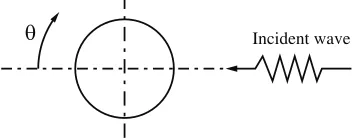
Numerical results are presented for EM scattering from 2D perfectly conducting circular cylinders as shown in Figure 1 and compared with the exact solution. A body confirming “O” mesh defines the computational domain with PEC boundary conditions on the cylinder surface and characteristic based far-field conditions at the outer boundary. Results are presented for both TM and TE continuous harmonic incident fields. Computations are performed for a fixed set of time periods of the incident harmonic wave, after which complex surface currents are obtained using a Fourier transform. The bistatic Radar Cross Section (RCS) or scattering width is then computed using a far-field transformation [14]. A discussion on the number of incident wave periods to be time-stepped for attaining sinusoidal steady state in a FDTD framework under harmonic incident excitation as attempted here is presented in [15]. The first problem considered is that of the circular cylinder subject to continuous harmonic incident TM illumination with a/λ = 4.8 where a is the cylinder radius and
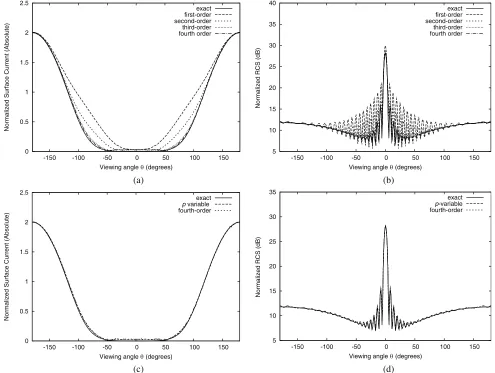
λ the wavelength of the incident wave [6, 12, 16]. Results are shown in terms of bistatic RCS and the absolute value of surface current after time stepping fixed incident time periods usually adequate for desired steady state response in such problems. Figures 2(a) and 2(b) show sample results for a conventional implementation for different spatial orders of accuracy on an “O” grid with 300 points in the circumferential direction corresponding to a resolution of 10 PPW on the scatterer surface after 5 time periods. The number of points in the radial direction is always kept constant at 50. A relatively lower resolution of 10 PPW on the cylinder surface is deliberately chosen to bring out the effect of the numerical discretization error on the solution obtained using different spatial orders of accuracy from the fourth to first. As expected, the highest fourth-order accurate solutions are closest to the exact solution with the first and second-order accurate solutions showing significant deviation away from near-specular-regions. The monostatic point is located at ±180◦ in the bistatic plot with 0◦ the perfect shadow. The same problem is now solved with a p-variable method with m = 4. An order of magnitude comparison of scattered and incident cellwise value of Dz is used to fix the local (cellwise)
order of accuracy (p≤4) of the spatial operator.
Incident wave θ
Figure 1. Schematic of a circular cylinder illuminated with an incident field.
Results are presented after 5 time periods in Figures 2(c) and 2(d) and compared with exact and conventional fourth-order results. Results from p-variable method with m = 4 match closely with conventional fourth-order results. L1,L2 andL∞norms of relative error for surface current density and
bistatic RCS are tabulated in Table 1. It can be seen that thep-variable method shows similar relative errors to the conventional fourth-order ENO scheme.
0 0.5 1 1.5 2 2.5
-150 -100 -50 0 50 100 150
Normalized Surface Current (Absolute)
Viewing angle θ (degrees)
exact first-order second-order third-order fourth order
5 10 15 20 25 30 35 40
-150 -100 -50 0 50 100 150
Normalized RCS (dB)
Viewing angle θ (degrees)
exact first-order second-order third-order fourth order
0 0.5 1 1.5 2 2.5
-150 -100 -50 0 50 100 150
Normalized Surface Current (Absolute)
Viewing angle θ (degrees)
exact p variable fourth-order
5 10 15 20 25 30 35
-150 -100 -50 0 50 100 150
Normalized RCS (dB)
Viewing angle θ (degrees)
exact p-variable fourth-order
(a) (b)
(c) (d)
Figure 2. Bistatic RCS and surface current densitya/λ= 4.8, continuous harmonic TM illumination,
p-variable and conventional. (a) Surface current density. (b) Bistatic RCS. (c) Surface current density. (d) Bistatic RCS.
Table 1. Relative error norms for different numerical schemes including the p-variable method for bistatic RCS and surface current density in TM case.
Bistatic RCS
Schemes O(1) O(2) ENO O(3) ENO O(4) ENO p-variable
L1 Error 1.54E-01 7.05E-02 2.12E-02 1.26E-02 1.28E-02
L2 Error 2.52E-01 1.24E-01 3.36E-02 1.70E-02 1.73E-02
L∞Error 3.89E-01 2.19E-01 6.28E-02 2.84E-02 2.94E-02 Surface Current Density
L1 Error 2.77E-01 1.09E-01 3.27E-02 2.02E-02 2.23E-02
L2 Error 2.50E-01 1.03E-01 2.64E-02 1.65E-02 1.79E-02
-20 -10 0 10 20 30 40
-150 -100 -50 0 50 100 150
Normalized RCS (dB)
Viewing angle θ (degrees)
exact first-order second-order third-order fourth order
-5 0 5 10 15 20 25 30 35 40
-150 -100 -50 0 50 100 150
Normalized RCS (dB)
Viewing angle θ (degrees)
exact p-variable fourth-order
(a) (b)
Figure 3. Bistatic RCS a/λ = 9.6, continuous harmonic TE illumination. (a) Conventional (b)
p-variable.
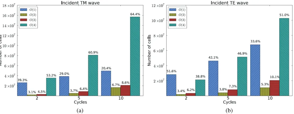
(a) (b)
Figure 4. Computational work distribution forp-variable method. (a) TM case. (b) TE case.
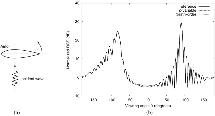
We also consider scattering from a perfectly conducting NACA 0012 airfoil as shown in Figure 5(a). The airfoil chord length is 10 times the wavelength of the incident harmonic TM wave at broadside incidence [6, 12, 16]. Results are obtained using a body-fitted “O” grid with 200 points around the airfoil and 50 in the normal direction. Figure 6 compares RCS results after 5 time periods using regular fourth-order spatial accuracy and p-variable fourth-order (m = 4). Both results are compared with a “reference solution” obtained using regular fourth-order spatial accuracy but on a much finer grid with 1600 points around the airfoil and time stepped for 10 time periods. Again, like in the case of the circular cylinder an almost exact match is obtained between the conventional andp-variable method of the same formal accuracy. Figure 6 lists the percentage of the computational domain over time processed by spatial operatorsp≤4. The trend is similar to that for scattering from perfectly conducting circular cylinders.
Incident wave Airfoil
-10 0 10 20 30 40
-150 -100 -50 0 50 100 150
Normalized RCS (dB)
Viewing angle θ (degrees)
reference p-variable fourth-order
θ
(a) (b)
Figure 5. Bistatic RCSa/λ= 10, continuous harmonic TM illumination,p-variable and conventional. (a) NACA 0012 airfoil schematic. (b) Bistatic RCS.
Figure 6. Computational work distribution forp-variable method; airfoil case.
Table 2. Saving in computing time withp-variable method (m= 4).
Computational Performance — Work Units
TM Case TE Case
Cycles Conventional p-variable % Conventional p-variable %
O(4) Method Saving O(4) Method Saving 2 4.52e08 2.84e08 37.24 3.72e08 1.91e08 48.62 5 9.04e08 6.36e08 29.62 7.47e08 4.40e08 41.11 10 1.66e09 1.24e09 25.14 1.37e09 8.78e08 35.96
method with m= 4, total computing cost (Ctotal) can then be written as,
Ctotal=
4
p=1
where, Cp is the computational cost per-cell atpth level andnp the total number of cells processed at
pth level. On the other hand, the uniformly 4th-order accurate scheme will incur a cost of (nTC4) work
units, wherenT is the total number of cells on the domain. The variation in computing cost with order
of accuracy for a 2D FV ENO scheme is seen to follow C3 = 2.2C2 and C4 = 3.4C2 [17]. Assuming
C2= 2C1, we getC2/C1 = 2, C3/C1 = 4.4 andC4/C1 = 6.8. Table 2 shows the saving in computational
cost over conventional fourth-order method in terms of work units assumingC1 = 1 unit for test cases
involving circular cylinders. A similar calculation yields a saving of 43.4% for the test case of NACA 0012 airfoil.
4. CONCLUSION
Desired higher-order spatial accuracy can be maintained, while using lower-order spatial operators in substantial parts of the computational domain in ap-variable FVTD method for solving EM scattering problems. Lower-order spatial operators come at much reduced computational cost and can cut down considerably on simulation time while retaining desired higher-order accuracy using the present method. An order of magnitude comparison of scattered and incident cell-centered EM field variables is used to decide on the local order of accuracy of the spatial operator. The local spatial order of accuracy can vary in space and time, and the proposed method can be easily integrated with existing higher-order FVTD techniques. The current implementation uses the ENO family to access spatial operators of desired order of accuracy as dictated by the order of magnitude comparison. Results are presented for the canonical case of EM scattering from a perfectly conducting circular cylinder as well as that of an airfoil.
REFERENCES
1. Brandt, A., “Multi-level adaptive solutions to boundary value problems,” Math. Comp., Vol. 31, 333–390, 1977.
2. Brandt, A., “Guide to multigrid development,” Multigrid Methods, W. Hackbusch, U. Trottenberg (Eds.), 220–312, Springer-Verlag, 1982.
3. Fidkowski, K. J., T. A. Oliver, J. Lu, and D. L. Darmofal, “p-multigrid solution of high-order discontinuous Galerkin discretizations of the compressible Navier Stokes equations,” J. Comp. Phys., Vol. 207, 92–113, 2005.
4. Berger, M. J. and J. Oliger, “Adaptive mesh refinement for hyperbolic partial differential equations,” J. Comp. Phys., Vol. 53, 484–512, 1984.
5. Babuˇska, I., “The p- and hp-versions of the finite element method: The state of the art,” Finite Elements: Theory and Applications, Springer, New York, 1988.
6. Chatterjee, A., “A Multilevel numerical approach with application in time-domain electromagnet-ics,”Commn. Comp. Phys., Vol. 17, 703–720, 2015.
7. Joshi, S. M. and A. Chatterjee, “Higher-order multilevel framework for ADER scheme in computational aeroacoustics,” J. Comp. Phys., Vol. 338, 388–404, 2017.
8. Shu, C. W. and S. Osher, “ Efficient implementation of essentially non-oscillatory shock-capturing schemes,”J. Comp. Phys., Vol. 77, 439–471, 1988.
9. Shu, C. W. and S. Osher, “Efficient implementation of essentially non-oscillatory shock-capturing schemes II,”J. Comp. Phys., Vol. 83, 32–78, 1989.
10. LeVeque, R. J., Finite Volume Methods for Hyperbolic Problems, Cambridge Texts in Applied Mathematics, Cambridge University Press, Cambridge, New York, 2002.
11. Kundu, P. K., I. M. Cohen, and D. R. Dowling, Fluid Mechanics, 5th Edition, Academic Press, Elsevier, Boston, 2015.
13. Chatterjee, A. and A. Shrimal, “Essentially nonoscillatory finite volume scheme for electromagnetic scattering by thin dielectric coatings,”AIAA J., Vol. 42, 361–365, 2004.
14. Balanis, C. A.,Advanced Engineering Electromagnetics, 2nd Edition, John Wiley, New York, 1989. 15. Taflove, A. and K. R. Umashankar, “Review of FD-TD numerical modeling of electromagnetic
wave scattering and radar cross section,” Proc. of the IEEE, Vol. 77, 682–699, 1989.
16. Deore, N. and A. Chatterjee, “A cell-vertex based multigrid solution of the time domain Maxwell’s equations,” Progress In Electromagnetics Research B, Vol. 23, 181–197, 2010.