Synthesis of MIMO System with Scattering Using Binary Whale
Optimization Algorithm with Crossover Operator
Pengliang Yuan*, Chenjiang Guo, and Qi Zheng
Abstract—In a MIMO system, scattering is always an important problem since it is closely related to the channel capacity of system. In most of previous works, scattering was usually neglected so as to simplify the process of analysis. Therefore, it is really necessary to investigate and understand the scattering effect on capacity. To this end, scattering is taken into consideration in terms of channel capacity in this paper. From the antenna point of view, antenna element layout can be viewed as an optimization problem. To resolve this problem, a binary whale optimization algorithm (BWOA) is proposed. We investigate the effect of scattering environment on the capacity of a MIMO system and make comparison with an existing method in performance. The simulated results demonstrate that the nonuniform sampling method is able to efficiently improve the capacity of system even for poor scattering environment.
1. INTRODUCTION
MIMO system can improve the performance of a system with spatial diversity or multiplexing [1, 2]. The fulfillment of multiplexing is very closely related to the low correlation characteristic of transmitting signals. The low correlation characteristic can be obtained with sampling strategy [3, 4].
Generally, a rich scattering environment widely adopts uniform distribution sampling by λ/2 spacing, while in a poor scattering environment, uniform distribution sampling will cause the problem of over-sampling. A poor scattering environment thus requires more sampling than λ/2. Presently, there are some methods available in literature for overcoming such a problem. These methods may be divided into two classes. One is adaptive sampling implemented by the technique of antenna selection [5] or controlled parasitic elements [6, 7], and the other is nonuniform sparse array arrangements [8]. Because the channel capacity of a MIMO system is closely associated with the scattering environment, antenna array system and position of elements, over the past few years, some evolutionary algorithms have also been applied to the optimization of capacity of MIMO systems, such as hybrid Genetic-Taguchi algorithm [9], Galaxy-based search algorithm [10], and spiral optimization technique [11]. Herein we optimize the antenna layout with binary whale optimization (BIWO) algorithm, based on an efficient algorithm, the whale optimization algorithm.
2. SYSTEM MODEL AND PROBLEM FORMULATION
Consider a narrow-band MIMO system, which consists of Nt transmitter and Nr receiver antennas. Assume that X ∈ CNt×1 represents the vector of transmit signals and that N ∈ CNr×1 denotes the
Received 20 June 2019, Accepted 16 August 2019, Scheduled 30 August 2019 * Corresponding author: Pengliang Yuan ([email protected]).
vector of additive noise at the receiver. Consequently, the received signals Y can be expressed in the form of a complex base-band notation as
Y=HX+N (1)
whereNis assumed to be an independent and uncorrelated noise vector, and uniformly distributed by zero mean and variance σ2 such that N(0, σ2INr), INr is a unitary vector. H ∈ CNr×Nt denotes the channel matrix of a MIMO system, which is represented as
H(k) ={hrt|r = 1,· · · , Nr; t= 1,· · · , Nt} (2)
where k represents the kth channel realization, k= 1,· · · , K. In the free space, the transfer function hrt from transmitter to receiver is derived by
hrt(d) =β λ 4πdexp
−j2πd
λ
(3)
where dis the distance between a pair of transmitter and receiver antennas. The loss in free space is given by λ/(4πd). β denotes the wavenumber,β = 2π/λ, where λdenotes the wavelength of the using carrier frequency. Provided that we take I random scattering points into consideration, the transfer functionhrt will be rewritten as
hrt(drt, drti) 1 2drt
exp (jβdrt) + I
i=1
1 2drti
exp (jβdrti) (4)
where the phase rotation caused by the propagation distance is introduced by complex exponential terms. drt is the distance between a pair of antenna elements, derived by
drt |Ri−Tj| (5)
whereRi andTj respectively stand for the position of theith receiver antenna and thejth transmitter antenna. In Eq. (4), drti is the distance via theith scattering point between a pair of antennas and can be defined as
drti|Ri−Sl|+|Sl−Tj| (6)
whereSl stands for the position of the lth scattering point. Whendrt anddrti are both known,H(k) is decomposed by means of singular value decomposition (SVD) [12].
H(k) =UΣV (7)
where U ∈ CNr×Nr, V ∈ CNt×Nt both stand for the unitary matrix and respectively contain the left and right singular vectors as toH. UandVare obtained by the eigenvalue decomposition of Hermitian matricesHHH and HHH. Σ∈CNr×Nt is a diagonal matrix with the positive singular values such that μ1,· · · , μn, where n= min{Nt, Nr} is the rank ofH. In the case of no channel state information, the capacityC(k) of the channels can be generally derived by
C(k)= n
i=1
log2
1 +P μi nσ2 n
bps/Hz (8)
whereP is the total transmitting power at transmitter.
Before allowing for the scattering environment, the elements layout needs to be given beforehand. The elements layout as an optimization problem is summarized as follows
find (Ri, Tj) = argmax C(k)
subject to |Ri−Ri−1| λ/2, i= 1,· · · , Nr
|Tj−Tj−1| λ/2, j= 1,· · · , Nt
(9)
3. BINARY WHALE OPTIMIZATION ALGORITHM (BWOA)
The whale optimization algorithm (WOA) as a nature-inspired algorithm exhibits unique features such as robustness and practical convenience [13]. Such advantages motivate us to resort to the WOA algorithm to solve the problem in Eq. (9). However, it is difficult to directly deal with the above mentioned problem in Eq. (9), because the original WOA algorithm is only able to solve the problem of real number variable. Consequently, we propose the binary WOA algorithm to solve binary problem. For such a problem, the crucial point is to map a continuous search space into discrete binary search space only including 0 and 1 as for the candidate solution. Here we prepare to exploit the transfer function to achieve the search space transformation. In addition, the crossover strategy is introduced to overcome the problem of updating the worst individual, which causes the low efficiency of WOA algorithm. For simplicity, only modified components are presented.
(i) Crossover strategy: For the ith individual to enforce the crossover operator, the ith and i−1th individuals are selected from the current population pool, then both of them take part in the crossover operation. The process can be formulated as
(ˆxi,xˆi−1) =(xi, xi−1) (10)
whereis an operator carrying out the crossover scheme between the two selected binary solutions only for the latter half of dimension. xi represents the ith individual at the tth iteration. Using Eq. (10) will produce two intermediate solutions in binary search space, and choosing which one of them as the final solution is determined by the random probabilityr. Its determinant criterion is written as the following
xi(new) =
ˆ
xi, r≥0.5 ˆ
xi−1, otherwise
(11)
(ii) Space transformation: For search space mapping, there are two families of transfer functions available, S-shaped and V-shaped transfer functions. Firstly, we use the S-shaped transfer function to obtain the probabilityp.
p(xij) = 1 1 + exp(−xi
j)
(12)
where xij is the ith individual in the jth dimension at the tth iteration. p(xij) is the output probability of individual xij. Next comparing p(xij) with a rand number obtains and updates the new position x, and the determined behavior can be written as
xij =
0 r < p(xij)
1 r ≥p(xij) (13)
where xij represents the i element at the j dimension in the candidate solution space at the dth iteration.
Algorithm 1 provides the pseudo code of the BWOA, and the corresponding parameters definition is given in Table 1. See [13] for more details of WOA. In summary, the entire design procedure is provided as follows.
(1) Initialization: GivenNr and Nt, the maximum iteration tmax equals 100, and setCopt= 0.
(2) Array design: Using BWOA produces the new elements layout. ComputeHand C(k).
(3) Update optimum capacity: Obtain the best fitnessf it from current population and compare f it withCopt. Iff itoutperformsCopt,Copt will be updated by the currentf it.
(4) Convergence check: When iteration times is greater than the giventmax, end iteration. Otherwise,
return (2).
Algorithm 1: Pseudo code of the BWOA
Input: input parameters t, tmax,l,r
Output: X∗
Initialize the whales populationXi(i= 1,2,· · ·, n) 1
Calculate the fitness of each search agent 2
X∗=the best search agent 3
whilet < tmax do 4
foreach search agent do
5
Updateα, A, C, l and p 6
if p <0.5 then
7
if |A| ≤1then
8
Update the position of the current search agent byD=|C·x∗(t)−X(t)| 9
X(t+ 1) =X∗(t)−A·D
else
10
Update the position of the current search agent by theD=|C·xrand−X(t)| 11
X(t+ 1) =xrand−A·D
else
12
Update the position of the current search agent by D =|X∗(t)−X(t)| 13
X(t+ 1) =D·ebl+ cos(2πl) +X(t)
Calculate the probabilities using a transfer function taking Eqs. (12) and (13) 14
Crossover operator between xi and xi−1 by Eqs. (10) and (11) 15
Calculate the fitness of each search agent 16
UpdateX∗ if there is a better solution 17
t=t+ 1 18
Table 1. Parameters specification.
Symbol Quantity Value
Algorithm 1
t iteration times [1,tmax] tmax maximum of iteration 100
b random number (0,10)
l random number (−1,1) A control parameter 2α·r−α C control parameter 2·r α control parameter 2(1−t/tmax)
r random number [0,1]
4. SIMULATION RESULTS
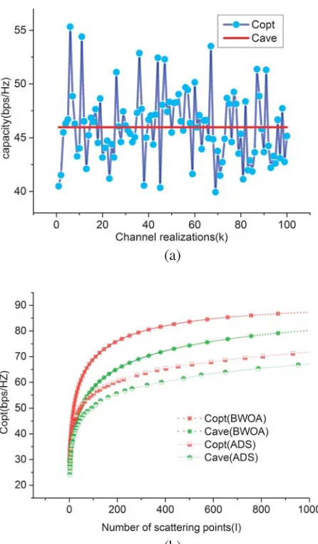
Herein considering a case, Nt=Nr = 5 and the power P = 1 W. The channel realization K is chosen to be 100, and the scattering point number I ∈[10,1000]. Assume that xri, xtj respectively denote the ith andjth element positions along x dimension at the receiver and transmitter.
(a)
(b)
Figure 1. The optimum capacity and average capacity for Nt =Nr = 5 under the optimum elements layout. (a) The resultant capacity and average capacity with channel realizations number (I = 10). (b) The resultant capacity Copt and average capacity Cave with scattering points number (k= 1).
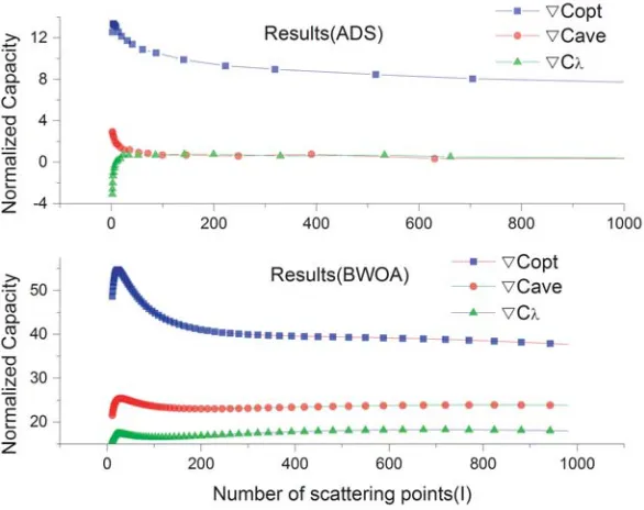
realization k and scattering points number I. In Fig. 1(a), the capacity and average capacity are provided with varying k∈ [1,100] when I = 10. The average capacity Cave = (Ki=1Copt)/K reaches 45.98 bps/Hz and is marked as a straight line in Fig. 1(a). As can be seen, there is an improvement of 15 bps/Hz in Cave in comparison with the almost difference sets (ADS) of the literature [8]. Fig. 1(b) depicts the relationship between the capacity and the number of scattering points with the BWOA and ADS. As can be seen, the proposed BWOA obtains a better normalized capacity than ADS. It demonstrates the effectiveness of the proposed BWOA for improving the capacity of system. When I varies from 10 to 1000, the corresponding normalized capacities obtained by BWOA and ADS are presented in Fig. 2, which includes the optimal capacity ∇Copt ( ¯Copt −C¯λ/2), average capacity
∇Cave ( ¯Cave −C¯λ/2), and capacity ∇Cλ ( ¯Cλ −C¯λ/2) with varying the uniform distribution by
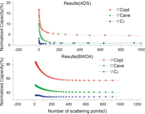
spacingλ, where ¯C= (ni=1C)/n(n= 1,· · · , I). As can be seen,Copt and Cave of BWOA outperform those of ADS. The convergence curve corresponding to Fig. 2 is presented in Fig. 3. As can be seen, BWOA is able to implement the fast convergence in a short iteration.
Figure 2. The normalized capacity vs number of scattering points (Nt=Nr= 5,k= 100).
Figure 3. The convergence curve of BWOA corresponding to Fig. 2 (Nt=Nr= 5, k= 100).
Figure 4. The normalized capacity vs number of scattering points (Nt=Nr= 15, k= 100).
Figure 5. The convergence curve of BWOA corresponding to Fig. 4 (Nt=Nr= 5, k= 100).
5. CONCLUSION
ACKNOWLEDGMENT
This work was supported in part by the Science Research Project of Gansu Province Higher Educational Institutions (grant No. 2019A-268), in part by the China Scholarship Council and the Excellent Doctorate Cultivating Foundation of Northwestern Polytechnical University.
REFERENCES
1. Goldsmith, A., S. A. Jafar, N. Jindal, and S. Vishwanath, “Capacity limits of MIMO channels,”
IEEE JSAC, Vol. 21, No. 5, 684–702, 2003.
2. Paulraj, A. J., D. A. Gore, R. U. Nabar, and H. Bolcskei, “An overview of MIMO communications — A key to gigabit wireless,” Proceedings of the IEEE, Vol. 92, No. 2, 198–218, 2004.
3. Migliore, M., “On the role of the number of degrees of freedom of the field in MIMO channels,”
IEEE Transactions on Antennas and Propagation, Vol. 54, No. 2, 620–628, 2006.
4. Gao, Y., A. J. H. Vinck, and T. Kaiser, “Massive MIMO antenna selection: Switching architectures, capacity bounds and optimal antenna selection algorithms,” IEEE Transactions on Signal Processing, Vol. 66, No. 5, 1346–1360, 2018.
5. Molisch, A. F. and M. Z. Win, “MIMO systems with antenna selection — An overview,” IEEE Microwave Magazine, Vol. 5, No. 1, 46–56, 2004.
6. Migliore, M. D., D. Pinchera, and F. Schettino, “Improving channel capacity using adaptive MIMO antennas,”IEEE Transactions on Antennas and Propagation, Vol. 54, No. 11, 3481–3489, 2006. 7. Pinchera, D., J. W. Wallace, M. D. Migliore, and M. A. Jensen, “Experimental analysis of a
wideband adaptive-MIMO antenna,” IEEE Transactions on Antennas and Propagation, Vol. 56, No. 3, 908–913, 2008.
8. Oliveri, G., F. Caramanica, M. Migliore, and A. Massa, “Synthesis of nonuniform MIMO arrays through combinatorial sets,” IEEE Antennas and Wireless Propagation Letters, Vol. 11, 728–731, 2012.
9. Recioui, A., “Capacity optimization of MIMO wireless communication systems using a hybrid genetic-taguchi algorithm,”Wireless Personal Communications, Vol. 71, No. 2, 1003–1019, 2013. 10. Recioui, A., “Application of a galaxy-based search algorithm to MIMO system capacity
optimization,” Arabian Journal for Science & Engineering, Vol. 41, No. 9, 3407–3414, 2016. 11. Recioui, A., “Application of the spiral optimization technique to antenna array design,”Handbook
of Research on Emergent Applications of Optimization Algorithms, IGI Global, 364–385, 2018. 12. Telatar, E., “Capacity of multi-antenna gaussian channels,” Transactions on Emerging
Telecommunications Technologies, Vol. 10, No. 6, 585–595, 1999.