1
Improving Monsoon Precipitation Prediction using Combined Convolutional 1
and Long Short Term Memory Neural Network 2
Qinghua Miao1, Baoxiang Pan2,*, Hao Wang1,3 3
Kuolin Hsu2, Soroosh Sorooshian2 4
1 State Key Laboratory of Hydroscience and Engineering, Department of Hydraulic 5
Engineering, Tsinghua University, Beijing, 100084, China 6
2 Center for Hydrometeorology and Remote Sensing, University of California, 7
Irvine, CA, 92617 8
3 Department of Water Resources, China Institute of Water Resources and 9
Hydropower Research, Beijing, 100038, China 10
11
Submitted to Water
12
13
*Corresponding author address:
14
Baoxiang Pan, Email: [email protected]
15
16
17
Abstract: 19
Precipitation downscaling is widely employed for enhancing the resolution and 20
accuracy of precipitation products from general circulation models (GCMs). In this 21
study, we propose a novel statistical downscaling method to foster GCMs’ precipitation 22
prediction resolution and accuracy for monsoon region. We develop a deep neural 23
network composed of convolution and Long Short Term Memory (LSTM) recurrent 24
module to estimate precipitation based on well-resolved atmospheric dynamical fields. 25
The proposed model is compared against GCM precipitation product and classical 26
downscaling methods in the Xiangjiang River Basin in South China. Results show 27
considerable improvement compared to the ECMWF-Interim reanalysis precipitation. 28
Also, the model outperforms benchmark downscaling approaches, including 1) quantile 29
mapping, 2) support vector machine, and 3) convolutional neural network. To test the 30
robustness of the model and its applicability in practical forecast, we apply the trained 31
network for precipitation prediction forced by retrospective forecasts from ECMWF 32
model. Compared to ECMWF precipitation forecast, our model makes better use of the 33
resolved dynamical field for more accurate precipitation prediction at lead time from 1 34
day up to 2 weeks. This superiority decreases along forecast lead time, as GCM’s skill 35
in predicting atmospheric dynamics being diminished by the chaotic effect. At last, we 36
build a distributed hydrological model and force it with different sources of 37
precipitation inputs. Hydrological simulation forced with the neural network 38
precipitation estimation shows significant advantage over simulation forced with the 39
the performance is just slightly worse than the observed precipitation forced simulation 41
(NSE=0.82). This further proves the value of the proposed downscaling method, and 42
suggests its potential for hydrological forecasts. 43
Key Words: Precipitation downscaling; Convolutional Neural Networks; Long Short 44
Term Memory Networks; Hydrological simulation 45
46
1. Introduction 47
Precipitation is a primary forcing in hydrological systems (Nijssen and Lettenmaier 48
2004). Obtaining accurate and reliable precipitation data at relevant spatial and 49
temporal scales is crucial for efficient water resources management and timely warning 50
of precipitation-related natural hazards, such as flood and drought. To sustain a 51
reasonably long lead-time for the above-mentioned applications, it is imperative to 52
employ precipitation prediction techniques. 53
For short-term range up to climate range, numerical weather/climate modeling is 54
perhaps the only reliable tool for predictions. Through the past decades, numerical 55
models have achieved impressive progresses in predicting atmospheric dynamics and 56
physics (Bauer et al., 2015). Here, dynamics refer to atmospheric state variables (i.e., 57
density, pressure, temperature, and velocity) that are explicitly described by 58
atmospheric primitive equations and resolved by numerical partial differential equation 59
solvers, while physics refer to the unresolved processes that are diagnosed from the 60
resolved variables based on empirical parameterization schemes. Precipitation results 61
satisfactory skills in resolving the atmospheric dynamics, models’ precipitation 63
estimation suffers from multiplicate sources of errors (Tapiador et al., 2018), and the 64
skill has been described as “dreadful” (Stephens et al., 2010). The uncertainties for 65
precipitation prediction generally stem from the following aspects: 1) models’ 66
dynamical forcings are of limited resolution for making detailed representation of cloud 67
microphysics; 2) we usually do not have direct observation for the initial distribution 68
state for cloud hydrometeors of liquid, solid, or mixed phases; 3) the evolution and 69
interaction of precipitating cloud hydrometeors are not well described, due to our 70
limited understandings or computation resources. Models’ deficiencies in each of the 71
above aspects quickly reveal themselves in the precipitation product (Tapiador et al., 72
2018). Many studies have revealed that the accuracy of the rainfall prediction in GCMs 73
(such as ECMWF and NCEP) is far from enough to be used directly in East Asian 74
monsoon region (Kang et al. 2002; Wang et al. 2004). Besides the “dreadful” effect, the 75
resolution of the computing grids is also usually too coarse for hydrological simulations 76
(Xu 1999; Ghosh, 2010; Meehl et al., 2007). 77
To improve the precipitation estimations of GCMs, hydrologists have developed 78
various downscaling methods, including the dynamical downscaling and statistical 79
downscaling (Benestad, 2007; Benestad and Haugen, 2007; Christensen et al. 1997, 80
2007; Hanssen et al. 2005; Prudhomme et al. 2002; Xu, 1999). Dynamical downscaling 81
usually includes running a regional climate model with the initial and boundary 82
conditions provided by GCMs. The massive computational cost and the requirement of 83
downscaling establishes statistical links between large scale weather and local 85
observation. Despite some limitations, such as the stationarity assumption in the 86
predictor–predictand relationship and requirement for long observation records, 87
statistical downscaling method is straightforward and computationally efficient, thus 88
can be easily applied to different regions. 89
There are many statistical downscaling method proposed by past researchers. The 90
simplest form is linear regression, which estimates target predictand using an optimized 91
linear combination of local circulation features (Murphy et al., 2000; Schoof and Pryor, 92
2001; Li and Smith, 2009). The features are usually represented as the leading Principal 93
Components (PC) of the moisture, pressure and wind field. While the leading PCs 94
represent the inner linear structure of the circulation field at climate scale, they might 95
not be directly related to the predictand at weather scale. For instance, frontal 96
precipitation is closely related to its corresponding cyclone geometries, such as 97
depression intensity, coverage and distance. These geometries are highly varied from 98
event to event, not all of them could be well illustrated through the leading eigenvectors 99
of the circulation field. 100
Some other methods estimate precipitation based on non-linear features of 101
relevant circulation field, such as the self-Organizing Map (SOM) (Hope, 2006). SOM 102
clusters synoptic circulation field into different categories, with each category defining 103
a spatial rainfall pattern. However, similar charge for principal component regression 104
applies here as well, since these features are not designed based on predictor-predictand 105
weather scale precipitation distribution. 107
Another category of machine learning algorithms uses kernel tricks to implicitly 108
transfer raw input data into feature space, from which the learning algorithm could 109
better extract useful information for a given target. This is achieved through applying a 110
kernel function to estimate two points’ distance in the feature space by transforming 111
their dot-product in the input space. Kernel trick allows customizing features toward 112
specific target by selecting kernel functions and their parameters. Relevant applications 113
include kernel regression (Kannan and Ghosh, 2013) and support vector machine 114
(Tripathi et al., 2006; Pan and Cong, 2016). The design of kernels rely heavily on 115
modeler’s prior knowledge. For the problem here, it is difficult to design kernel 116
functions that explicitly consider the precipitation related influences of depression 117
intensity, coverage or distance for different cyclone events or convective activities. 118
The requirement for recognizing key circulation features of different appearances 119
and positions lead us to adopt deep Neural Networks. Artificial Neural Networks (ANN) 120
have also been widely applied to precipitation downscaling problems in the past 121
(Guhathakurta, 2008; James, 2010; Norton, 2011; Schoof and Pryor, 2010). However, 122
conventional ANNs tends to get trapped in poor local minima, and are relatively worse 123
or no better than other downscaling methods. Recent progress in ANN such as the 124
Convolutional Neural Networks (CNNs) and recurrent neural networks (RNNs), have 125
gain great success in many application like speech recognition, visual object 126
recognition and object detection, etc. Works by Vandal et al. (2017) and Pan et al. (2019) 127
States. Shi et al. (2015) proposed a new method for radar precipitation nowcasting by 129
combining the CNNs with Long Short Term Memory Networks (LSTM). 130
In this study, we attempt to improve the precipitation estimations using the state 131
of art deep learning methods. Instead of correcting biases for numerical model’s 132
precipitation estimations, we propose to predict the rainfall based on model resolved 133
circulation dynamics. In other words, we try to replace the unresolved processes beyond 134
the original numerical simulation with the deep neural networks. This is motivated by 135
the fact that, although the predictive skills for both precipitation and circulation 136
dynamics are diminishing along forecast lead time, the primitive variables are generally 137
more reliable and sustains a longer usable forecast range. 138
After the Introduction, Section 2 presents the study area and datasets. Section 3 139
introduces the downscaling methods and hydrological model that are used in this study. 140
The results of precipitation estimation as well as its performance evaluation are 141
described in Section 4. Finally, a brief summary and the major conclusions are 142
provided in Section 5. 143
2. Study area and datasets 144
2.1 Study area 145
The Xiangjiang River, a tributary of the Yangtze River with a drainage area of 146
63980 km2 at the Hengshan hydrological station, was selected as the study area (see 147
Figure 1). This basin is located in southeastern Hunan Province in South China and 148
extends from longitudes of 109.27°E to 114.99°E from latitudes of 23.98°N to 28.64°N. 149
precipitation of approximately 1366 mm. The precipitation in this region exhibits high 151
seasonal and inter-annual variability and mainly occurs between April and September. 152
The annual average runoff depth is approximately 822 mm. The area has complex 153
topography, with elevations ranging from 30 m to 2097 m above sea level. The 154
headwater regions are characterized by steep mountain slopes and deep fluvial valleys 155
and consequently suffer from flash flooding. The lower portion of the river flows 156
through the floodplain where the outlet station Hengshan is located. 157
[Figure 1 is to be inserted about here] 158
2.2 Datasets 159
Data used to train and validate the downscaling methods includes observed rainfall 160
data and the predictor for precipitation estimation. The observation data is the China 161
Gauge-Based Daily Precipitation Analysis product developed by the National 162
Meteorological Information Center (Shen and Xiong, 2016), with a temporal-spatial 163
resolution of one day and 0.25°, and can be downloaded from the website 164
(http://data.cma.cn). Products from the European Centre for Medium Range Weather 165
Forecasts (ECMWF) Interim Reanalysis (ERA-Interim) (Dee et al. 2011) are selected 166
as the predictors for precipitation estimation. It has a temporal-spatial resolution of one 167
day and 0.75°.The potential predictor candidates used in this study include the 168
following simulated atmospheric circulation variables: the mean sea level pressure 169
(MLS), the total column water (TCW), the convective available potential energy 170
(CAPE); and also the geo-potential height (GH), the U wind component (UW), the 171
500/700/850/925/1000 hpa. Detail description of this variables can be found in the 173
website (https://apps.ecmwf.int/codes/grib/param-db). The final predictors were 174
determined through a trial and error method. Data from longitudes of 106°E to 125°E, 175
and from latitudes of 20°N to 33°N are extracted for predictors. Range of predictand 176
extend from 115°E to 120°E and from 24°N to 28°N. 177
To further validate the downscaling methods, we also used the ECMWF 178
subseasonal to seasonal (S2S) prediction project database (hindcasts) (Vitart et al., 179
2017), which contains the same predictors with ERA-Interim. The ECMWF hindcasts 180
model is initialized with realistic estimates of their observed states, hereafter iteratively 181
predicts the weather for a preset extension without any boundary constrains. It restart 182
on every Monday and Thursday from 1995 to 2016 to forecast next 46 days weather 183
evolution, using 11 ensemble members. It is coupled with ocean model but not sea ice 184
model. Together there are 1869 hindcast experiments during out validation period. 185
The other data used in this study include geographical information, which was used 186
to build the distributed hydrological model; meteorological data, which were used as 187
input data for the hydrological model; and discharge data, which were used to calibrate 188
and validate the hydrological model. Catchment topography is represented using a 189
digital elevation model (DEM) with a spatial resolution of 90 m and the DEM data were 190
downloaded from the SRTM Database (http://srtm.csi.cgiar.org). The soil map was 191
obtained from the China Dataset of Soil Properties for Land Surface Modeling (Dai et 192
al. 2013). Land use/cover data were obtained from the Environmental and Ecological 193
of 100 m. Daily discharge data from the Hengshan hydrological station are available 195
from 2007 to 2013 and were obtained from the Hydrological Year Book to calibrate and 196
validate the hydrological model. Daily meteorological data were obtained from the 197
China Administration of Meteorology and includes precipitation, mean, maximum and 198
minimum air temperatures, sunshine duration, wind speed, and relative humidity data. 199
The meteorological data were used to estimate potential evaporation by using the 200
Penman equation (Penman 1948), which was also used in the hydrological model. 201
3. Methods 202
3.1 Downscaling Methods 203
Convolutional Neural Networks 204
The convolutional neural networks (CNNs) is a special type of the Deep Neural 205
Networks. For a regular neural network, a statistical connection between the inputs and 206
the outputs is constructed through hierarchical connected layers of neurons. Each 207
neuron is a computing unit that receives some inputs, performs a dot product and 208
optionally follows a non-linear transformation. For supervised learning problems (i.e., 209
classification and regression), a loss function is defined by comparing the network’s 210
output estimations with observations. The network parameters are trained through 211
minimizing the loss function using gradient descent, which is known as 212
backpropagation training. 213
Different from the full-connected networks, CNNs involves two special matrix 214
operators: a convolutional layer and a pooling layer. Units in convolutional layers are 215
layers share the same filters. In this way, it greatly reduces the number of parameters in 217
networks and allows the networks to be deeper and more efficient. Usually a non-linear 218
function (such as rectified linear unit or hyberbolic tangent, etc) is applied after 219
convolution oprtators (Krizhevsky et al., 2012). Then the pooling layers are used to 220
merge semantically similar local features into one (Lecun et al., 2015). This is due to 221
the fact that relative positions of features that make up the motifs may vary somewhat, 222
thus coarsing the positions of each feature can help to detect reliably motifs. Typical 223
pooling layers partition a feature map into a set of non-overlapping rectangles and 224
output the maximum or the average value for each sub-region (Deep Learning 225
Tutorials). 226
In addition, to reduce overfitting problems, the dropout and batch-normalization 227
methods are also adopted in this study. Dropout helps reduce overfitting by randomly 228
setting some weight parameters or outputs of the hidden layers to zero with predefined 229
probability during training process (Hinton et al., 2012). Batch-normalization alleviates 230
internal covariate shift by normalizing layer inputs (Ioffe and Szegedy, 2015). The 231
CNNs are implemented in tensorflow (Abadi et al., 2016) under python platform. 232
Different predictors are fed as different channels in the inputs. The Mean Square Error 233
between the simulated and observed precipitation is used as loss function, and the Adam 234
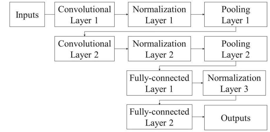
gradient-based optimizer is used to minimize the loss function. Figure 2 illustrates the 235
architecture of the CNN networks used in this study. 236
[Figure 2 is to be inserted about here] 237
The long short term memory networks (LSTM) (Hochreiter et al., 1997) is a special 239
type of recurrent neural networks (RNNs). RNNs contain a feed back connections that 240
allows past information to affect the current output, thus is very effective for tasks 241
involving sequential inputs (Lecun et al., 2015). As an extension of the conventional 242
RNNs, LSTM introduces a special so-called memory cell, which acts like an 243
accumulator, to learn long-term dependency in a sequence, and make the optimization 244
much easier. This cell is self-connected and will copy its own real-valued state and 245
accumulate the external input. Simultaneously each cell is controlled by three 246
multiplicative units –the input, output and forget gates—to determine whether to forget 247
past cell status or to deliver output to the last state, which allow LSTM store and access 248
information over long periods. Following the work of Graves (2013), the formulation 249
are shown as follows: 250
1 1 1 1 1 1 1 tanh tanht xi t hi t ci t i
t xf t hf t cf t f
t t t t xc t hc t c
t xo t ho t co t o
t t t
i W x W h W c b
f W x W h W c b
c f c i W x W h b
o W x W h W c b
h o c
251
Where i, f ,o represent the input, forget and output gate; c is the memory cell; 252
is the logistic sigmoid function; h is a hidden vector; W and b are gate matrix 253
and bias term. 254
CNNs is good at dealing with spatially related data while the LSTM is good at 255
temporal signals. Combination of these two methods can make use of the best of both 256
of the raw input and then feed them to the LSTM networks (hereinafter referred to as 258
ConvLSTM). In this study, predictors from the past 7 days are used to estimate daily 259
rainfall. The structure of the convolutional layers are just the same as previously 260
mentioned. And 400 hidden layers are set up in the LSTM, which is also implemented 261
in tensorflow (Abadi et al., 2016) under python platform. 262
Support Vector Machine 263
The Support Vector Machine (SVM) was first developed by Vapnik (1995) for 264
binary classification. The principle of SVM algorithm is to find the optimal separation 265
hyperplane between two classes by maximizing the boundary margin between the 266
closest points of the class on the boundaries (Sehad, 2017). These points are called 267
support vectors. 268
In SVM regression, the input X is first mapped into a higher dimension feature 269
space, and then a linear model can be constructed as follows (Cover, 1965; Smola, 270
1996): 271
,
j j
j
f X w
w g X b272
Where gj denotes a set of nonlinear transformations, wand b are model 273
parameters to be calibrated. Defining the-insensitive loss function L
y f X w,
,
274
(Vapnik, 1995): 275
0 ,
, ,
,
if y f X w L y f X w
y f X w otherwise
276
1
1
, ,
n
emp i i
i
R w L y f X w n
278
Following Haykin (2003)’s regularization theory, by introducing (non-negative) 279
slack variables i , i* to measure the deviation of training samples outside -280
insensitive zone, the parameters w and b are estimated by minimizing the cost 281 function: 282
* 1 * * 1 min 2 , , . . 0 0 N i i i i i i i i i w C y f X wy f X w s t
283where C is a positive real constant. This optimization problem can be solved by the 284
method of Lagrangian multipliers (Haykin, 2003): 285
*
1(X )
N
i i i
i
w g
286
where iand i* are the Lagrange multipliers, which are positive real constants. 287
In this study, the SVM model is implemented in sklearn (Pedregosa et al., 2011) 288
under python platform. The training of SVM includes selecting the kernel function, and 289
determining the model parameters C and Gamma. These parameters are optimized 290
through the grid search mechanism (Baesens et al., 2002), and C=10, Gamma=0.001 291
and radial basis function are used in this study. 292
Quantile Mapping Method 293
simple approach that has been successfully used in hydrologic studies (e.g., Boé et al., 295
2008). It uses the cumulative frequency curve of the observed precipitation to correct 296
the simulated rainfall so that the corrected rainfall will have the same cumulative 297
frequency curve with the observed one. Figure 3 illustrates how quantile mapping 298
method works. For each grid, calculate the cumulative frequency function of the 299
simulated precipitation ( CFsim( )p ) and the observed precipitation ( CFobs( )p ), 300
respectively. Then for a specific precipitation in the validation period Prevali, we can 301
calculate its frequency on CFsim( )p as CFsim1(Prevali). And then the corresponding 302
precipitation on cumulative frequency function of observed rainfall is just the corrected 303
precipitationPrecorr CFobs(CFsim1(Prevali))
.
304
[Figure 3 is to be inserted about here] 305
3.2 Statistical evaluation based on gauge rainfall data 306
To qualitatively evaluate the downscaling methods, the following metrics were 307
adopted: relative bias (RB), and the root mean square error (RMSE), which were used 308
to show the error and bias of the simulated precipitation compared with observed 309
rainfall data (Ebert et al. 2007; Schaefer 1990); the correlation coefficient (CC), which 310
aims to show the consistency between the predicted rainfall and the observed rainfall. 311
The metrics are calculated as follows: 312
313
1
1
(
)
N
i i
i T
i t
P
G
RB
G
21
1 N
i i
i
RMSE P G
N
315 _ _ 1 _ _ 2 2 1 1 ( )( ) ( ) ( ) N i i i N N i i i iG G P P CC
G G P P
316where Pi and Gi denote the predicted rainfall and observed gauge rainfall, 317
respectively. 318
3.3 Evaluation through hydrological modeling 319
Description of the Distributed Hydrological Model and Model Validation 320
The hydrological model used in this study is a distributed geomorphology-based 321
hydrological model (GBHM) developed by Yang et al. (1998, 2002, 2004). In the 322
GBHM, the study basin is divided into a number of sub-catchments linked by the river 323
network and ordered by the Horton-Strahler scheme. Then, grids within a sub-324
catchment are grouped into several flow intervals according to the flow distance to the 325
outlet. The runoff generated from the grids within a flow interval contributes to the 326
main stream with the same flow distance, and each grid is represented by a number of 327
topographically similar “hillslope-valley” systems, which is the basic unit of the 328
hydrological simulation (Yang et al. 2002, 2015). 329
The GBHM mainly consists of a hillslope module and a kinematic wave flow 330
routing module (Yang et al. 2002, 2004). In the hillslope module, the GBHM simulates 331
the hydrological processes, including interception, evapotranspiration, infiltration, 332
overland flow, unsaturated flow and groundwater flow. Evapotranspiration is calculated 333
in addition to transpiration from the root zone. The topsoil is divided into several layers 335
according to depth, and the vertical soil water movement is described using the 336
Richards equation. Overland flow is described using the one-dimensional kinematic 337
wave equation. Subsurface flow along the hillslope occurs when the soil water content 338
exceeds field capacity. The groundwater aquifer (corresponding to each grid) is 339
discretized and treated as an individual storage compartment. The water exchange 340
between the groundwater and river channel is expected to be steady and is estimated 341
using Darcy’s law (Yang et al. 2002). Most model parameters are defined according to 342
their physical meaning, either based on in situ measurements or regional databases. 343
Only a few parameters must be calibrated, such as the hydraulic conductivity of the 344
groundwater. 345
In this study, 170 sub-catchments are divided with a grid resolution of 2 km, as 346
suggested by Yang et al. (2001) and Miao et al. (2016). The GBHM simulates the 347
hydrological processes at the hourly time step, and is calibrated for the period of 2007-348
2010, and is validated for the period of 2011-2013. The Nash and Sutcliffe coefficient 349
(NSE) and relative bias (RB) are adopted to evaluate the model performance and are 350
where Qobst and Qsimt denote the observed and simulated discharge and Qobs 354
denotes the average values of the observed discharges during the simulation period T. 355
Table 1 contains the calibration and validation results obtained from using gauge 356
rainfall input data for the model. The NSE values for the calibration and validation 357
period are greater than 0.8, and the absolute values of RB are less than 0.05, indicating 358
that GBHM has good performance in the study basin. 359
[Table 1 is to be inserted about here] 360
4. Results and Discussion 361
4.1 Precipitation Estimation Performance With different Predictors 362
In the past studies, many predictors have been used for precipitation downscaling, 363
such as geopotential height (e.g., Kidson and Thompson 1998; Zorita and von Storch 364
1999), sea level pressure (Cavazos 1999), geostrophic vorticity (Wilby et al. 1998), or 365
wind speed (Murphy 1999). The choice of the predictors vary across different regions, 366
characteristics of the large-scale atmospheric circulation, seasonality and 367
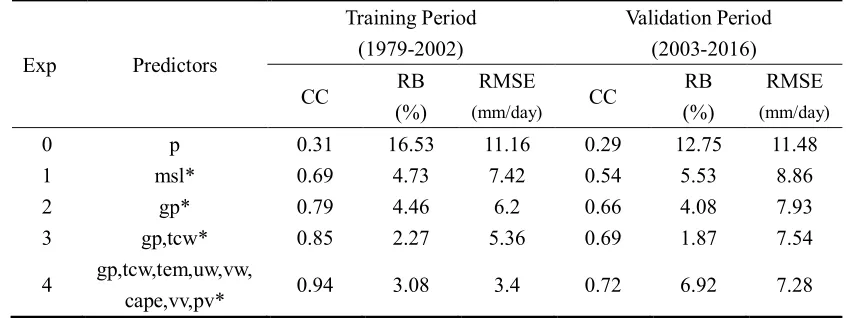
geomorphology (Anandhi et al. 2009). So in this section, we designed four experiments 368
to evaluate the forecast performance of different predictors. As listed in Table 2, 369
Experiment 0 represents the original ECMWF- Interim precipitation; Experiment 1 uses 370
the mean sea level pressure as predictor; Experiment 2 uses the geopotential height at 371
500/700/850/925/1000hpa as predictors; Experiment 3 uses the geopotential height at 372
500/700/850/925/1000hpa as well as the total column water as predictors; Experiment 373
4 uses as much climatology variables as possible as predictors, including all the 374
networks as downscaling method. Models were trained during the period from 1979 to 376
2002, and were validated from 2003 to 2016. 377
Table 2 lists the metrics of results of these experiments (Note that the indexes are 378
calculated for each grid respectively, and the average value for these indexes is shown 379
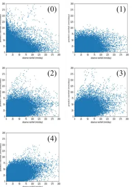
in Table 2; same in Table 3 and Figure 5). Precipitation estimations are plotted against 380
observed ones in Figure 4. Results of experiment 0 shows a relatively low correlation 381
coefficient with observed data (with CC of 0.29) (for validation period, the same 382
hereafter), along with an overestimation of the precipitation (with RB of 12.75%), the 383
root-mean-square error is 11.48mm/day. These metrics indicate a bad performance of 384
original ERA-interim rainfall. Results of experimental 1-4 all outperform original 385
ERA-interim rainfall. Specifically, CC, RB and RMSE values for Experiment 1 is 0.54, 386
5.53%, 8.86 mm/day. All metrics shows an improvement over Experiment 0, but far 387
from enough; and the scatter plots show that it severely underestimates most high-388
intensity rainfall. The CC, RB and RMSE values for Experiment 2 is 0.66, 4.08%, and 389
7.93, and the scatter plot indicates the model could well simulate the high-intensity 390
rainfall. In Experiment 3, CC value further increases to 0.69. Experiment 4 gives the 391
highest CC value of 0.72. 392
[Table 2 is to be inserted about here] 393
[Figure 4 is to be inserted about here] 394
Overall, using as much meteorological variables as possible is conducive to 395
improving the accuracy of downscaling rainfall. Among all meteorological variables, 396
complexity of model, we suggest that the combination of geopotential height and total 398
water vapor might be reasonable. 399
4.2 Precipitation Estimation Performance of different Methods 400
In this section, we compare the performance of different downscaling methods. 401
Quantile mapping method, CNN networks, SVM, and ConvLSTM networks are used 402
as downscaling methods for Experiment 5-8, respectively. Experiment 5 uses ERA-403
interim precipitation as predictor, and Experiment 6-8 use geopotential height at 404
500/700/850/925/1000hpa and total column water as predictors. 405
Metrics and scatter plots are shown in Table 3 and Figure 5, respectively. 406
Experiment 5 use the traditional Quantile mapping method. Its improvement upon 407
original ERA-interim precipitation is very limited. The CC value is only 0.54, and the 408
RMSE value is 10.01mm/day. However, it is worth to mention that only in Experiment 409
5, performance in validation period is comparable to training period, which may be due 410
to its simple model structure and fewer model parameters. While for other complex 411
models, performance in training period evidently exceeds validation period, which 412
reminds us that we should be cautious whether the overfitting phenomena would lead 413
to bad results in operation. Experiment 6 is the same as Experiment 3 in section 4.1, 414
and we will not repeat it here. The SVM is used as training method in Experiment 7, 415
the CC, RB and RMSE values for which are 0.65, -5.05% and 7.91 mm/day. Although 416
its evaluation indexes are comparable to Experiment 6, its scatter plots show that it 417
could barely simulate the high intensity rainfall in the study area (although some study 418
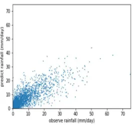
greatly limits its availability in hydrological simulation. Alternatively, if we change to 420
draw the area mean precipitation, as shown in figure 6, the SVM methods can give 421
reasonable results. Performance of Experiment 8 (use ConvLSTM) gives the best 422
evaluation indexes, with CC value of 0.74, RB value of 1.73% and RMSE value of 7.17 423
mm/day. 424
[Table 3 is to be inserted about here] 425
[Figure 5 is to be inserted about here] 426
[Figure 6 is to be inserted about here] 427
Overall, the performance of these downscaling methods gradually increases 428
according to the order of Quantile mapping, SVM, CNN networks, and ConvLSTM 429
networks. 430
4.3 Application of Methods in Precipitation Forecast 431
To further estimate the robustness of the network, in this part we applied the trained 432
network in precipitation forecasting based on the S2S ECMWF hindcast products. For 433
simplicity, only the geopotential height at 500/700/850/925/1000hpa and total water 434
vapor content are used as the predictors in this section (Note that only geopotential is 435
available in S2S ECMWF hindcasts, but it can be transferred to geopotential height by 436
multiply by a constant value of g = 9.80665), and ConvLSTM networks is used as the 437
training model. For the 11 ensemble models, we first obtain the adjusted precipitation 438
using the outputs of each model respectively, and then calculate their average as the 439
final result. 440
adjusted precipitation in the validation period as a function of forecast lead time. We 442
can see that the performance of the corrected precipitation always outperforms the 443
direct output of S2S-ECMWF. For the Day 1 forecast, the correlation coefficient 444
between the corrected precipitation and the observed precipitation is 0.58, slightly 445
lower than the result of experimental 3 in section 4.1 (with CC of 0.69), but significantly 446
better than the S2S-ECMWF precipitation (with CC of 0.36). The difference of the 447
correlation coefficient is 0.22. The CC values decrease sharply with the increase of the 448
lead time. For the Day 15 forecast, the CC value of the corrected precipitation and S2S 449
ECMWF drop to 0.21 and 0.19 respectively, with a difference of only 0.02. In summary, 450
the corrected precipitation is superior to the S2S-ECMWF throughout all the lead time, 451
but the superiority gradually decrease with the increase of the lead time. 452
[Figure 7 is to be inserted about here] 453
For the original ECMWF precipitation prediction, the uncertainty mainly comes 454
from two sources. The first is dynamical deviation from the true atmosphere evolution, 455
and the second is parameterization error due to imperfect description of unresolved 456
scale physical processes. Compare to the original ECMWF precipitation prediction, the 457
downscaled precipitation can eliminate the parameterization error to some extent: for 458
the one hand, it uses the observed precipitation, but the GCM is not calibrated locally; 459
for the other hand, the straightforward ConvLSTM network uses a top-down 460
parameterization paradigm, and might be more efficient when properly calibrated. 461
When the lead time is short, both of two kinds of uncertainty sources cannot be ignored, 462
advantage over S2S-ECMWF precipitation prediction. As forecast lead time extends, 464
the first kind of error (dynamical deviation) gradually dominates due to the chaotic 465
effect, and the superiority of the ConvLSTM downscaling method gradually disappears. 466
4.4 Application in Hydrological Simulation 467
After calibration and validation, the GBHM is run using the observed rainfall, the 468
original ERA-interim rainfall and the downscaled rainfall (using geopotential height at 469
500/700/850/925/1000hpa and total column water as predictors, ConvLSTM networks 470
as downscale method, i.e., Experiment 8 in 4.2) as input data, respectively. All 471
simulations use the hydrological state at the end of 2010 as initial condition, which is 472
obtained from continuous running GBHM using gauge rainfall as input. 473
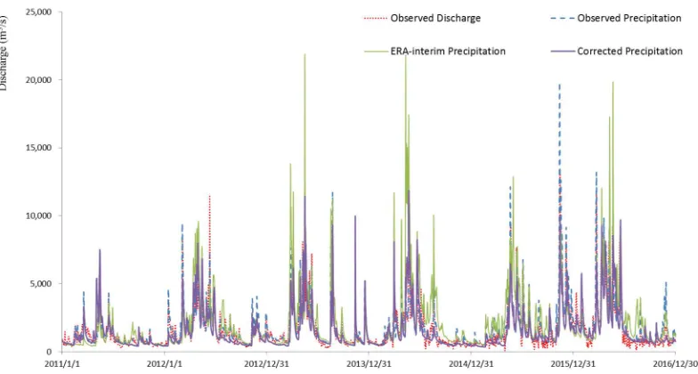
Table 4 gives the evaluation indexes and figures 8 compares the streamflow 474
simulation results using three sets of rainfall input at Hengshan station from 2011 to 475
2016, respectively. The simulation using observed rainfall data agrees well with the 476
observed discharge, with NSE value of 0.82 and RB value of 7%. However, the original 477
ERA-interim rainfall forced simulation is almost completely useless, with a NSE value 478
of 0.06. It severely overestimates most flood peaks as shown in figure 8, and 479
overestimate 24% of the total runoff. The simulation using the adjusted rainfall provides 480
reasonable result, with NSE value of 0.64 and RB value of -10%. It is close to the 481
observed rainfall forced simulation, and far better than the original ERA-interim rainfall 482
forced simulation. Hydrological systems are non-linear systems, uncertainties in 483
precipitation inputs may be magnified when it is transferred to runoff, which makes the 484
[Table 4 is to be inserted about here] 486
[Figure 8 is to be inserted about here] 487
5. Summary and conclusions 488
In this study, we proposed a new method for precipitation downscaling by 489
combining CNN and LSTM, based on model resolved circulation dynamics. This 490
method was tested for precipitation estimation or prediction in Xiangjiang River Basin 491
in south China, which located in the East Asian monsoon region. The results show that 492
this method has advantages over the traditional quantile mapping method or SVM based 493
method. The downscaled rainfall was further evaluated through a distributed 494
hydrological model. The major conclusions can be summarized as follows: 495
(1) 4 Experiments using different circulation predictors are designed to test the 496
effectiveness of those predictors. Results show that using as much 497
meteorological variables as possible is conducive to improving the rainfall 498
estimation. While using mean sea level alone can only provide limited 499
improvement. Among all meteorological variables, the geopotential height 500
might be the most important one. Considering both accuracy and complexity 501
of model, we suggest that the combination of geopotential height and total 502
water vapor might be reasonable. 503
(2) Another 4 Experiments are designed to compare the different performance of 504
Quantile Mapping method, SVM, CNN networks, and ConvLSTM networks. 505
Precipitation estimated by ConvLSTM networks give the best performance 506
Quantile Mapping method, with correlation coefficient of 0.69, 0.65, 0.54 508
respectively. We also found that method based on SVM could not predict those 509
very high intensity rainfall. 510
(3) The trained ConvLSTM networks are applied to S2S-ECMWF hindcast 511
datasets to further test its robustness. We find the corrected precipitation is 512
superior to the original S2S-ECMWF precipitation all the time, but the 513
superiority gradually decreased with the increase of the lead time. We think the 514
improvement mainly comes from the use of observed data and the effective 515
networks, which can reduce the parameterization error. But when the lead time 516
extends, the parameterization error becomes subordinate. Thus the superiority 517
of proposed method gradually fades away. 518
(4) Different rainfall inputs are fed into the distributed hydrological model. The 519
original EAR-Interim rainfall shows little usage in hydrological simulation 520
with a NSE of 0.06 and RB of 24%. While the corrected rainfall forced 521
simulation improves the NSE to 0.64 and reduce RB to -10%, which is 522
comparable to the simulation forced by observed rainfall. This further proves 523
the value of the proposed method. 524
525
References 526
Abadi M, Agarwal A, Barham P, et al. TensorFlow: Large-Scale Machine Learning on
527
Heterogeneous Distributed Systems[J]. 2016.
Anandhi A, Srinivas VV, Nanjundiah RS, Nagesh Kumar D (2008) Downscaling precipitation to
529
river basin in India for IPCC SRES scenarios using support vector machine. Int J Climatol
530
28:401–420.
531
Anandhi A , Srinivas V V , Kumar D N , et al. Role of predictors in downscaling surface temperature
532
to river basin in India for IPCC SRES scenarios using support vector machine[J].
533
International Journal of Climatology, 2009, 29(4):583-603.
534
Baesens B , Viaene S , Gestel T V , et al. An empirical assessment of kernel type performance for
535
least squares support vector machine classifiers[C]. International Conference on
536
Knowledge-based Intelligent Engineering Systems & Allied Technologies. IEEE, 2002.
537
Bauer P, Thorpe A , Brunet G . The quiet revolution of numerical weather prediction [J]. Nature,
538
2015, 525(7567):47-55.
539
Benestad R. Novel methods for inferring future changes in extreme rainfall over Northern
540
Europe[J]. Climate Research, 2007, 34(3):195-210.
541
Benestad R. and J. Haugen, 2007: On complex extremes: Flood hazards and combined high
spring-542
time precipitation and temperature in Norway. Climatic Change, 85, 381–406,
543
doi:10.1007/s10584-007-9263-2.
544
Boé J., Terray L., Habets F., Martin E.. Statistical and dynamical downscaling of the Seine basin
545
climate for hydro-meteorological studies. International Journal of climatology, 2007, 27:
546
1643-1655.
547
Cavazos, T., 1999: Large-scale circulation anomalies conducive to extreme precipitation events and
548
derivation of daily rainfall in northeastern Mexico and southeastern Texas. J. Climate, 12,
549
1506–1523.
Christensen J H, Machenhauer B, Jones R G, et al. Validation of present-day regional climate
551
simulations over Europe: LAM simulations with observed boundary conditions[J]. Clim
552
Dyn, 1997, 13(7):489-506.
553
Cover, T.M., 1965. Geometrical and statistical properties of systems of linear inequalities with
554
applications in pattern recognition. IEEE Transactions on Electronic Computers EC-14,
555
326–334.
556
Dai, Y., W. Shangguan, Q. Duan, B. Liu, S. Fu, and G. Niu, 2013: Development of a China dataset
557
of Soil hydraulic parameters using Pedotransfer functions for Land surface modeling. J. 558
Hydrometeor, 14, 869–887. doi:10.1175/JHM-D-12-0149.1.
559
Dee D P, Uppala S M, Simmons A J, et al. The ERA‐Interim reanalysis: configuration and
560
performance of the data assimilation system[J]. Quarterly Journal of the Royal
561
Meteorological Society, 2011, 137(656):553-597.
562
Graves A . Generating Sequences With Recurrent Neural Networks[J]. Computer Science, 2013.
563
Ghosh S. SVM-PGSL coupled approach for statistical downscaling to predict rainfall from GCM
564
output[J]. Journal of Geophysical Research Atmospheres, 2010, 115(D22).
565
Guhathakurta P. Long lead monsoon rainfall prediction for meteorological sub-divisions of India
566
using deterministic artificial neural network model[J]. Meteorology & Atmospheric
567
Physics, 2008, 101(1-2):93-108.
568
Hanssen‐Bauer, I., C. Achberger, R. Benestad, D. Chen, and E. Forland (2005), Statistical
569
downscaling of climate scenarios over Scandinavia, Clim. Res., 29(3), 255–268.
570
Haykin, S., 2003. Neural Networks: A comprehensive foundation. Fourth Indian Reprint, Pearson
571
Education, Singapore, pp. 842.
Hochreiter S, Schmidhuber J. Long Short-Term Memory[J]. Neural Computation, 1997,
9(8):1735-573
1780.
574
Hope, P. K. (2006), Projected future changes in synoptic systems influencing southwest western
575
australia, Climate Dynamics, 26(7-8), 765–780.
576
Ioffe, S., and C. Szegedy (2015), Batch normalization: Accelerating deep network training by
577
reducing internal covariate shift, in International conference on machine learning, pp. 448–
578
456.
579
James W Taylor. A quantile regression neural network approach to estimating the conditional
580
density of multi-period returns. Journal of Forecasting, 19(4):299–311, 2000.
581
Kidson, J. W., and C. S. Thompson, 1998: A comparison of statistical and model-based downscaling
582
techniques for estimating local climate variations. J. Climate, 11, 735–753.
583
Kang, I. S., and Coauthors, 2002: Intercomparison of the climatological variations of Asian summer
584
monsoon precipitation simulated by 10 GCMs. Climate Dyn., 19, 383–395.
585
Kannan, S., and S. Ghosh (2013), A nonparametric kernel regression model for downscaling
586
multisite daily precipitation in the mahanadi basin, Water Resources Research, 49(3),
587
1360–1385.
588
Lecun Y , Bengio Y , Hinton G . Deep learning.[J]. Nature, 2015, 521(7553):436.
589
Li, Y., and I. Smith (2009), A statistical downscaling model for southern australia winter rainfall,
590
Journal of Climate, 22(5), 1142–1158.
591
Li, Z., D.W. Yang, B. Gao, Y. Jiao, Y. Hong, and T. Xu, 2015: Multiscale hydrologic applications
592
of the latest satellite precipitation products in the Yangtze River basin using a distributed
hydrologic model. J. Hydrometeor., 16, 407-426, doi: http://dx.doi.org/10.1175/JHM-D-594
14-0105.1..
595
Meehl, G. A., et al., Climate Change 2007: The Physical Science Basis. Contribution of Working
596
Group I to the Fourth Assessment Report of the Intergovernmental Panel on Climate
597
Change, chap. Global Climate Projections, Cambridge University Press, Cambridge,
598
United Kingdom and New York, NY, USA, 2007.
599
Miao Q , Yang D , Yang H , et al. Establishing a rainfall threshold for flash flood warnings in China’
600
s mountainous areas based on a distributed hydrological model[J]. Journal of Hydrology,
601
2016, 541(541):371-386.
602
Murphy, J., 1999: An evaluation of statistical and dynamical techniques for downscaling local
603
climate. J. Climate, 12, 2256–2284.
604
Murphy, J., et al. (2000), Predictions of climate change over Europe using statistical and dynamical
605
downscaling techniques, International Journal of Climatology, 20(5), 489–501.
606
Nijssen, B. and D.P. Lettenmaier, 2004: Effect of precipitation sampling error on simulated
607
hydrological fluxes and states: anticipating the global precipitation measurement satellites.
608
J. Geophys. Res., 109, D02103. doi:10.1029/2003JD003497.
609
Norton C W, Chu P S, Schroeder T A. Projecting changes in future heavy rainfall events for Oahu,
610
Hawaii: A statistical downscaling approach[J]. Journal of Geophysical Research
611
Atmospheres, 2011, 116(D17):-.
612
Pan, B., and Z. Cong (2016), Information analysis of catchment hydrologic patterns across temporal
613
scales, Advances in Meteorology, 2016.
Pan, Baoxiang & Hsu, Kuolin & AghaKouchak, Amir & Sorooshian, Soroosh. (2019). Improving
615
Precipitation Estimation Using Convolutional Neural Network. Water Resources Research.
616
10.1029/2018WR024090.
617
Panofsky, H. A., and G. W. Brier (1968), Some Application of Statistics to Meteorology, 224 pp.,
618
Pa. State Univ., University Park, Pa
619
Penman, H. L., 1948: Natural evaporation from open water, bare soil and grass. Proc. of the Roy.
620
Soc. Lond. Ser. A. Math. Phys. Sci., 193, 1doi:10.1098/rspa.1948.0037.
621
Prudhomme, C., N. Reynard, and S. Crooks (2002), Downscaling of global climate models for flood
622
frequency analysis: Where are we now?, Hydrol. Processes, 16(6), 1137–1150,
623
doi:10.1002/hyp.1054.
624
Schoof, J. T., and S. Pryor (2001), Downscaling temperature and precipitation: A comparison of
625
regression-based methods and artificial neural networks, International Journal of
626
climatology, 21(7), 773–790.
627
Scikit-learn: Machine Learning in Python, Pedregosa et al., JMLR 12, pp. 2825-2830, 2011.
628
Sehad M, Lazri M, Ameur S. Novel SVM-based technique to improve rainfall estimation over the
629
Mediterranean region (north of Algeria) using the multispectral MSG SEVIRI imagery[J].
630
Advances in Space Research, 2016, 59(5):1381-1394.
631
Shen Y, Xiong A, 2016: Validation and comparison of a new gauge-based precipitation analysis
632
over mainland China. Int. J. Climatol., 36, 252-265. doi: 10.1002/joc.4341.
633
Shi X, Chen Z, Hao W, et al. Convolutional LSTM Network: a machine learning approach for
634
precipitation nowcasting[C]// International Conference on Neural Information Processing
635
Systems. 2015.
Smola, A. J. (1996), Regression Estimation with Support Vector Learning Machines, Technische
637
Universitat Munchen, Munich, Germany.
638
Stephens G L , L'Ecuyer T , Forbes R , et al. Dreary state of precipitation in global models[J].
639
Journal of Geophysical Research Atmospheres, 2010, 115(D24):-.
640
Tapiador F J , Roca, Rémy, Genio A D , et al. Is precipitation a good metric for model performance?
641
[J]. Bulletin of the American Meteorological Society, 2018.
642
Tripathi, S., V. Srinivas, and R. S. Nanjundiah (2006), Downscaling of precipitation for climate
643
change scenarios: a support vector machine approach, Journal of hydrology, 330(3- 4),
644
621–640.
645
Vandal, T., E. Kodra, S. Ganguly, A. Michaelis, R. Nemani, and A. R. Ganguly (2017), Deepsd:
646
Generating high resolution climate change projections through single image
super-647
resolution, in Proceedings of the 23rd ACM SIGKDD International Conference on
648
Knowledge Discovery and Data Mining, pp. 1663–1672, ACM.
649
Vapnik, V.N., 1995. The Nature of Statistical Learning Theory. Springer Verlag, New York.
650
Vitart, F. (2004), Monthly forecasting at ecmwf, Monthly Weather Review, 132(12), 2761–2779.
651
Vitart, F., C. Ardilouze, A. Bonet, A. Brookshaw, M. Chen, C. Codorean, M. Déqué, L. Ferranti, E.
652
Fucile, M. Fuentes, et al. (2017), The subseasonal to seasonal (s2s) prediction project
653
database, Bulletin of the American Meteorological Society, 98(1), 163–173.
654
Wang, B., I. S. Kang, and J. Y. Lee, 2004: Ensemble simulation of Asian–Australian monsoon
655
variability by 11 AGCMs. J. Climate, 17, 803–818.
656
Wilby, R. L., and T. M. L. Wigley, 2000: Precipitation predictors for downscaling: Observed and
657
general circulation model relationships. Int. J. Climatol., 20, 641–661.
Yang, D W, T Koike, and H Tanizawa, 2004: Application of a distributed hydrological model and
659
weather radar observations for flood management in the upper Tone River of Japan.
660
Hydrological Processes, 18, 3119-3132. doi:10.1002/hyp.5752.
661
Yang, D, S Herath, and K Musiake, 2001: Spatial resolution sensitivity of catchment
662
geomorphologic properties and the effect on hydrological simulation. Hydrol. Process., 15,
663
2085-2099. doi:10.1002/hyp.280.
664
Yang, D., S. Herath, and K. Musiake, 2002: A Hillslope-based hydrological model using catchment
665
area and width functions. Hydrol. Sci. J., 47, 49-65. doi:10.1080/02626660209492907.
666
Yang, D.W., B. Gao, Y. Jiao, H.M. Lei, Y.L. Zhang, H.B. Yang, and Z.T. Cong, 2015: A distributed
667
scheme developed for eco-hydrological modeling in the upper Heihe river. Sci. China Earth 668
Sci., 58, 36–45. doi:10.1007/s11430-014-5029-7.
669
Yang, D.W., S. Herath, and K Musiake, 1998: Development of a geomorphology-based
670
hydrological model for large catchments. Proc. Hydraul. Eng., 42, 169–174.
671
doi:10.2208/prohe.42.169.
672
674
Figure 1. Study basin and locations of the hydrological station and meteorological stations
675 676 677
678
Figure 2. Architecture of the CNN networks used in this study
683 684
685
Figure 3 Illustration of the quantile mapping method
686 687
688
Figure 4 Scatterplots of estimated precipitation using different predictors against observed
689
precipitation (daily scales): (0) Original ERA-Interim precipitation, (1) Sea level mean pressure,
(2) Geopotential Height, (3) Geopotential Height filed and total column water, and (4) all
691
circulation variables described in section 2.2
692
693
Figure 5 Scatterplots of estimated precipitation using different downscaling methods against
694
observed precipitation (daily scales): (5) Quantile mapping, (6) CNN networks, (7) SVM, and
695
(8) ConvLSTM networks
696 697 698 699
700
Figure 6 Similar to figure 5 (7), but for area mean precipitation
704
Figure 7 Predictive skill of S2S ECMWF precipitation and the corrected precipitation in the
705
validation period as function of forecast lead time
706 707 708
709
Figure 8 Comparison of the hydrographs at Hengshan station among the observation (reference),
710
observed precipitation-driven simulation, ERA-interim precipitation -driven simulation and
711
corrected precipitation-driven simulation
Table 1. GBHM performance of daily discharge simulation during the calibration and validation
716
periods at Hengshan Station
717
Period NSE RB
Calibration period 0.89 0.04 Validation period 0.88 0.02
Table 2. Performance of downscaled precipitation using different predictors
718
Exp Predictors
Training Period (1979-2002)
Validation Period (2003-2016)
CC RB (%)
RMSE
(mm/day) CC
RB (%)
RMSE
(mm/day)
0 p 0.31 16.53 11.16 0.29 12.75 11.48 1 msl* 0.69 4.73 7.42 0.54 5.53 8.86 2 gp* 0.79 4.46 6.2 0.66 4.08 7.93 3 gp,tcw* 0.85 2.27 5.36 0.69 1.87 7.54
4 gp,tcw,tem,uw,vw,
cape,vv,pv* 0.94 3.08 3.4 0.72 6.92 7.28 Note: p represents original ERA-interim precipitation; msl represents mean sea level pressure; gp
719
represents geopotential height; tcw represents total column water; tem represents air temperature;
720
cape represents convective available potential energy; uw represents u wind component; vw
721
represents v wind component; vv represents vertical velocity; pv represents potential vorticity.
722
Table 3. Performance of downscaled precipitation using different downscaling methods
723
Exp Method
Training Period (1979-2002)
Validation Period (2003-2016)
CC RB (%)
RMSE
(mm/day) CC
RB (%)
RMSE
(mm/day)
0 ERA-interim 0.31 16.53 11.16 0.29 12.75 11.48 5 QM 0.54 0.21 9.77 0.54 -2.82 10.01 6 CNN 0.85 2.27 5.36 0.69 1.87 7.54 7 SVM 0.70 2.31 7.33 0.65 -5.05 7.91 8 ConvLSTM 0.85 2.27 5.36 0.73 1.73 7.17
Table 4. Performance of simulations with different precipitation forcing
724
Precipitation Inputs NSE RB(%) Observed Precipitation 0.82 7 Original ERA-interim Precipitation 0.06 24
Corrected Precipitation 0.64 -10