Optimal leverage, its benefits, and the business cycle

econ

stor

www.econstor.eu

Der Open-Access-Publikationsserver der ZBW – Leibniz-Informationszentrum Wirtschaft The Open Access Publication Server of the ZBW – Leibniz Information Centre for Economics

Nutzungsbedingungen:

Die ZBW räumt Ihnen als Nutzerin/Nutzer das unentgeltliche, räumlich unbeschränkte und zeitlich auf die Dauer des Schutzrechts beschränkte einfache Recht ein, das ausgewählte Werk im Rahmen der unter

→ http://www.econstor.eu/dspace/Nutzungsbedingungen nachzulesenden vollständigen Nutzungsbedingungen zu vervielfältigen, mit denen die Nutzerin/der Nutzer sich durch die erste Nutzung einverstanden erklärt.

Terms of use:

The ZBW grants you, the user, the non-exclusive right to use the selected work free of charge, territorially unrestricted and within the time limit of the term of the property rights according to the terms specified at

→ http://www.econstor.eu/dspace/Nutzungsbedingungen By the first use of the selected work the user agrees and declares to comply with these terms of use.

zbw

Working Paper

Optimal leverage, its benefits, and the

business cycle

CFR working paper, No. 11-12

Provided in cooperation with:

Universität zu Köln

Suggested citation: Hess, Dieter; Immenkötter, Philipp (2011) : Optimal leverage, its benefits, and the business cycle, CFR working paper, No. 11-12, http://hdl.handle.net/10419/50004

CFR

CFR

CFR

CFR Working Paper NO. 11

Working Paper NO. 11

Working Paper NO. 11

Working Paper NO. 11-

-

-

-12

12

12

12

Optimal Leverage, its Benefits, and

Optimal Leverage, its Benefits, and

Optimal Leverage, its Benefits, and

Optimal Leverage, its Benefits, and

the Business Cycle

the Business Cycle

the Business Cycle

the Business Cycle

D

D

D

Optimal Leverage, its Benefits,

and the Business Cycle

∗

Dieter Hess

, Philipp Immenk¨

otter

Abstract

We study the effect of the business cycle on optimal capital structure choice and the benefit to leverage. We propose a regime switching model with a state-dependent cash flow process to capture macroeconomic risk in a firm’s cash flow. Our model is parsimonious but still realistic and allows for a wide range of analysis. We find pro-cyclical optimal leverage ratios, benefits to leverage, and costs of operating at a non-optimal leverage. If macroeconomic risk decreases, i.e. earnings become more stable and growth rates less volatile, optimal leverage and its benefits increase due to lower default risk. The regime switching property of EBIT traces observed EBIT paths closely and is applicable to a wide range of corporate valuation models. Our model offers novel empirically testable implications, such as higher tax benefits after the change in macroeconomic risk since the late 1980s and common capital structure adjustments in recessions and around turning points.

Keywords: capital structure; macroeconomic risk; regime switching; benefit to leverage JEL classification: E44; G12; G32

∗_{We are grateful for valuable discussions and comments from Christian Hellwig, Alexander Ludwig, Anna}

Reifenh¨auser, Martin Ruckes, Marliese Uhrig-Homburg, the participants of the research seminars in Cologne and Karlsruhe (KIT), the 14th meeting of the Swiss Society for Financial Market Research (SGF), and the 47th annual meeting of the Eastern Finance Association (EFA).

†_{University of Cologne, Corporate Finance Seminar and CFR Cologne}

‡_{Corresponding author, University of Cologne, Corporate Finance Seminar, contact information:}

1

Introduction

The business cycle is essential for understanding corporate financing decisions. To analyze how the macroeconomic risk affects optimal leverage ratios, we propose a structural model of optimal capital structure that incorporates changing macroeconomic conditions through the firm’s cash flow channel. Our model is parsimonious but at the same time realistic and allows for a wide range of analysis. We show that optimal leverage and its benefits vary pro-cyclically, and a reduction of macroeconomic risk lowers optimal leverage ratios but influences benefits to leverage only marginally. The costs that a corporation faces if it operates at a non-optimal leverage are higher in recessions.

In contrast to previous approaches, we model earnings before interest and taxes (EBIT) with a stochastic process that depends on the business cycle. In expansions EBIT follow a positive trend while in contractions they decrease on average. The turning points of the economy are determined stochastically by a Markov chain. Following Goldstein, Ju, and Le-land (2001) and the trade-off theory, the firm chooses its optimal financing mix by balancing tax benefits and default costs which in turn depend on the macroeconomic conditions. As a result we find that optimal capital structures and benefits to leverage strongly differ in expansions and recessions.

Our model shows that optimal leverage choice varies pro-cyclically with the business cycle. In expansions firms choose a higher amount of debt for financing their investments, while they turn to equity financing in contractions. Positive growth expectations decrease a firm’s default risk and increase its debt capacity. In contrast, default is more likely in recessions and the firm behaves optimal by choosing a higher amount of equity to reduce default risk.

The benefit to leverage, defined as the ratio of the levered and unlevered firm value, is pro-cyclical as well. Estimating the parameters of our model to reflect S&P500 firms, we find that by issuing debt the unlevered asset value of the firm is increased by 5% in expansions and by 4% in contractions. Despite increasing default risk, tax shields are important means

to maximize shareholders wealth in contractions. In expansions the levered firm value is 23% higher than in recessions, but the benefits increase only by 1%. Hence, benefits account for only a small fraction of the gain in the levered firm value.

If managers want to determine their firm’s optimal leverage ratios, they need to precisely assess the present state of the economy and the expected growth rate of EBIT. If they fail to identify the present conditions, they come to a non-optimal leverage choice. Firms operating at a non-optimal leverage ratio face costs of being over- or underlevered. We find that these costs are higher in recessions than in expansions. In recessions marginal default costs increase more rapidly with outstanding debt which makes being overlevered more costly in this state. If managers issue too little debt in a contraction, then they miss a substantial amount of tax benefits which are an important way to create shareholder value since earnings will decline on average. For a small deviation from the optimum, the costs are only a small fraction of the levered firm value, but if the optimum changes due to a switch of the state, then the firm faces high costs. If capital structure adjustments are costly, then the firm adjusts their leverage more often at turning points of the economy, because there it is more likely that the increase in value exceeds the adjustment costs. Besides this finding, leverage adjustments should generally be more common in recessions because the costs of being over-or underlevered are higher in this state.

As observed by Stock and Watson (2002), macroeconomic risk has changed over time. After the 1980s, recessions became milder and economic growth less volatile. This shift in macroeconomic conditions affects corporate financing policies. Our model shows that mild recessions and less volatile growth rates lead to higher levered firm values, because the loss of cash flows in recessions is smaller. As a response optimal leverage increases due to a reduction in default risk. However, the benefits to leverage are hardly affected by the changing conditions. The fraction of the levered firm value that corresponds to the benefits to leverage varies only slightly. If firms behave optimal they can keep the benefits to leverage at the same level, independent of the state of the economy.

Our theoretical results on pro-cyclical leverage ratios explain recent empirical findings by Korteweg (2010) who assesses a significant positive difference in optimal leverage ratios over the business cycle. Our findings are also in line with Covas and Den Haan (2010) who come to the result of pro-cyclical debt issuances. In their empirical study, Korajczyk and Levy (2003) analyze observed leverage ratios on the basis of financial constraints and state that financially unconstrained firms have countercyclical leverage ratios. Our model addresses optimal rather than observed leverage ratios, which are not necessarily identical. For example, according to the trade-off theory a profitable firm operates at a high optimal leverage ratio. But over time high retained earnings decrease the observed leverage constantly, so that observed and optimal ratios do not correspond to each other. In our model optimal leverage is not affected by the historic outcomes, it reflects the optimal leverage choice at a certain point in time.

The main distinction of our model to previous approaches is that the firm faces unlimited downward risk once a recession sets in. In constrast, modeling EBIT with a geometric Browian motion multiplied with a state variable that switches between two values to reflect macroeconomic risk (e.g. Hackbarth, Miao, and Morellec (2006)) implies that the economic outlook at the beginning of a recession is rather bright. Once the firm has survived the jump down to a much lower EBIT level at the start of a recession, the upside potential from jumping back to the old level is huge. This leads to the counterintuitive implication that the economic outlook at the beginning of a recession is even brighter than in the middle of an expansion. Hence, the assumption that drift rates rather than the level of EBIT switch is the central distinction in our model. It is mainly responsible for the fact that we find pro-cyclical rather than counter-cyclical leverages to be optimal.

Two independent, recent papers construct a similar framework but have a different fo-cus. Chen (2010) uses regime switching processes to model a firm’s cash flow, the outcome of the economy, and the consumer price index. His analysis focuses on credit spreads and default rates Bhamra, Kuehn, and Strebulaev (2009) combine a structural model with a consumption-based asset pricing model to explain leverage ratios at aggregated and

indi-vidual levels. Their approach integrates the effect of the business cycle in the aggregate consumption and through an additional systematic volatility component. In our analysis we examine the optimal leverage choice, the benefit to leverage, costs of being over- or un-derlevered and changing macroeconomic conditions. Our approach focuses on the effect of state dependent EBIT, not of the consumption in the economy. Moreover, our approach is more parsimonious and we are able to trace the observed effects closely back to our state dependent earnings process.

The rest of the paper is organized as follows: In section 2 we define the economy of the model and in section 3 we use the contingent claims valuation technique to derive analytical functions for the levered firm and debt value. In section 4 we estimate the model’s param-eters and analyze implications on optimal leverage, the benefit to leverage, and changing macroeconomic conditions. Finally, section 5 concludes. Derivations are contained in the appendix.

2

The model

We consider a continuous time economy with a representative firm and two possible states of the economy, i.e., expansion (i = 1) or recession (i = 2). All agents know the present state i0 at all times and its characteristics. The transition from one state to the other is given by a Markov chain Mt with Poisson transition probabilities. The rate of leaving the present state iin the infinitesimal time interval dt is denoted λi. All agents are risk neutral and discount cash flows with the constant risk free rate r. Corporate earnings are taxed at the constant tax rate τ and management acts in best interest of shareholders.

Upon this economy, we consider an infinitely-lived firm whose assets generate stochastic EBIT xt. Because of different earning perspectives in different states of the economy, xt follows a geometric Brownian motion that changes its drift and volatility components at

turning points of the economy, called regime-switching-process:1

dxt =µixt dt+σixt dWt, where i= 1,2 µ1, µ2 ∈R, σ1, σ2 >0, x0 >0

(1)

Uncertainty is modeled through the complete probability space (Ω,F,P), where the σ -algebra F is generated by the Markov chain Mt and standard Brownian motion (Wt)t≥0. The probability measure P is the product of the distribution of dWt and Mt. To obtain a realistic setting of EBIT across the business cycle, we assume µ1 > 0 and µ2 < 0, i.e. the expected earnings growth is positive in an expansion and negative in a recession. The risk of deviation from the present EBIT-trendµi is reflected through the state dependent volatility component σi. The present value of expected perpetually generated after-tax EBIT is the value of the firm’s unlevered assets u(x).

Since the firm’s EBIT is subject to taxation at the constant tax rate τ, the firm has incentives to issue debt in order to generate tax benefits and to create a levered firm value

v(x) exceeding the unlevered asset value u(x). We consider a stationary debt environment according to Leland (1998) where a firm initially issues a certain amount of debt with princi-pal P, fair couponC. Throughout time a constant fraction mof outstanding debt is retired continuously and replaced by the same amount of debt with the same coupon and retirement rate, so that the outstanding amount of debtP is constant over time. Debt is issued at par so that the principal P equals the initial market value of debt d(x0) and the firm has to pay the fair coupon that incorporates the risk of the volatile EBIT process. The value of shareholders equitye(x) is the residual claim to the levered firm valuev(x) after subtraction of the market value of debt d(x).

The issuance of debt bears default risk. We incorporate an endogenous default decision according to Leland and Toft (1996), where the decision to default belongs to the shareholders and default is triggered if EBITxt falls beneath state dependent default thresholds,K1 and

K2. The thresholds correspond to the point where shareholders optimally stop injecting funds into the firm because the cost of remaining active equals its benefits. Since the benefits are state dependent and higher in an expansion due to the positive difference in the growth rates

µ1−µ2, we find thatK1 < K2. In words, the firm will default earlier in a recession than in an expansion. When default occurs, bondholders receive the unlevered asset value less default costs and equity becomes worthless. Default costs are reflected through a state dependent recovery rate 0< αi ≤1, so that the payment to bondholders in case of default corresponds tod(x) = αiu(x),i denoting the present state at time of default.

All claims, such as the levered firm value v(x), the unlevered asset valueu(x), debt value

d(x), and equity value e(x) are state dependent functions of EBIT xt, which is denoted by the index i: v(xt) =        v1(xt) if it= 1 v2(xt) if it= 2 (2)

Initially managers choose the outstanding amount of debt P to maximize the levered firm valuev(x) = vi0(x) and hence the shareholders wealth. The maximum is achieved when the marginal tax benefits equal the default cost. Since the value of the levered firmv(x) depends on the present state, the maximization problem has two solution, namely for each possible present state one solution:

max

P vi(x) i= 1,2 (3)

We define leverage as the ratio of debt and the levered firm value li = di(x)/vi(x). l1 is the leverage in an expansion, l2 in a recession, and l∗i is the optimal ratio that maximizes the levered firm value in the corresponding state i. The benefit to leverage is defined as

bi = vi(x)

−ui(x)

ui(x) and refers to the present value of the expected future benefits of issuing debt

benefits, the maximization of the levered firm value is equivalent to the maximization of the benefits.

3

Valuation of corporate securities

In this section we construct a static contingent claims valuation model with the basic characteristics of Hackbarth, Miao, and Morellec (2006) to derive closed form solutions for the value of the firm’s unlevered asset value, the levered firm value, its outstanding amount of debt, and the value of shareholder’s equity. All claims are denoted as functions of EBIT

xt and dependent on the state i= 1,2.

If the default threshold in expansions K1 is lower than in recessions K2, we have three disjoint regions that can be analyzed separately. We define the region x≤K1 as the default region. Here, the firm is liquidated in both states. Second, K1 < x ≤ K2, defines the transient region where the firm is active in state one, but liquidated in state two. Third, the action region K2 < x, where the firm is active in both states. As shown in section 4, the case of K1 < K2 is sufficient and hence we will not discuss other scenarios.

3.1

Unlevered asset value

Following Mello and Parsons (1992) the value of unlevered assetsu(x) corresponds to the present value of a perpetual claim to after-tax EBIT.

u(x) =_E Z ∞ t e−r(s−t)(1−τ)xs ds x0 =x, i0 =i , i= 1,2 (4)

It can be compared to the value of the firm that does not issue debt. An application of Itˆo’s Lemma to each state of the economy yields a set of ordinary differential equations for the

value of unlevered assetsui:2 1 2x 2_σ2 1u 00 1+µ1xu01 −ru1+λ1(u2−u1) + (1−τ)x= 0 (5) 1 2x 2_σ2 2u 00 2+µ2xu02 −ru2+λ1(u1−u2) + (1−τ)x= 0 (6)

The equation consists of three parts: first, a linear Black-Scholes operator 1₂x2_σ2 iu

00

i+µixu0i− rui captures the change of the unlevered firm value due to the movement of the Brownian motion. The second part λi(uj −ui) is the change in values arising from a regime shift multiplied by the rate of leaving state i. The third part (1−τ)x represents the perpetual claim to after-tax EBIT.

Under the boundary conditions

lim

x→0ui(x)<∞ and limx→∞

ui(x)

x <∞, (7)

the solution to (5) and (6) is

u1(x) =w1·x and u2(x) = w2·x . (8)

with the constants w1 and w2 given by

w1 =− (1−τ)(µ2−r−λ1−λ2) (µ1 −r−λ1)(µ2−r−λ2)−λ1λ2 , (9) w2 =− (1−τ)(µ1−r−λ1−λ2) (µ1 −r−λ1)(µ2−r−λ2)−λ1λ2 . (10)

The unlevered asset value is a linear function of the present level of EBIT. The constant coefficients wi incorporate the growth rate in the present state µi and the possible switch to the other state with a different growth rate. Intuitively, for the considered scenario with

µ1 > µ2, we find thatu1(x)> u2(x). Moreover, the unlevered asset value is independent of

the volatilityσi of EBIT because it is the expected value of the process, reflecting the future drift not the volatility.

3.2

Value of corporate debt

The state dependent value of all outstanding corporate debt di (i = 1,2) is the present value of the continuous coupon payment C and retirement of the principal mP as long as the firm is solvent. Upon default bondholders receive the state dependent unlevered asset value diminished by the recovery rateαi. In the default region the firm is liquidated in both states which leads to a debt value of αiwix. In the transition region (K1 < x ≤ K2) the firm is active in state one but defaults in state two. Therefore, the value of outstanding debt in state two is d2(x) = α2w2x. An application of Itˆo’s lemma3 in state one yields a set of differential equations for d1(x):

1 2x 2_σ2 1d 00 1 +µ1xd01−(r+m)d1+λ1(α2w2x−d1) +C+mP = 0 . (11)

The structure of the equation matches (5) and (6). Note that in the transient region α2w2x corresponds to d2(x) and the constant paymentC+mP is the absolute outstanding coupon plus the retirement of the principal.

In the action region (K2 < x) the firm is active in both states. Itˆo’s lemma yields in analogy to (5) and (6) a set of differential equations:

1 2x 2 σ₁2d00₁ +µ1xd01−(r+m)d1+λ1(d2 −d1) +C+mP = 0 (12) 1 2x 2_σ2 2d 00 2 +µ2xd02−(r+m)d2+λ2(d1 −d2) +C+mP = 0 (13)

In order to obtain continuous solution functions for di(x), we use continuity conditions at

x=K1 and x=K2: d1(K1) =α1w1K1 (14) d2(K2) =α2w2K2 (15) lim x→K₂− d1(x) = lim x→K+₂ d1(x) (16)

In addition, at x = K2 we require a smooth fit of d1(x) to obtain a C1-function outside of the default region.

lim x→K₂−

d0₁(x) = lim x→K₂+

d0₁(x) . (17)

Solving (11), (12), (13) subject to (14) - (17), we receive explicit functions for the value of state dependent corporate debt:

Theorem 1: Value of corporate debt

If a firm’s EBIT is given by (1), its debt structure by (C, m, P), and the default policy byK1 < K2, then the value of corporate debt d(x) is state dependent and satisfies:

d1(x) =                α1w1x forx≤K1 A1xγ1 +A2xγ2 +_rC₊+_mmP_+λ1 +_r+α_m2λ₊1_λw₁2₋x_µ1 forK1 < x≤K2 A3xβ1 +A4xβ2 +C_r+₊mP_m forK2 < x (18) and d2(x) =        α2w2x for x≤K2 b3A3xβ1 +b4A4xβ2 +C_r+₊mP_m for K2 < x . (19)

where β1, β2 < 0, γ1 > 0, γ2 < 0, b3 < 0, b4 > 0 and A1, A2, A3, A4 are the coeffi-cients determined by the boundary conditions (14) - (17). The derivation and explicit formulas of the exponents and coefficients are contained in the appendix A.2.

In the action region the value of corporate debt consists of two parts: First, C+mP

r+m is the risk-free value of perpetual debt. Second, the negative sumA3xβ1+A4xβ2 reflects the discount of the risk-free value due to default risk and a possible regime shift. In state one the default risk can increase because the drift can switch from µ1 >0 to µ2 <0. In contrast, a switch from state two to state one decreases default risk because on average EBITx moves further away from the default thresholdKi due to the positive driftµ1. With increasingxthe exponential terms vanish and the whole expression converges to the value of risk-free debt C_r+₊mP_m . Given the structure of the differential equations, we can express the discount due to default risk in an recession by multipyling the singel terms of the default risk in an expansion by b3 and b4 respectivly. In the transient region (K1 < x ≤ K2) a switch from state one to state two results in a sudden default which is reflected by the increased discount rater+m+λ1−µ1 of the perpetual debt claim. The additional term α2λ1w2x

r+m+λ1−µ1 incorporates the default value in state two. The analytical formulas extend those of Leland (1994) by the terms of the transient region and the different exponents in the transient and action region.

3.3

Levered firm value

The value of the levered firm is the present value of a claim to after tax EBIT plus the tax shield as long as the firm is solvent. In default it is the liquidation value less default costs. It can be treated as the solution to a system of differential equations constructed in the same way as in the case of corporate debt. Because of the different growth perspectives of EBIT in different states, the levered firm value vi(x) (i= 1,2) is state dependent as well. In the transient region the firm defaults in state two but remains active in state one. Hence, we have a single equation for the value of the levered firm in the transient region (K1 < x≤K2): 1 2x 2_σ2 1v 00 1 +µ1xv10 −rv1+λ1(α2w2x−v1) + (1−τ)x+τ C = 0 . (20)

In the action region the firm is active in both states and satisfies the equations 1 2x 2_σ2 1v 00 1 +µ1xv01−rv1 +λ1(v2−v1) + (1−τ)x+τ C = 0 , (21) 1 2x 2_σ2 2v 00 2 +µ2xv02−rv2 +λ1(v1−v2) + (1−τ)x+τ C = 0 . (22)

The respective continuity and smoothness conditions read

v1(K1) = α1w1K1 . (23) v2(K2) = α2w2K2 . (24) lim x→K−₂ v1(x) = lim x→K₂+ v1(x) , (25) lim x→K−₂ v₁0(x) = lim x→K₂+ v0₁(x) . (26)

Solving (20) - (22) subject to (23) - (26) gives theorem 2:

Theorem 2: Value of the levered firm

Under the same assumptions as in theorem 1, the value of the levered firmv(x) is state dependent and in each state given by:

v1(x) =                α1w1x for x≤K1 B1xˆγ1 +B2xγˆ2 +_rτ C_+λ1 +_rα₊2λ_λ1₁w₋2_µx₁ + (1 −τ)x r+λ1−µ1 for K1 < x≤K2 B3x ˆ β1 _+B 4x ˆ β2 _+w 1x+ τ C_r for K2 < x (27) and v2(x) =        α2w2x for x≤K2 ˆ b3B3x ˆ β1 _{+ ˆb} 4B4x ˆ β2 _+w 2x+ τ C_r for K2 < x (28)

where ˆβ1,βˆ2 <0, ˆγ1 >0, ˆγ2 <0, ˆb3 <0, ˆb3 >0, andB1, B2, B3, B4 are the coefficients derived from the boundary conditions (23) - (26). Explicit formulas of the exponents

and coefficients and the derivation of the formula are contained in the appendix A.2.

The structure of the functions in theorem 2 is identical to those in theorem 1. The value of the levered firm is the state dependent value of unlevered assets wix plus the tax shield τ C. In the action region (K1 < x) the tax shield is independent of the present state, but the liquidation value incorporates the present state and the switch to the other. In the transient region the tax shield is discounted at higher rate r +λ1 because a switch from state one to state two would result in a loss of the tax shield. Again, the negative sum

B3x ˆ β1 _+B

4x ˆ

β2 _{reflects the discount due to default risk and a possible state switch. In state} two the subtraction is larger than in state one due to the higher default risk through the prevailing negative trend µ2.

3.4

Equity value

The value of a levered firm’s equity is the present value of the residual claim to the levered firm value after deducing payments to bondholders.

Theorem 3: Equity value

Under the same assumptions as in theorem 1, the value of equitye(x) is state dependent and given by ei(x) =        0 for x≤Ki vi(x)−di(x) for Ki < x i= 1,2 . (29)

In case of liquidation the bondholders receive all that is left of the unlevered firm value and, hence, equity becomes worthless. Outside of the default region the residual claim is positive and increasing in EBIT. In the transient region a sudden state switch from state one to state two results in a total loss for the shareholders. Since the value of corporate debt is bounded, the growth of the equity value converges to the growth of the firm value for large

x. Debt and levered firm value satisfy smoothness conditions at the upper default boundary

K2 and hence equity does so as well.

3.5

Coupon size, default policy and optimal capital structure

In t = 0 the management has to decide about the hight of the principal that will be issued. The fair coupon C that the firm has to pay for its debt obligations depends on the principal P, the present state i0, and the default thresholds K1, K2 because as show in theorem 1 and 2 the discount of corporate securities depends on the business cycle. For a given set ofP, x0, K1, K2 we can find the fair coupon by solving the debt-at-par equation for C numerically:

di0,C,P,K1,K2(x0) = P . (30)

Since management acts in the best interest of shareholders, we employ a smoothness condi-tion according to Leland and Toft (1996) in each state

∂ei(x) ∂x x=Ki = 0 i= 1,2 . (31)

Equation (31) guarantees that default is triggered at the point where marginal increase of equity value is zero. The value of equity e(x) is an implicit function of the coupon C and in turn the value of debt d(x) depends on the default thresholdsK1 and K2. When solving (31) for a given principalP iteratively,C has to be determined in every step by solving (30). Being able to determine the optimal default thresholds and the fair coupon, we can derive an optimal capital structure by maximizing the levered firm value. The optimal leverage ratio is the solution to the problem:

max 0<P <vi0

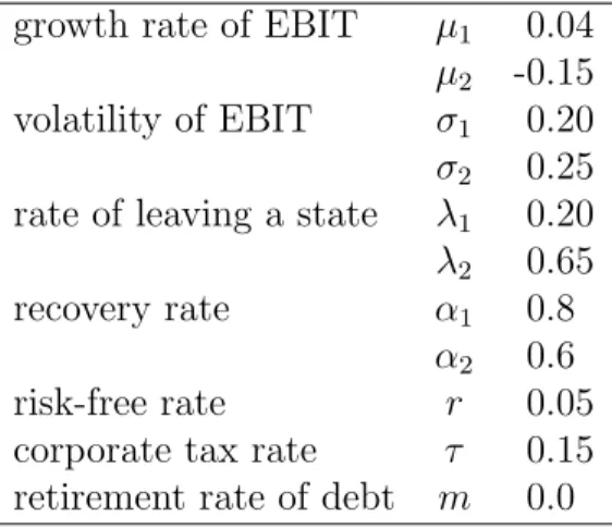
Table 1: Summary of the calibrated parameters used in the benchmark case. The parameters are estimated on aggregated S&P500 date.

growth rate of EBIT µ1 0.04 µ2 -0.15 volatility of EBIT σ1 0.20 σ2 0.25 rate of leaving a state λ1 0.20 λ2 0.65 recovery rate α1 0.8

α2 0.6 risk-free rate r 0.05 corporate tax rate τ 0.15 retirement rate of debt m 0.0

For each i0 we receive an optimal principal P, a fair coupon C, and two distinguishable default thresholds K1 and K2. We denote the solution to (32) with vi∗(x) and define the optimal leverages by l_i∗ = d∗_i(x)/v_i∗(x). There are two different optimal capital structures, one for state one and one for state two.

4

Implications for optimal capital structure

In this section we focus on the structural estimation of the parameters of the model and the implication for corporate financing policies. We call the set of estimated parameters benchmark scenario. Table 1 summarizes the estimated parameters.

4.1

Parameter estimation

The parameters λ1, λ2 that determine the transition of the states of the economy are estimated to fit stylized facts on the state of the US-economy after the 1960ies. An average recession lasts for 5 years4 _{which corresponds to λ}

1 = 0.2. Being currently in an expansion, then the probability of entering a recession within one year is about 18% and within two

4_{The average length of stateiis given by 1/λ}

years 33%5_{. We choose a conservative setting by assuming that the average length of a} recessions is much shorter and set the rate of leaving the recession to λ2 = 0.65. In this manner a recession lasts on average for 1.54 years and the probablility of leaving a recession within one year is 48% and 73% within two years. In the long run about 76% of time is spend in an expansion an 24% in a contraction. Firms’ EBIT follows the positive drift on average longer than the negative one.

We calibrate the EBIT-process xt to fit the annually aggregated EBIT of S&P500 firms. We do not use firm level data for calibration because the difference in trends across the business cycle is more pronounced in aggregated data. An observation year is regarded to be a recession if at least six month of the fiscal year is considered as a recession by the monthly NBER recession indicator. Otherwise, the year belongs to an expansion. Using annual Compustat data from 1962 to 2006, we observe a positive average growth rate of the aggregated S&P500 EBIT in expansions and a negative growth rate in recessions. Due to our assumption that investors are risk neutral, we choose µ1 = 0.04 and µ2 = −0.15. Uncertainty in form of a volatility is intuitively higher in recessions. We choose σ1 = 0.2 and σ2 = 0.25. We set the initial level of EBIT to the arbitrary value x0 = 10. All results in percent, especially the optimal leverage ratios and the benefit to leverage, do not vary inx0. In line with Gilson (1997) and Andrade and Kaplan (1998) who report defaults costs of 20% to 40 %, we choose a recovery rate in an expansion of α1 = 0.80 and in a recession α2 = 0.60. In line with previous research we set the corporate tax rate τ to 15% and the risk free rate of interest r to 0.05 approximating the historical average of a short term US government bond.

Figure 1 shows the path of aggregated S&P 500 EBIT. The graph displays the stylized facts of the regime switching process. During expansions there is a positive growth in EBIT while in recession the growth rate is negative. Without the regime switching ability it is not possible to characterize certain periods as recessions. The possibility of increasing and

5_{The cumulative distribution function of the exponential distrubutionF}

exp(t) gives the probability that

Figure 1: Aggregated EBIT of S&P500 firms from 1975 to 2001. Recession years classified by NBER are 1981-1982, 1990-1991, and 2001.

decreasing EBIT would be constant throughout time and independent of the business cycle.

4.2

Pro-cyclical leverage and benefits

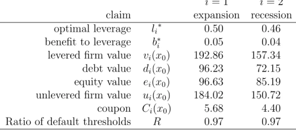
The results of our benchmark scenario in table 2 show that optimal leverage is pro-cyclical. In expansions the firm chooses to finance 50% of their capital needs with debt and 50% to be equity. The positive growth of EBIT last on average 60 month which pushes EBIT on average further away from the default thresholds and reduces default. When after an average expansion a state switch to a recession occurs, then, despite the negative EBIT growth, default is unlikely because the distance between EBIT xt and the default threshold K2 has increased during the expansion. In contrast, if the present state is already a recession, then the firm chooses an optimal leverage ratio of 46%. On average EBIT loses 15% continuously within one year, which leads to lower debt capacity and interest coverage. Management chooses to finance a larger fraction with equity because additonal debt would increase default risk and reduce the levered firm value.

is increased through debt issuance of 96.23 by 5%. These benefits are obtained in two ways. First, in the present expansion the firm generates high tax shields and second, when the next recession enters, the firm has the same amount of debt outstanding but on average at a higher EBIT level. In this manner the tax benefits remain high in the upcoming recession. In contrast, if the present state is already a recession, the unlevered asset value of 157.34 is increased through the debt issuance of 72.15 only by 4%. Now, the firm cannot afford operating at a high leverage ratio and misses tax benefits compared to an expansion. As the expansion sets in tax benefits become more secure but are much lower compared to those that could be generated if the present state was already an expansion. Our values roughly reflect the estimates of benefits to leverage by Graham (2000). Figure 2a shows the levered firm value in dependence of the chosen leverage. First the levered firm value increase in both states due to rising tax benefits. At some point the marginal default costs exceed the additional tax benefits leading to negative net benefits which result in a decreasing firm value. The point where marginal default costs exceed marginal tax benefits is smaller in a recession leading to the observed pro-cyclical leverage. The choice of operating at a lower leverage ratio reflects a more conservative financial policy.

As long as managers choose a principal where the levered firm value exceeds the unlevered firm value, they create (not necessarily optimal) shareholder value. The points where the solid and the dashed line hit the dotted lines, are the barrier to the region where managers destroy shareholder value, because the levered firm is smaller than its unlevered value. This barrier is pro-cyclical, i.e. in an expansion this point is reached at an leverage of 0.81 and in an recession at 0.74. Because of the positive growth expectations of EBIT in expansions, the levered firm value still exceeds the unlevered value at a higher leverage level.

The value of equity is counter-cyclical. This does not imply a higher value for shareholders in recessions, it rather reflects the choice of financial sources. In our model the costs of choosing equity financing are lower, but on the other hand there are no benefits in form of tax shields. The change in shareholders’ wealth is reflected through the unlevered firm value

Table 2: Results on state dependent capital structure using the parameters from the benchmark scenario.

i= 1 i= 2 claim expansion recession optimal leverage li∗ 0.50 0.46 benefit to leverage b∗_i 0.05 0.04 levered firm value vi(x0) 192.86 157.34 debt value di(x0) 96.23 72.15 equity value ei(x0) 96.63 85.19 unlevered firm value ui(x0) 184.02 150.72 coupon Ci(x0) 5.68 4.40 Ratio of default thresholds R 0.97 0.97

and the change in benefits to leverage.

The default thresholdsKi are counter-cyclical as well. Firms default earlier in a recession than in an expansion due to the negative expected growth rate µ2. In contrast, if a firm operates in an expansion at a EBIT level between the two thresholds, it will remain active because of the expected positive growth of EBIT over time. If a sudden state switch occurs, then all firms with EBIT in the range of [K1, K2] are liquidated simultaneously, which refers to the default clustering described by Driessen (2005), Cremers, Driessen, and Maenout (2008), and Hackbarth, Miao, and Morellec (2006). The counter-cyclical default thresholds follow from the solution to equation (31) and are observed without initial split up into three regions in section 2.

Our theoretical implications explain various empirical findings on corporate capital struc-ture. Korteweg (2010) calculates optimal leverage with help of an extended Modigliani and Miller (1958) setting and observes pro-cyclical leverage ratios and benefits. His empirically estimated benefits are lower than our predicted values, because our optimal leverage ratios are based on a risk-neutral setting. Covas and Den Haan (2010) find that debt issuances are pro-cyclical for most size-sorted US-firms. In contrast, Korajczyk and Levy (2003) state that leverage ratios are counter-cyclical. These findings do not contradict each other, be-cause Korajczyk and Levy (2003) examine observed leverage ratios which do not correspond to optimal or target leverage ratios because of market frictions (Leary and Roberts (2005)).

Retained earnings and temporary earnings shock change leverage ratios over time and the costs of returning to the optimum might exceed the benefits. In our model at the end of an expansion a firm operates at a leverage ratio that is substantially lower than the optimal recession-leverage due to the increased EBIT level. Hence, observed leverage ratios appear to be counter-cyclical while optimal leverage ratios remain pro-cyclical.

In other parsimonious trade-off models of capital structure (Hackbarth, Miao, and Morel-lec (2006)) optimal leverage is counter-cyclical. Their result is mainly driven by their assumed EBIT-process that is discontinuous at turning points. Their proposed EBIT process looses a fraction of its value in recession, but is restored to the old level in the next expansion. Implicitly the expected growth rate of EBIT in a recession is large because investors expect a positive jump. As well, in their model the growth rate in expansion is negative, because of the probability to a switch to a recession. In line with Nieuwerburgh and Veldkamp (2006) we model a “sharp and short” downturn and a “more gradual” resumption of the expansion to obtain a realistic setting.

4.3

Cost of being over- or underlevered

In this section we show that costs of operating at a non-optimal leverage are higher in recessions and that capital structure adjustments due to these costs are more common around turning points of the economy.

Often managers face the problem that they cannot infer the growth rate of their firm’s EBIT exactly, nor do they know the present state with certainty. If they choose a leverage ratio based on an estimate that might deviate from the true value, they come to the problem of operating at a non-optimal leverage. For example, if the manager believes that the present state is an expansion, but in reality a recession has already started, then his chosen principal exceeds the optimal value. In this case the firm would be overlevered and face higher default costs. In contrast, if the firm chooses a principal that is too small, i.e. it underestimates its growth rate, the firm is underlevered and misses substantial tax benefits. In both cases the

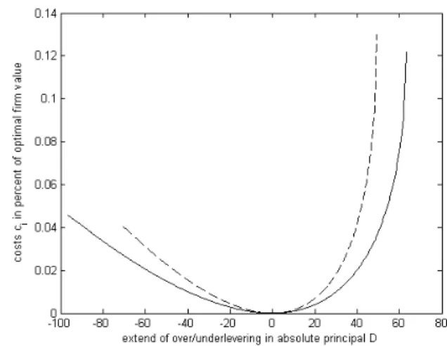
(a) leverage and levered firm value (b) costs of being over- or underlevered

Figure 2: Panel (a) shows the levered firm value in dependence of chosen leverage. All parameters corre-spond to the values in table 1. The solid line is the levered firm value in a expansion (i= 1), the dashed line in a recession (i= 2). The upper dotted line is the unlevered firm value in an expansion and the lower dotted line the unlevered firm value in a recession. The optimal levered firm values are marked with a circle. Panel (b) shows the costs of being over- or underlevered. The x-axis is the deviationDof the chosen principal from the optimal leverage in the corresponding state. The cost of being over- or underleveredci(D) are measured

as difference between the optimal and the chosen levered firm value in percent. The solid lines are the cost in an expansion and the dashed line in a recession.

levered firm value is smaller than the optimum.

We measure the costs of being over- or underlevered ci as the loss in the levered firm value as percentage of optimal valuev∗_i and dependent on the present state i= 1,2. In this context we regard the levered firm valuevi as a function of the (non-optimal) principalP and define the difference between chosen principal P and optimal principalP∗ as D =P −P∗. Initial EBIT x0 are treated as a constant parameter of the levered firm value. We can now write the costs of being over- or underlevered ci(D) as

ci(D) = 1−

vi(P∗+D) vi(P∗)

. (33)

Figure 2b plots the costsci against the difference in principalsDfor both statesi. ForD= 0 the firm incurs no additional costs. If the principal is too low, i.e. D < 0, the firm faces costs of being underlevered due to missing tax benefits because the tax deductible coupon payments are lower than they are in the optimal case. These costs are higher in recessions

since expected future earnings decrease on average and other means of creating shareholder value become more important. The costs of being underlevered are limited to maximum benefits to leverage.

For D > 0 the firm faces costs of being overlevered. Beyond the optimal principal marginal default costs increase more rapidly than tax benefits due to the high default proba-bility. The difference in growth rates across the business cycle leads to higher costs of being overlevered in recessions. The loss of shareholder value is in this case not limited to the tax benefits because a very high leverage can diminish the levered value to the liquidation value of the assets. Combining our results, our model shows that in recessions it is more important to operate at the optimal leverage because additional costs can reduce the shareholder value more heavily.

For a small deviation from the optimum the costs do not exceed a high percentage of the levered firm value. For example, adjustment costs for debt-equity swaps to return to the optimum might outweigh the benefits. If adjustment costs are smaller than 1% of the levered firm value, then a deviation of -40 or +30 units of debt would be still be less costly than adjusting to the optimum. Hence, firms do not tend to adjust their leverage often as long as a state switch does not occur and the optimum remains the same. In contrast, if a state switch occures then the optimal principal moves by about 24 units. Especially a switch from an expanison to a recession leads to costs of overlevering, because the optimal principal is reduced by those 24 units. Now, the costs of being overlevered can exceed some percentage points of the levered firm value and it would be optimal to adjust to the target leverage. Therefore, leverage adjustments should be more common around turning points than within a state of the business cycle. Since costs of being overlevered are higher in recessions, adjustments are more likely in this state of the economy than in expansions. Our theoretical results establish empirically testable implications on the timing of capital structure adjustments.

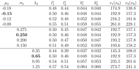
Table 3: Results on the parameter estimation for changing macroeconomic conditions. All parameters but

µ2, σ2, and λ2 are held constant to the values of the benchmark scenario. The bold number indicate the

benchmark scenario. µ2 σ2 λ2 l1∗ l ∗ 2 b ∗ 1 b ∗ 2 v1(x0) v2(x0) -0.18 0.48 0.44 0.044 0.040 174.9 138.8 -0.15 0.50 0.46 0.048 0.044 192.9 157.3 -0.12 0.52 0.48 0.052 0.048 216.2 181.6 -0.08 0.55 0.51 0.059 0.055 261.0 228.1 0.275 0.50 0.45 0.047 0.042 192.7 157.1 0.250 0.50 0.46 0.048 0.044 192.9 157.3 0.200 0.50 0.47 0.050 0.047 193.2 157.8 0.150 0.51 0.49 0.052 0.050 193.6 158.2 0.35 0.44 0.39 0.037 0.032 145.3 108.0 0.65 0.50 0.46 0.048 0.044 192.9 157.3 0.95 0.54 0.51 0.057 0.053 235.5 201.6 1.25 0.57 0.54 0.064 0.060 273.7 241.4

4.4

Changes in macroeconomic risk

As noted by Stock and Watson (2002) macroeconomic risk has changed over time. A shift in macroeconomic conditions influences the market value of corporate debt and equity because it strongly affects the default risk. In our model there are three ways to reflect macroeconomic risk: the size of the negative growth rate µ2, the volatility of EBIT in recessions σ2 and the rate of leaving a recession λ2.

First, we analyze the impact of the growth rate in contractions on optimal leverage and the benefit to leverage. Table 3 shows the results of a variation inµ2 from -0.18 to -0.03. As macroeconomic risk decreases, the optimal leverage ratios increase by 7% and benefits rise by 1.5% in both states. The effect of a changing growth rate is reflected the strongest in the levered firm value which rises by 50% and is driven by an increase of the unlevered asset value that rises due to the change in µ2. The firm responds to lower risk with an increase in leverage that comes with the trade-off of a higher default probability. In comparison to the levered firm value the change in benefits to leverage is only marginal.

As a second approach, we focus on the effect of a change in the EBIT volatility. σ2reflects the deviation from the downtrend of EBIT and is twofold. The chances of achieving high

EBIT levels increase at the cost of a higher default probability. The results of our parameter variation in table 3 yield that the downside risk is larger because the firm operates at a lower leverage ratio for high values of σ2. The decline in the optimal leverage ratio in recessions is more sharply than in expansions because a present recession influences the valuation stronger than future recessions due to discounting of cash flows. The benefit to leverage decreases slightly from 5.2% (5%) to 4.7% (4.2%) as volatility increases because the firm is less likely to benefit from future tax shields. In contrast, the levered firm value is almost unaffected by an increase in σ2 which indicates that the change in the tax shield and in the default costs are of equal magnitude. As shown in equation (8), the unlevered firm value is independent of σ2 and constant in the parameter variation.

The third factor that characterizes a recession is the expected length of the state which equals the inverse of the rate of leaving state twoλ2. The length of a contraction determines the time during which the EBIT is exposed to the negative growth rate µ2. Our results yield that a short recession (i.e. a high rate of leaving a recession) results in higher optimal leverage ratios (0.57 and 0.54). In case of a long recession the optimal ratios are much lower (0.44 and 0.39). The levered firm value is strongly affected by the length of a recession and so are the benefits to leverage that almost double.

Combining the results of the three parameter variations, we find that a reduction in macroeconomic risk increases optimal leverage. By acting optimally firms can achieve similar benefits by adjusting their financial policy to the new conditions. Shareholders profit primary through the increase in the unlevered firm value, but not through the benefits to debt financing which remain almost equal. Applying this finding to corporate financing policies, we conclude that after the observed change of macroeconomic risk in the 1980s, debt became more attractive to firms because the default risk was reduced. Speaking empirically, optimal leverage ratio should be higher after the change in the macroeconomic risk.

5

Concluding remarks

Our study shows that macroeconomic conditions are an important determinant of capital structure decisions. Optimal leverage and benefits to leverage depend on the present state of the economy and on the additional risk of a sudden switch to the other state. Optimal leverage ratios and benefits to leverage vary pro-cyclically, i.e. they are higher in expansions, because of varying growth rates of EBIT. Even though debt becomes more risky in recessions, tax benefits remain an important mean to maximize the levered firm value.

A change in macroeconomic risk, such as milder or less volatile recessions, leads to an increase of the levered firm value and the optimal leverage ratios. However, benefits to leverage increase only a little. Hence, after the change in macroeconomic risk in the 1980s, firm values and leverage ratios should have gone up, but firms should not have profited much from increasing tax benefits.

Our model shows that being over- or underlevered is more costly in recessions and that capital structure adjustments due to these costs are more common in recessions or around turning points. If a firm has problems to determine its optimal capital structure exactly, then the firm should act more conservatively and issue less debt. The costs of the lower tax shield are smaller than possible high default costs.

Our static setting can be extended to a dynamic setting, that would give the firm the option of restructuring its capital if EBIT have reached an upper threshold. However, the results of Hackbarth, Miao, and Morellec (2006) and Bhamra, Kuehn, and Strebulaev (2009) indicate that dynamics in structural models do not change the order of the results, only the level of leverage. Hackbarth, Miao, and Morellec (2006) find that optimal leverage is smaller when the firm has the option to issue debt in the future, but the cyclicality of debt issuances remains. In our model we omit the option of future debt issuance to keep the model parsimonious.

References

Andrade, G., and S. Kaplan (1998): “How Costly Is Financial (Not Economic)

Dis-tress? Evidence from Highly Leveraged Transactions That Became Distressed,” Journal of Finance, 53, 1443–1493.

Bhamra, H. S., L.-A. Kuehn,andI. A. Strebulaev(2009): “The Aggregate Dynamics

of Capital Structure and Macroeconomic Risk,” Review of Financial Studies, 23(2).

Chen, H.(2010): “Macroeconomic Conditions and the Puzzles of Credit Spreads and

Cap-ital Structure,”Journal of Finance, 65, 2171–2212.

Covas, F., and W. J. Den Haan (2010): “The Cyclical Behavior of Debt and Equity

Finance,”American Economic Review, Forthcoming.

Cremers, M., J. Driessen, and P. Maenout (2008): “Explaining the Level of Credit

Spreads: Option-Implied Jump Risk Premia in a Firm Value Model,”Review of Financial Studies, 21, 2209–2242.

Driessen, J.(2005): “Is Default event risk priced in corporate bonds?,”Review of Financial

Studies, 18, 165–195.

Driffill, J., M. Raybaudi, and M. Sola (2003): “Investment under uncertainty with

stochastically switching Profit Streams,”Studies in Nonlinear Dynamics & Econometrics, 7(1), 1–38.

Gilson, S. (1997): “Transaction Costs and Capital Structure Choice: Evidence from

Fi-nancially Distressed Firms,”Journal of Finance, 52, 161–196.

Goldstein, R., N. Ju, and H. E. Leland(2001): “An EBIT-Based Model of Dynamic

Capital Structure,” The Journal of Business, 74(4), 483–512.

Graham, J. R. (2000): “How Big Are the Tax Benefits of Debt,” Journal of Finance, 55,

Guo, X. (2001): “Information and option pricings,” Quantitive Finance, 1, 38–44.

Hackbarth, D., J. Miao, and E. Morellec (2006): “Capital Structure, Credit Risk,

and Macroeconomic Conditions,”Journal of Financial Economics, 82(3), 519–550.

Korajczyk, R., and A. Levy (2003): “Capital structure choice: macroeconomic

condi-tions and financial constraints,”Journal of Financial Economics, 68, 75–109.

Korteweg, A.(2010): “The Net Benefits to Leverage,”Journal of Finance, 65, 2137–2170. Leary, M., and M. Roberts (2005): “Do firms rebalance their capital structures?,”

Journal of Finance, 60, 2575–2619.

Leland, H. E. (1994): “Corporate Debt Value Bond Covenants and Optimal Capital

Structure,”Journal of Finance, 49(4), 1213–1252.

(1998): “Agency Costs, Risk Management, and Capital Structure,” The Journal of Finance, 53, 1213–1243.

Leland, H. E., and K. B. Toft (1996): “Optimal Capital Structure, Endogenous

Bankruptcy, and the Term Structure of Credit Spreads,” The Journal of Finance, 51(3), 987–1019.

Mello, A., and J. Parsons (1992): “Measuring the agency cost of debt,” Journal of

Finance, 47(5), 1887–1904.

Modigliani, F., and M. Miller(1958): “The Cost of Capital, Corporation Finance, and

the Theory of Investment,” American Economic Review, 48, 261–297.

Nieuwerburgh, S. V.,andL. Veldkamp(2006): “Learning asymmetries in real business

cycles,” Journal of Monetary Economics, 53(4), 753–772.

Stock, J., and M. Watson (2002): “Has the Business Cycled Changed and Why?,”

A

Appendix

A.1

Derivation of the differential equations in section

The derivation of the differential equations for the levered firm, the unlevered firm, and debt value follows Driffill, Raybaudi, and Sola (2003). First, we regard the unlevered firm value ut = u(xt) of the firm which corresponds to the value of a firm that does not issue any debt. Let _E denote the expectation operator on the σ-algebra that is generated by the Brownian motion and the Markov chain, and _EW denotes the expectation operator on the σ-algebra of just the Brownian motion. The infinitesimal change of its value can be described by the following equation:

rut dt = (1−τ)xt dt+E[dut] . (34)

Since all investors are risk neutral, all cash flows are discounted at the risk free rate r. The required rate of returnrequals the growth of after tax EBIT (1−τ)xtplus the change in its value_E[du] that arises because of a variation ofxtand a possible state switch. Letui denote the unlevered asset value conditioned on the statei. We assume that the present state is 1, so i= 1. With the transition probabilityλ1 we have

E[ut+dt] = (1−λ1dt)EW[u1(xt+dt)] +λ1dt EW[u2(xt+dt)]. (35)

The first summand denotes the event of remaining in state 1 times its probability, and the second part is the case of switching to state 2. The expected change of U on the interval dt

is

E[du] =E[u(xt+dt)−u(xt)]

= (1−λ1dt) EW[u1(xt+dt)] +λ1dt EW[u2(xt+dt)]−EW[u1(xt)]

=_EW[u1(xt+dt)−u1(xt)] +λ1dt EW[u2(xt+dt)−u1(xt+dt)] (36)

The second summand describes a switch from state one to state two and is independent of the expectation operator_EW. The first part equals the change of u given that the economy remains in the first state. Under the assumption of remaining in state onextis an Itˆo-process, so that we can apply Itˆo’s lemma to u1(xt) and receive

du1 = µ1xu01+ 1 2σ 2_x2_u00 1 dt+σ1xu01 dWt . (37)

It holds that _EW(σ1x dWt) = 0 and we receive

E[du] = µ1xu01 + 1 2σ 2 1x 2_u00 1 dt+λ1(u2−u1) dt . (38)

Using (38), equation (34) equals

ru dt = (1−τ)x dt+ µ1xu01+ 1 2σ 2 1x 2 u00₁ dt+λ1(u2−u1) dt . (39)

Hence, the differential equation to determine u1 is

1 2x

2

σ₁2u00₁ +µ1xu01−ru1 +λ1(u2−u1) + (1−τ)x= 0 . (5)

If we assume that the present state is 2, the same application of Itˆo’s lemma yields

1 2x

2

(5) and (6) form a system of ordinary differential equations that describe the liquidation value of the firm.

In order to derive differential equations for the value of corporate debt and the levered firm, one needs to substitute the continuous payment (1−τ)x in (34) by C +mP or (1− τ)x+τ C, respectively.

In the case of corporate debt value di(x) the firm defaults in state 2 but remains active in state 1 if K1 < xt< K2. (35) reads in this case:

E[dt+dt] = (1−λ1dt) EW[d1(xt+dt)] +λ1dt EW[α2u2(xt+dt)], (40)

where α2 is the recovery rate in state 2. With this modification one can derive differential equations for the transient region by applying the same exercise as above.

A.2

Solving the differential equations

We will consider the case of corporate debt only. In the transient region we have to solve equation (11): 1 2x 2_σ2 1d 00 1 +µ1xd01−(r+m)d1+λ1(α2w2x−d1) +C+mP = 0 (11)

which is a linear ordinary differential equation of second order. The homogeneous part of the solution reads

dhom₁ (x) = A1xγ 1

+A2xγ 2

where γi are the roots of the characteristic equation of the equivalent differential equation with constant coefficients. γi satisfies

γ1,2 = 0.5− µ1 σ2 1 ± s 0.5− µ1 σ2 1 2 + 2r+m+λ1 σ2 1 . (42)

The particular solution of (11) reads

dpart₁ (x) = C+mP

r+m+λ1

+ α2λ1w2x

r+m+λ1−µ1

. (43)

w2 is the constant coefficient for the function for the value of unlevered assetsui(x) = wix. Combined, we have a function with two unknown coefficients A1 and A2:

d1(x) = A1xγ1 +A2xγ2 + C+mP r+m+λ1 + α2λ1w2x r+m+λ1−µ1 (44)

In the action region the system of differential equations (12) and (13)

1 2x 2_σ2 1d 00 1 +µ1xd01−(r+m)d1+λ1(d2 −d1) +C+mP = 0 (12) 1 2x 2_σ2 2d 00 2 +µ2xd02−(r+m)d2+λ2(d1 −d2) +C+mP = 0 (13)

is linear and of second order as well. By transforming the equations to a system with constant coefficients, one obtains the homogeneous solution functions

dhom₁ (x) =A3xβ1 +A4xβ2 +A7xβ3 +A8xβ4 , (45)

βi are the four distinct roots of the fourth order polynomial det          −β 1 0 0 −a1 1−a4−β −a3 0 0 0 −β 1 −a6 0 −a2 1−a5−β          = 0 (47) where a1 = −2(r+m)−2λ1 σ2 1 a2 = −2(r+m)−2λ2 σ2 2 a3 = 2_σλ21 1 a4 = 2_σµ21 1 a5 = 2_σµ22 2 a6 = 2_σλ22 2 (48)

that have to be calculated numerically. The particular solutions to (12) and (13) read

dpart_i (x) = C+mP

r+m i= 1,2. (49)

Combining (45), (45), and (49), the general solution functions have eight unknown coeffi-cients: d1(x) = A3xβ1 +A4xβ2 +A7xβ3 +A8xβ4 + C+mP r+m (50) d2(x) = A5xβ1 +A6xβ2 +A9xβ3 +A10xβ4 + C+mP r+m (51)

In line with Driffill, Raybaudi, and Sola (2003) we find that β1, β2<0 and β3, β4>0. Since the solution functions are bounded by the value of risk-free debt C_r+₊mP_m , it follows that

A7 = A8 = A9 = A10 = 0. Combining (44), (50), and (51) there are six coefficients left A1, A2, A3, A4, A5, A6 to be determined.

For every pair of real numbersAj,Ai there is another numberbj that satisfiesbjAj =Ai. In our case we can determine bj independent of x and hence constant for a given set of parameters. Assuming b5A5 = A3 and b6A6 = b4 and plugging (50) and (51) into the

differential equation (12) leads to b5 =− 1 λ1 1 2σ 2 1β1(β1−1) +µ1β1−(r+m)−λ1 (52) b6 =− 1 λ1 1 2σ 2 1β2(β2−1) +µ1β2−(r+m)−λ1 (53)

Now, there are four unknown coefficients left that can be determined uniquely with the boundary conditions (14) - (17).

When deriving the solutions for the value of the levered firm vi(x), one needs to set m = 0 and use the boundary conditions (23) - (26). The coefficients of the terms with positive exponents equal to zero because the levered firm value is bounded by wix+τ C. ˆβi and ˆγi correspond to βi and γi with m= 0, i= 1,2.

CFR Working Paper Series

Centre for Financial Research Cologne

CFR Working Papers are available for download from www.cfr-cologne.de. Hardcopies can be ordered from: Centre for Financial Research (CFR), Albertus Magnus Platz, 50923 Koeln, Germany.

2011

No. Author(s) Title

11-12 D. Hess, P. Immenkötter Optimal Leverage, its Benefits, and the Business Cycle

11-11 N. Heinrichs, D. Hess,

C. Homburg, M. Lorenz, S. Sievers

Extended Dividend, Cash Flow and Residual Income Valuation Models – Accounting for Deviations from Ideal Conditions

11-10 A. Kempf, O. Korn,

S. Saßning Portfolio Optimization using Forward - Looking Information

11-09 V. Agarwal, S. Ray Determinants and Implications of Fee Changes in the Hedge

Fund Industry

11-08 G. Cici, L.-F. Palacios On the Use of Options by Mutual Funds: Do They Know What

They Are Doing?

11-07 V. Agarwal, G. D. Gay,

L. Ling

Window Dressing in Mutual Funds

11-06 N. Hautsch, D. Hess,

D. Veredas The Impact of Macroeconomic News on Quote Adjustments, Noise, and Informational Volatility

11-05 G. Cici The Prevalence of the Disposition Effect in Mutual Funds'

Trades

11-04 S. Jank Mutual Fund Flows, Expected Returns and the Real Economy

11-03 G.Fellner, E.Theissen Short Sale Constraints, Divergence of Opinion and Asset

Value: Evidence from the Laboratory

11-02 S.Jank Are There Disadvantaged Clienteles in Mutual Funds?

11-01 V. Agarwal, C. Meneghetti The Role of Hedge Funds as Primary Lenders

2010

No. Author(s) Title

10-20 G. Cici, S. Gibson,

J.J. Merrick Jr.

Missing the Marks? Dispersion in Corporate Bond Valuations Across Mutual Funds

10-19 J. Hengelbrock,

E. Theissen, C. Westheide Market Response to Investor Sentiment

10-17 D. Hess, D. Kreutzmann, O. Pucker

Projected Earnings Accuracy and the Profitability of Stock Recommendations

10-16 S. Jank, M. Wedow Sturm und Drang in Money Market Funds: When Money

Market Funds Cease to Be Narrow

10-15 G. Cici, A. Kempf, A.

Puetz Caught in the Act: How Hedge Funds Manipulate their Equity Positions

10-14 J. Grammig, S. Jank Creative Destruction and Asset Prices

10-13 S. Jank, M. Wedow Purchase and Redemption Decisions of Mutual Fund

Investors and the Role of Fund Families

10-12 S. Artmann, P. Finter,

A. Kempf, S. Koch, E. Theissen

The Cross-Section of German Stock Returns: New Data and New Evidence

10-11 M. Chesney, A. Kempf The Value of Tradeability

10-10 S. Frey, P. Herbst The Influence of Buy-side Analysts on

Mutual Fund Trading

10-09 V. Agarwal, W. Jiang,

Y. Tang, B. Yang Uncovering Hedge Fund Skill from the Portfolio Holdings They Hide

10-08 V. Agarwal, V. Fos,

W. Jiang Inferring Reporting Biases in Hedge Fund Databases from Hedge Fund Equity Holdings

10-07 V. Agarwal, G. Bakshi,

J. Huij Do Higher-Moment Equity Risks Explain Hedge Fund Returns?

10-06 J. Grammig, F. J. Peter Tell-Tale Tails

10-05 K. Drachter, A. Kempf Höhe, Struktur und Determinanten der Managervergütung-

Eine Analyse der Fondsbranche in Deutschland

10-04 J. Fang, A. Kempf,

M. Trapp Fund Manager Allocation

10-03 P. Finter, A.

Niessen-Ruenzi, S. Ruenzi The Impact of Investor Sentiment on the German Stock Market

10-02 D. Hunter, E. Kandel,

S. Kandel, R. Wermers Endogenous Benchmarks

10-01 S. Artmann, P. Finter,

A. Kempf

Determinants of Expected Stock Returns: Large Sample Evidence from the German Market

2009

No. Author(s) Title

09-17 E. Theissen Price Discovery in Spot and Futures Markets:

A Reconsideration

09-16 M. Trapp Trading the Bond-CDS Basis – The Role of Credit Risk

and Liquidity

09-14 A. Kempf, O. Korn,

M. Uhrig-Homburg

The Term Structure of Illiquidity Premia

09-13 W. Bühler, M. Trapp Time-Varying Credit Risk and Liquidity Premia in Bond and

CDS Markets

09-12 W. Bühler, M. Trapp Explaining the Bond-CDS Basis – The Role of Credit Risk and

09-11 S. J. Taylor, P. K. Yadav,

Y. Zhang Cross-sectional analysis of risk-neutral skewness

09-10 A. Kempf, C. Merkle,

A. Niessen Low Risk and High Return - How Emotions Shape Expectations on the Stock Market

09-09 V. Fotak, V. Raman,

P. K. Yadav

Naked Short Selling: The Emperor`s New Clothes?

09-08 F. Bardong, S.M. Bartram,

P.K. Yadav Informed Trading, Information Asymmetry and Pricing of Information Risk: Empirical Evidence from the NYSE

09-07 S. J. Taylor , P. K. Yadav,

Y. Zhang

The information content of implied volatilities and model-free volatility expectations: Evidence from options written on individual stocks

09-06 S. Frey, P. Sandas The Impact of Iceberg Orders in Limit Order Books

09-05 H. Beltran-Lopez, P. Giot,

J. Grammig Commonalities in the Order Book

09-04 J. Fang, S. Ruenzi Rapid Trading bei deutschen Aktienfonds:

Evidenz aus einer großen deutschen Fondsgesellschaft

09-03 A. Banegas, B. Gillen,

A. Timmermann, R. Wermers

The Performance of European Equity Mutual Funds

09-02 J. Grammig, A. Schrimpf,

M. Schuppli Long-Horizon Consumption Risk and the Cross-Section of Returns: New Tests and International Evidence

09-01 O. Korn, P. Koziol The Term Structure of Currency Hedge Ratios

2008

No. Author(s) Title

08-12 U. Bonenkamp,

C. Homburg, A. Kempf Fundamental Information in Technical Trading Strategies

08-11 O. Korn Risk Management with Default-risky Forwards

08-10 J. Grammig, F.J. Peter International Price Discovery in the Presence

of Market Microstructure Effects

08-09 C. M. Kuhnen, A. Niessen Public Opinion and Executive Compensation

08-08 A. Pütz, S. Ruenzi Overconfidence among Professional Investors: Evidence from

Mutual Fund Managers

08-07 P. Osthoff What matters to SRI investors?

08-06 A. Betzer, E. Theissen Sooner Or Later: Delays in Trade Reporting by Corporate

Insiders

08-05 P. Linge, E. Theissen Determinanten der Aktionärspräsenz auf

Hauptversammlungen deutscher Aktiengesellschaften

08-04 N. Hautsch, D. Hess,

C. Müller Price Adjustment to News with Uncertain Precision

08-03 D. Hess, H. Huang,

A. Niessen

How Do Commodity Futures Respond to Macroeconomic News?

08-02 R. Chakrabarti,

W. Megginson, P. Yadav Corporate Governance in India

2007

No. Author(s) Title

07-16 M. Bär, A. Niessen,

S. Ruenzi The Impact of Work Group Diversity on Performance: Large Sample Evidence from the Mutual Fund Industry

07-15 A. Niessen, S. Ruenzi Political Connectedness and Firm Performance:

Evidence From Germany

07-14 O. Korn Hedging Price Risk when Payment Dates are Uncertain

07-13 A. Kempf, P. Osthoff SRI Funds: Nomen est Omen

07-12 J. Grammig, E. Theissen,

O. Wuensche Time and Price Impact of a Trade: A Structural Approach

07-11 V. Agarwal, J. R. Kale On the Relative Performance of Multi-Strategy and Funds of

Hedge Funds

07-10 M. Kasch-Haroutounian,

E. Theissen Competition Between Exchanges: Euronext versus Xetra

07-09 V. Agarwal, N. D. Daniel,

N. Y. Naik

Do hedge funds manage their reported returns?

07-08 N. C. Brown, K. D. Wei,

R. Wermers Analyst Recommendations, Mutual Fund Herding, and Overreaction in Stock Prices

07-07 A. Betzer, E. Theissen Insider Trading and Corporate Governance:

The Case of Germany

07-06 V. Agarwal, L. Wang Transaction Costs and Value Premium

07-05 J. Grammig, A. Schrimpf Asset Pricing with a Reference Level of Consumption:

New Evidence from the Cross-Section of Stock Returns

07-04 V. Agarwal, N.M. Boyson,

N.Y. Naik Hedge Funds for retail investors? An examination of hedged mutual funds

07-03 D. Hess, A. Niessen The Early News Catches the Attention:

On the Relative Price Impact of Similar Economic Indicators

07-02 A. Kempf, S. Ruenzi,

T. Thiele Employment Risk, Compensation Incentives and Managerial Risk Taking - Evidence from the Mutual Fund Industry -

07-01 M. Hagemeister, A. Kempf CAPM und erwartete Renditen: Eine Untersuchung auf Basis

der Erwartung von Marktteilnehmern

2006

No. Author(s) Title

06-13 S. Čeljo-Hörhager,

A. Niessen How do Self-fulfilling Prophecies affect Financial Ratings? - An experimental study

06-12 R. Wermers, Y. Wu,

J. Zechner

Portfolio Performance, Discount Dynamics, and the Turnover of Closed-End Fund Managers

06-11 U. v. Lilienfeld-Toal,

S. Ruenzi Why Managers Hold Shares of Their Firm: An Empirical Analysis

06-10 A. Kempf, P. Osthoff The Effect of Socially Responsible Investing on Portfolio

Performance

06-09 R. Wermers, T. Yao,

J. Zhao The Investment Value of Mutual Fund Portfolio Disclosure

06-07 K. Drachter, A. Kempf,

M. Wagner Decision Processes in German Mutual Fund Companies: Evidence from a Telephone Survey

06-06 J.P. Krahnen, F.A.

Schmid, E. Theissen Investment Performance and Market Share: A Study of the German Mutual Fund Industry

06-05 S. Ber, S. Ruenzi On the Usability of Synthetic Measures of Mutual Fund

Net-Flows

06-04 A. Kempf, D. Mayston Liquidity Commonality Beyond Best Prices

06-03 O. Korn, C. Koziol Bond Portfolio Optimization: A Risk-Return Approach

06-02 O. Scaillet, L. Barras, R.

Wermers False Discoveries in Mutual Fund Performance: Measuring Luck in Estimated Alphas

06-01 A. Niessen, S. Ruenzi Sex Matters: Gender Differences in a Professional Setting

2005

No. Author(s) Title

05-16 E. Theissen An Analysis of Private Investors´ Stock Market Return

Forecasts

05-15 T. Foucault, S. Moinas,

E. Theissen Does Anonymity Matter in Electronic Limit Order Markets

05-14 R. Kosowski,

A. Timmermann, R. Wermers, H. White

Can Mutual Fund „Stars“ Really Pick Stocks? New Evidence from a Bootstrap Analysis

05-13 D. Avramov, R. Wermers Investing in Mutual Funds when Returns are Predictable

05-12 K. Griese, A. Kempf Liquiditätsdynamik am deutschen Aktienmarkt

05-11 S. Ber, A. Kempf,

S. Ruenzi Determinanten der Mittelzuflüsse bei deutschen Aktienfonds

05-10 M. Bär, A. Kempf,

S. Ruenzi Is a Team Different From the Sum of Its Parts? Evidence from Mutual Fund Managers

05-09 M. Hoffmann Saving, Investment and the Net Foreign Asset Position

05-08 S. Ruenzi Mutual Fund Growth in Standard and Specialist Market

Segments

05-07 A. Kempf, S. Ruenzi Status Quo Bias and the Number of Alternatives - An Empirical

Illustration from the Mutual Fund Industry

05-06 J. Grammig, E. Theissen Is Best Really Better? Internalization of Orders in an Open

Limit Order Book

05-05 H. Beltran, J. Grammig,

A.J. Menkveld

Understanding the Limit Order Book: Conditioning on Trade Informativeness

05-04 M. Hoffmann Compensating Wages under different Exchange rate Regimes

05-03 M. Hoffmann Fixed versus Flexible Exchange Rates: Evidence from

Deve