University of New Hampshire
University of New Hampshire Scholars' Repository
Master's Theses and Capstones
Student Scholarship
Winter 2011
Parallel volume rendering for large scientific data
Thomas Fogal
University of New Hampshire, Durham
Follow this and additional works at:
https://scholars.unh.edu/thesis
This Thesis is brought to you for free and open access by the Student Scholarship at University of New Hampshire Scholars' Repository. It has been accepted for inclusion in Master's Theses and Capstones by an authorized administrator of University of New Hampshire Scholars' Repository. For more information, please [email protected].
Recommended Citation
Fogal, Thomas, "Parallel volume rendering for large scientific data" (2011).Master's Theses and Capstones. 684.
PARALLEL VOLUME R E N D E R I N G F O R LARGE
SCIENTIFIC DATA
BY
Thomas Fogal
B.S., University of New Hampshire (2006)
THESIS
Submitted to the University of New Hampshire in Partial Fulfillment of
the Requirements for the Degree of
Master of Science in
Computer Science
UMI Number: 1507822
All rights reserved
INFORMATION TO ALL USERS
The quality of this reproduction is dependent upon the quality of the copy submitted. In the unlikely event that the author did not send a complete manuscript and there are missing pages, these will be noted. Also, if material had to be removed,
a note will indicate the deletion.
UMI
Dissertation Publishing
UMI 1507822
Copyright 2012 by ProQuest LLC.
All rights reserved. This edition of the work is protected against unauthorized copying under Title 17, United States Code.
uest
ProQuest LLC
789 East Eisenhower Parkway P.O. Box 1346
This thesis has been examined and apjiroved
Thesis Director, R. Daniel Bttfgeron Professor of Computer Spfnncc
Philip J. Matcher,
Professor of Computer Science & Chair of the Computer Science Department
Hank R Childs.
Research Professor, Dopatlmeni of Computer Science. University of California, Davis
A C K N O W L E D G M E N T S
The most important 'thank you' has to be for my committee, Professors Bergeron and Hatcher, and Dr. Childs. I think this has dragged on far longer than any of us had anticipated, and developed a scope much larger than intended. Their unending patience and dedication to seeing me through this was a boon when progress was slow and doubts were large. Further, it has been obvious from the start that they have been concerned not simply with the production of another document and another graduate, but the incubation of my much larger professional life during and beyond this thesis. For these things I am forever grateful.
A special acknowledgement should go to Jens Kriiger, who really deserves to be named as part of my committee. He and I developed the volume rendering library "Tuvok", and I must admit he did the heavy lifting in that regard. His advice and help as I implemented the system described here was invaluable, as was his persistent, "So, are you finished yet?" prodding.
Siddharth Shankar deserves special mention as well. Siddharth and I implemented the load balancing aspects mentioned herein, and again most of the credit here belongs to Siddharth.
I am extremely fortunate to have worked on portions of this thesis with the support of the SCI Institute at the University of Utah. I thank the administration there for ensuring that tasks which intersect with my personal motivations and interests flow my way.
Sean Ahem of Oak Ridge National Laboratory provided significant support getting IceT integrated into Visit, and the way Visit accesses multiple GPUs came directly out of conversations he and I had whilst I was at Oak Ridge. The idea of 'decoupled' processing and rendering, which sadly is only mentioned briefly in conclusions due to time constraints,
is entirely his.
I would like to thank Gunther Weber and Mark Howison at LBNL for discussions and guidance during preliminary formulation of our published work related to this thesis.
Paul Navratil at TACC deserves a special 'thanks!'. He helped us get Visit working with Longhorn's GPUs, which was critical in generating the most interesting scalability results presented here. Thanks, Paul!
The CS graduate students at UNH served a very useful role in maintaining my sanity whilst I was there. Thanks, guys. I miss our weekly 'CS socials'.
This research was made possible in part by the Office of Advanced Scientific Comput-ing Research, Office of Science, of the U.S. Department of Energy under Contract No. DE-AC02-05CH11231 through the Scientific Discovery through Advanced Computing (Sci-DAC) program's Visualization and Analytics Center for Enabling Technologies (VACET), by the NIH/NCRR Center for Integrative Biomedical Computing, P41-RR12553-10 and by Award Number R01EB007688 from the National Institute Of Biomedical Imaging And Bioengineering.
Resources were utilized at the Texas Advanced Computing Center (TACC) at the Uni-versity of Texas at Austin and at the National Center for Computational Sciences at Oak Ridge National Laboratory, which is supported by the Office of Science of the U.S. Depart-ment of Energy under Contract No. DE-AC05-00OR22725.
TABLE OF C O N T E N T S
ACKNOWLEDGMENTS Hi LIST OF TABLES vii LIST OF FIGURES viii
1 I N T R O D U C T I O N and R E L A T E D W O R K 1 1.1 Thesis Goals 2 1.2 BACKGROUND 3 2 A R C H I T E C T U R E 6 2.1 Multi-GPU Access 6 2.2 Partitioning 7 2.3 Rendering 9 2.3.1 Tuvok 9 2.3.2 Visit Integration 11 2.4 Compositing 13 3 E V A L U A T I O N 15 3.1 Rendering Times 15 3.2 Memory Strain 18 3.3 Readback and Compositing 20
3.4 Load Balancing 21 3.4.1 Algorithm Details 21
3.4.2 Results 23 3.5 Observations 25
4 S U M M A R Y 27
4.1 Future Work 28
B I B L I O G R A P H Y 29
A P A R A L L E L A P P R O X I M A T E I M A G E C O M P O S I T I O N 30
A.l Parallel Compositing Overview 30 A.2 Expansion of the Over Operator 31
A.3 Significance of Terms 34 A.3.1 Application 36
LIST OF TABLES
2.1 Tuvok Timings 12 3.1 Configuration of GPU clusters utilized 16
LIST OF FIGURES
1-1 Example output of our volume rendering system 3 2-1 Example output of our volume rendering system 7
2-2 Sample volume decomposition 8
2-3 Tuvok Render Modes 10 2-4 Large data sets demonstrating Tuvok 11
3-1 Scalability on Longhorn 17 3-2 Rendering time as a function of brick size 18
3-3 In-core versus out-of-core 19
3-4 Load balancing 22 3-5 Per-process rendering times for the 'Miiller' line given in Figure 3-4. . . 24
A B S T R A C T
PARALLEL V O L U M E R E N D E R I N G F O R L A R G E S C I E N T I F I C DATA
by Thomas Fogal
University of New Hampshire, December, 2011
Data sets of immense size are regularly generated by large scale computing resources. Even among more traditional methods for acquisition of volume data, such as MRI and CT scanners, data which is too large to be effectively visualized on standard workstations is now commonplace.
One solution to this problem is to employ a 'visualization cluster,' a small to medium scale cluster dedicated to performing visualization and analysis of massive data sets gener-ated on larger scale supercomputers. These clusters are designed to fulfill a different need than traditional supercomputers, and therefore their design mandates different hardware choices, such as increased memory, and more recently, graphics processing units (GPUs). While there has been much previous work on distributed memory visualization as well as GPU visualization, there is a relative dearth of algorithms which effectively use GPUs at a large scale in a distributed memory environment. In this work, we study a common visualization technique in a GPU-accelerated, distributed memory setting, and present per-formance characteristics when scaling to extremely large data sets.
CHAPTER 1
INTRODUCTION and RELATED
WORK
Visualization and analysis algorithms, volume rendering in particular, require extensive compute power relative to data set size. One possible solution is to use the large scale supercomputer that generated the data, which clearly has the requisite compute power. But it can be difficult to reserve and obtain the computing resources required for viewing large data sets. An alternative approach, one explored in this paper, is to use a smaller scale cluster equipped with GPUs, which can provide the needed computational power at a fraction of the cost - provided the GPUs can be effectively utilized. As a result, a semi-recent trend has emerged to procure GPU-accelerated visualization clusters dedicated to processing the data generated by high end supercomputers; examples include ORNL's Lens, Argonne's Eureka, TACC's Longhorn, SCI's Tesla-based cluster, and LLNL's Gauss.
Despite this trend, there have been relatively few efforts to study distributed memory, GPU-accelerated visualization algorithms that can effectively utilize the resources available on these clusters. In this paper, we report parallel volume rendering performance charac-teristics on large data sets for a typical machine of this type.
Our system is divided into three stages:
1. An intelligent pre-partitioning which is designed to make combining results from dif-ferent nodes easy.
2. A GPU volume Tenderer to perform the per-frame volume rendering work at interac-tive rates.
3. MPI-based compositing based on a sort-last compositing framework.
Miiller et al. presented a system similar to our own that was limited to smaller data sets [24]. We have extended the ideas in that system to allow for larger data sets, by removing the restriction that a data set must fit in the combined texture memory of the GPU cluster and adding the ability to mix in CPU-based Tenderers, enabling us to analyze parallel performance on extremely large data sets. The primary contribution of this paper is an increased understanding of the performance characteristics of a distributed memory GPU-accelerated volume rendering algorithm at a scale (256 GPUs) much larger than previously published. Further, the results presented here (data sets up to 81923 voxels) represent some
of the largest parallel volume renderings attempted thus far.
1.1 Thesis Goals
Our system and benchmarks allow us to explore issues such as:
• the balance between rendering and compositing, which is a well-studied issue with CPU-based rendering, but previously had unclear performance tradeoffs for rendering on GPU clusters;
• the overhead of transferring data to and from a GPU; • the importance of process-level load balancing; and
• the viability of GPU clusters for rendering very large data.
The rest of this thesis is organized as follows: in Section 1.2, we overview previous work in parallel compositing and GPU volume rendering. In Chapter 2 we outline our system in detail. Chapter 3 discusses our benchmarks and presents their results before drawing
Figure 1-1: Output of our volume rendering system with a data set representing a burning helium flame.
conclusions based on our findings. Appendix A discusses the beginnings of a compositing idea which could not be developed within the constraints of this thesis.
1.2 B A C K G R O U N D
Volume rendering in a serial context has been studied for many years. The basic algo-rithm [7] was improved significantly by including empty space skipping and early ray termi-nation [16]. Max provides one of the earliest formal presentations of the complete volume rendering equation in [21]. Despite significant algorithmic advances from research such as [16], the largest increase in performance for desktop volume Tenderers has come from taking advantage of the 3D texturing capabilities [2,6,31] and programmable shaders [14]
available on modern graphics hardware.
Extensive research has been done on parallel rendering and parallel volume rendering. Much of this work has focused on achieving acceptable compositing times on large systems. Molnar et al. conveyed the theoretical underpinnings of parallel rendering performance [22]. Earlier systems for parallel volume rendering relied on direct send [12,17], which divides the volume up into at least as many chunks as there are processors, sending ray segments (fragments) to a responsible tile node for compositing via the Porter and Duff
over operator [28]. These algorithms are simple to implement and integrate into existing
systems, but have sporadic compositing behavior and thus have the potential to exchange a large number of fragments, straining the network layers when scaling to large numbers of processors. Tree based algorithms feature more regular communication patterns, but impose an additional latency which may not be required, depending on the particular frame and data decomposition [18,32]. Binary swap and derivative algorithms are a special case of tree-based algorithms that feature equitable distribution of the compositing workload [18]. Despite advances in compositing algorithms, network traffic remains unevenly distributed in time, and high-performance networking remains a necessity for subsecond rendering times on large numbers of processors.
In the area of distributed memory parallel volume rendering of very large data sets, the algorithm described by Ma et al. [17] has been taken to extreme scale in several followup publications. In [5], data set sizes up to 30003 are studied using hundreds of cores. In this
regime, the time spent ray casting far exceeds the composite time. In [26,27] the data set sizes range up to 44803, while core counts of tens of thousands are studied. In [11], the
benefits of hybrid parallelism are explored at concurrency ranges going above two hundred thousand cores. For both of these studies, when going to extreme concurrency, compositing time becomes large and dominates ray casting time. This suggests that a sweet spot may exist with GPU-accelerated distributed memory volume rendering. By using hardware acceleration, the long ray casting times encountered in [5] can be overcome. Simultaneously, the emerging trend of composite-bound rendering time observed in [27] and [11] will be
mitigated by the ability to use many fewer nodes to achieve the same compute power. Numerous systems have been developed to enable parallel rendering in existing soft-ware. Among the most well-known is Chromium [13], a rendering system which can trans-parently parallelize OpenGL-based applications. The Equalizer framework boasts multiple compositing strategies, including an improved direct send [8]. The IceT library provides parallel rendering with a variety of sort-last compositing strategies [23].
There has been less previous work studying volume rendering on multiple GPUs. Strengert et al. developed a system which uses wavelet compression and adaptively decompresses the data on small GPU clusters [29]. Marchesin et al. compared volume rendering systems that ran on two different two-GPU configurations: two GPUs on one system, and one GPU on two networked systems [19]. An in-core Tenderer coupled with the use of just one or two systems artificially constrained the data set size. Miiller et al. also developed a distributed memory volume renderer that runs on GPUs [24].
Our system differs from the Miiller et al. and other systems in a few key ways. First, we use an out-of-core volume renderer and therefore can exceed the available texture memory of the GPU by also utilizing the CPU memory. To further reduce memory costs, we compute gradients dynamically in the GLSL shader [14], obviating the need to upload a separate gradient texture. This also has the benefit of avoiding a pre-process step, which is normally software-based in existing general-purpose visualization applications (including the one we chose to implement our system within) and can be quite time consuming for large data sets. Further differentiating our system and in line with recent trends in visualization cluster architectures, we enable the use of multiple GPUs per node. Miiller et al. use a direct send compositing strategy [12,17], whereas we use a tree-based compositing method [23]. Finally, and most importantly, we report performance results for substantially more GPUs and much larger data sets, detailing the scalability of GPU-based visualization clusters. We therefore believe our work is the first to evaluate the usability of distributed memory GPU clusters for this scale of data.
CHAPTER 2
A R C H I T E C T U R E
We implemented our remote rendering system inside Visit [4], which is capable of rendering data in parallel on remote machines. The system is comprised of a lightweight 'viewer' client application, connected over T C P to a server which employs GPU cluster nodes. All rendering is performed on the cluster, composited via MPI, and images, optionally compressed via zlib, are sent back to the viewer for display. Example output from our system is shown in Figure 2-1.
Although Visit provided a good starting point for our work, we needed to make sig-nificant changes in order to implement our system. In this section, we highlight the main features of our system, taking special care to note where we have deviated from existing Visit functionality.
2.1 M u l t i - G P U Access
At the outset, Visit's parallel server supported only a single GPU per node. We have revamped the manner in which Visit accesses GPUs to allow the system to take advantage of multi-GPU nodes. When utilizing GPU-based rendering, each GPU is matched to a CPU core which feeds data to that GPU. Additionally, when the number of CPU cores exceeds the number of available GPUs, we allow for the use of software-based Tenderers on the extra CPUs. This code has been contributed to the Visit project [3] and is available in released versions at the time of this writing.
Figure 2-1: Output of our volume rendering system with a data set representing a burning helium flame.
2.2 Partitioning
Visit contained a number of load decomposition strategies prior to our work. However, we found these strategies to be insufficient for a variety of reasons:
• B r i c k - b a s e d Equalizing the distribution of work in Visit was entirely based on bricks, or pieces of the larger data set. Our balancing algorithms use the time taken to render the previous frame to determine a weighted distribution of loads.
• M a s t e r - s l a v e Dynamic balance algorithms in Visit are based on a master node, which tells slaves to process a brick, waits for completion, and then sends slaves a new brick to process. We implemented a flat hierarchy, as seems to be more common in
recent literature [20,24].
• C o m p o s i t i n g Most importantly, for our object-based decomposition to work cor-rectly, we needed a defined ordering to perform correct compositing. The load bal-ancing and compositing subsystems were independent prior to our work.
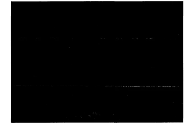
Our system relies on a A;d-tree for distributing and balancing the data. The spatial partitioning is done once initially and can be adaptively refined by the rendering times from previous frames. The initial tree only considers the number of bricks available in the data set, and attempts to evenly distribute them among processes, to the extent that is possible. When using static load balancing, this decomposition is determined and invariant for the life of the parallel job. Figure 2-2 depicts a possible configuration determined by the partitioner, and shows the corresponding fcd-tree.
Figure 2-2: Decomposition and corresponding fcd-tree for an 8x3x8 grid of bricks divided among 4 processors. Adjacent bricks are kept together for efficient rendering and com-positing. A composite order is derived dynamically from the camera location in relation to splitting planes. Note that the number of leaves in the tree is equal to the number of processes in the parallel rendering job.
When the dynamic load balancer is enabled, we use the last rendering time on each process to determine the next configuration. In our initial implementation, the metric we utilized was the total pipeline execution time to complete a frame. This included the time to read data from the disk, as well as compositing time, among other inputs. However, we found that I / O would dwarf the actual rendering time. Further, compositing time is
not dependent on the distribution of bricks. This therefore proved to be a poor metric. Switching the balancer to use the total render time for all bricks on that process gave significantly better results.
In order to compare different implementations, we implemented multiple load balancing algorithms, notably those described in Marchesin et al. [20] and Miiller et al.'s work [24]. In both cases, leaf nodes represent processes, and each process has some number of bricks assigned to it. In the Marchesin-based approach, we start at the parents of the leaf nodes and work our way up the tree, searching for imbalance among siblings. If two siblings are found to be imbalanced, a single layer of bricks is moved along the splitting plane. This process continues up to the root of the tree, at which time the virtual results are committed and the new tree dictates the resulting data distribution. In the Muller-based approach, we begin with the root node and use preorder traversal to find imbalance among siblings. Once imbalance is found, the process stops for the current frame. Instead of blindly shifting a layer of blocks between the siblings, the method derives the average rendering cost associated with a layer of bricks along the split plane, and shifts this layer if the new configuration would improve rendering times.
In addition to achieving a relatively even balance among the data, the fcd-tree is used in the final stages to derive a valid sort-last compositing order.
2.3 Rendering
Rendering is performed in parallel on all nodes using Tuvok, a volume rendering library which uses GLSL shaders to accelerate rendering on the GPUs.
2.3.1 Tuvok
Tuvok1 is a drop-in volume rendering library for handling extremely large data [30]. One of
the primary design goals of Tuvok is that it should be able to visualize data sets of incredible
Figure 2-3: Various render modes applied to the C60 dataset. In the top row ID and 2D transfer functions, isosurface extraction, and Clear View are shown. The bottom row shows the same views in anaglyph stereo mode. On the right is two by two mode featuring a 3D view, a MIP view (top right), and two slice views (bottom).
size on almost any commodity system. Through the work presented in this thesis, we have verified the correctness of the renderer with data sizes greater than 2 terabytes. This is achieved using a streaming, progressive rendering system guaranteeing interactive frame rates with adaptive quality. The generation of full quality imagery is also guaranteed on all configurations, with any data set, but may not happen interactively.
To achieve compatability across a large set of graphics processing units, Tuvok contains a variety of extra code paths for compatibility settings, which addresses a number of issues discovered in various OpenGL drivers. Tuvok contains multiple Tenderers, based on ray casting, 3D slicing, and 2D slicing, which span a large range of quality versus portability across GPUs and drivers. The wide variety of renderer types has been critical in supporting a large set of collaborators, as less technical users tend to have integrated graphics chips which lack support for even 3D textures. Another feature driven by this requirement is the ability to select the bit width of the framebuffer object (FBO) used for rendering, because we found that some drivers would switch to a software path when rendering into a 32-bit FBO.
Tu-Figure 2-4: Large data sets rendered with the Tuvok framework. The Visible human CT scan (a), the Wholebody data set (b) and the Richtmyer-Meshk ov instability RMI (c).
vok's compatibility and scalability. 'Air' represents a typical MacBook Air in 2010, using
a GeForce 9400M with little available RAM. 'Pro' represents a MacBook Pro, which has about half the memory required to load up the full Richtmyer-Meshkov instability, and uti-lizes a more powerful GeForce 9600. 'Vista' is a high-end workstation with enough memory to fit all data sets in-core, and a powerful NVIDIA Quadro 5800. The data span a range of sizes and complexities; 'C60' is a small, test data set; the visible human male CT scan is still relatively small, but useful for comparisons due to its popularity; the 'wholebody' data set is slightly larger and heavily anisotropic; the RM ('Richtmyer-Meshkov') Instability is a large data set by desktop metrics.
For these timings the progressive rendering has been disabled: only the time to render the maximum quality image for the given view was measured. With the progressive ren-dering turned on all data sets render at the chosen refresh rates on all systems. Note that the systems used in the test cover chipset integrated GPUs as well as also high end PC configurations. Timings are presented for small data sets as well as reasonably sized CT scans and simulations.
2.3.2 Visit Integration
We have developed and integrated the Tuvok library into Visit to perform extremely large scale volume renderings. Our work utilizes the 3D slicing volume renderer, which provides a good balance between performance and compatibility. For nodes without access to a GPU,
data set C60 Molecule 128 X28 128 Bbtt = 2 MB See Figure 2-3 V H Male C T 512 512 1884 Sbit = 471 MB
See Figure 2-4a
"Wholebody 512 512 3172 16bit = 1586 M B See Figure 2-4b RM Instability 2048 2048 1920 &btt = 7680 MB See Figure 2-4c Air 110/184 380/500 680/700 5523/6112 P r o 80/124 526/744 587/984 3112/3520 Vista 12/14 48/76 126/301 196/321
Table 2.1: Tuvok timings in milliseconds for various data sets and configurations. "Air": MacBook Air, 2GB RAM, Onboard Geforce 9400, "Pro": MacBook Pro, 4GB RAM, Geforce 9600, "Vista": PC running Windows Vista, 24GB RAM, NVIDIA Quadro 5800. All tests were performed in isosurface-mode (first value) and in ID transfer function mode (second value), using the ray casting renderer sampling twice per voxel, into a 1024 • 1024 viewport. The camera was zoomed such that the data set covered the entire viewport, and the data were divided into bricks of size 2563.
data are rendered through the Mesa library's 'swrast' module, which executes vertex and fragment shaders on the CPU [25]2.
Since Visit lacks robust support for multiresolution data, the progressive rendering features of Tuvok were not utilized. Instead, Visit's I/O routines were unmodified, and we utilized Tuvok's external data set API to feed data from Visit to the renderer. Tuvok could still improve performance and render data progressively by reducing screen resolution and sampling rate, however we chose to disable this feature as it simplifies the presentation of performance data. Tuvok is simply given a set of bricks and asked to render them. Each process in the MPI job does this independently, and does not take into account the screen space projection of the data.
Data are forwarded "as-is" from disk, without modification or transformation to its type. In our experiments, this means that floating point data flows all the way through the
2As one might guess, performance in this configuration is poor. We do not formally give performance information for this configuration, but informally: we found a NVIDIA GTX 8800 to be about 500 times faster than using Mesa's 'swrast' renderer.
pipeline, and becomes the input to the Tenderers - we push the native-precision data down to the GPU and render it at full resolution. Of course, data are effectively quantized due to the limited resolution of a transfer function.
We find this architecture compelling because it removes any need to pre-process the data. Visit's parallel pipeline execution is based wholly around the bricks given as input to the tool. Our main restriction is the size of each individual brick: since we utilize an out-of-core volume renderer, we can stream sets of bricks through a GPU, even if the stream exceeds the maximum 3D texture size or GPU memory available. However, each individual brick must be small enough to fit within the texture memory available on a GPU.
In practice, this limitation has not affected how we generated or visualized the data for this work. Should the need arise, we could re-brick the data set to sizes more amenable for visualization.
2.4 Compositing
After rendering completes, each node has a full image with a subset of the total data volume rendered into it. A compositing step takes these partial images and combines them to produce the final result. Although we did not expect compositing to be a significant factor in the performance of the overall system, we nonetheless incorporated a well-studied compositor instead of implementing one ourselves. We chose the IceT parallel compositing library [23], for its ease of integration and proven results. In external work, we have observed the IceT compositor to be up to 8 times faster than the traditional Visit compositing code path. We extended the compositing subsystem to derive an order from the fcd-tree for the data passed on to IceT.
IceT implements a number of different compositing modes. However, not all of them support what IceT calls ordered compositing, as is needed for object-parallel distributed volume rendering. For this work, we have utilized the so-called reduce strategy, which, since we only configure a single 'tile' in our system, essentially simplifies [23] to an implementation
CHAPTER 3
EVALUATION
We implemented and tested our system on Lens, a GPU-accelerated visualization cluster housed at ORNL. However, we were only able to access 16 GPUs on that machine. In order to access a larger number of GPUs, we transitioned to Longhorn, a larger cluster housed at the Texas Advanced Computing Cluster. Specifications for each cluster are listed in Table 3.1. Due to machine availability and configuration, we were not able to fully utilize either machine.
3.1 Rendering Times
The two dominant factors in distributed memory visualization performance are the time taken to render the data and the time taken to composite the resulting sub-images. These have the largest impact on usability, because they comprise the majority of the latency a user experiences: the time between when the user interacts with the data and when the results of that interaction are displayed.
Our data originated from a simulation performed by the Center for Simulation of Ac-cidental Fires and Explosions (C-SAFE), designed to study the instabilities in a burning helium flame. In order to study performance at varying resolutions, we resampled this data to 10243, 20483, 40963, and 81923, at a variety of brick sizes. We then performed tests,
varying data resolution, image resolution, choice of brick size, and number of GPUs, up to 256. Unless noted otherwise, we divided the data into a grid of 8x8x8 bricks for parallel processing (larger data sets used larger bricks), and rendered into a 1024x768 viewport.
C o m p o n e n t
Number of nodes GPUs per node Cores per node Graphics card Per-node Memory Processors Interconnect Lens 32 2 16 NVIDIA 8800 GTX 64 GB 2.3 GHz Opterons DDR Infiniband Longhorn 256 2 8 NVIDIA FX 5800 48 GB 2.53 GHz Nehalems Mellanox QDR InfiniBand Table 3.1: Configuration of GPU clusters utilized.
Figure 3-1 shows the scalability on the Longhorn cluster. The principal input which affects rendering time is the data set size, as one might expect. These runs were all done using 2 GPUs per node, except the "64 GPUs, 1 GPU/node" case, which was run on 64 nodes, each accessing a single GPU. With very large data, there is a modest increase in performance for this experimental setup.
As can be seen in Figure 3-2, the brick size, generally, has little impact on performance. A parallel volume Tenderer's performance is dictated by the slowest component though, and therefore the average rendering time is less important than the maximum rendering time. Taking that into account, it is clear that brick sizes that are not a power of two are poor choices. Dropping down to 1283, we can see that per-brick overhead begins to become more
noticeable, impacting overall rendering times. We found larger brick sizes of 5123 get the
absolute best performance, with 2563 a good choice as well, as the differences are minor
enough that they may be considered sampling error. Of course, such recommendations may be specific to the GPUs used in Longhorn.
We were initially surprised to find that the image resolution, while relevant, was not a significant factor in the overall rendering time. When developing single GPU applications that run on a user's desktop, our experience was the opposite: that image size did play
25 20 -a c o o CD 0) 15 -64 GPUs, 1 GPUs/node —<-64 GPUs, 2 GPUs/node --•*-• 128 GPUs, 2 GPUs/node ---*-256 GPUs, 2 GPUs/node a 1024° 2048 4096°
Dataset Size (voxels)
8192°
Figure 3-1: Overall rendering time when rendering to a 1024x768 viewport on Longhorn. This incorporates both rendering and compositing, and therefore shows the delay a user would experience if they used the system on a local network. Data points are the average across many frames. For these results we used a domain consisting of 133 bricks (varying
brick size), with the exceptions that all runs in the 128 GPU cases used 83 bricks, and the
run for the 81923 data set was done using 323 bricks.
a significant role in performance. We first thought this was due to skipping bricks which were 'empty' under our transfer function - our domain is perfectly cubic, yet as is displayed in Figure 2-1, very little of the domain is actually visible - but even after changing to a transfer function with no "0" values in the opacity map, rendering times changed very little. We concluded that the data sizes are so large compared to the number of pixels rendered that the image size is not relevant as a factor.
11 10 9 8 # 6 -CO T3 (1) 3 DC 4 3 2 --) I i i i i i i I 128 256 315342 373 512
Brick Size (voxels, cubed)
Figure 3-2: Rendering time as a function of brick size. Range bars indicate the minimum and maximum times recorded, across all nodes, for that particular brick size; high disparity indicates the rendering time per-brick was highly variable, and load imbalance was therefore likely. All tests were done with a 40963 data set statically load balanced across 128 GPUs
on 64 nodes, using a scripted camera which requested the same viewpoints each run. Note that the choice of brick size matters little in the average case, but bricks using non-power-of-two sizes give widely varying performance. Brick sizes of 5123 technically give the best
performance, though raw data show it is only hundredths of a second faster than bricks which had 2563 data points.
3.2 Memory Strain
In our initial implementation on Lens, we noticed that we began to strain the memory allocators while rendering a 30003 data set, as we approached low memory conditions. Our
volume renderer automatically accounts for low memory conditions and attempts to free unused bricks before failing outright. However, an operating system will thrash excessively before finally deciding to fail an allocation, and therefore during the time leading up to a failed allocation, performance will drop considerably. Worse, we are working in a large
1 I 0.38 \! * 0.36 I ' ' ' ' ' ' 0 10 20 30 40 50 60 70
Frame
Figure 3-3: Rendering times, per frame, for the in-core and out-of-core approaches to ren-dering a 10243 data set (which fits comfortably in memory) across 16 GPUs. Additional
processing in the out-of-core case does not negatively impact performance.
existing code base, and attempting to manage allocations outside our own subsystem would prove unwieldy. As such, we found the original scheme to be unstable; the rendering system would create memory pressure, causing other subsystems to fail an allocation in areas where it may be difficult or impossible to ask our volume renderer to free up memory.
To solve this problem, we render the data in a true out-of-core fashion: bricks are given to the renderer, rendered into a framebuffer object, and immediately thrown away. We might expect that out-of-core algorithms would have more per-block overhead and therefore be slower than an in-core algorithm. As shown in Figure 3-3, the out-of-core approach actually out-performs the analogous in-core approach even when there is sufficient memory to hold the data set. In this case, finding which texture to delete in a data structure took logarithmic lookup time in the in-core approach, whereas the conservative approach taken in the
out-D a t a s e t Size 10243 20483 40963 81923 Rendering (s) 0.06141 0.35107 2.50984 19.60648 Readback (s) 0.00328 0.00377 0.00377 0.00373 C o m p o s i t i n g (s) 0.06141 0.07673 0.29533 0.51799 Total (s) 0.12610 0.43157 2.80894 20.12820 Table 3.2: Breakdown of the different pipeline stages for various data set sizes, when running on 256 GPUs and rendering into a 1024x768 viewport. All times are in seconds. The 10243, 20483, and 40963 case used 133 bricks (varying brick size); the 81923 case used 323
bricks, making each brick 2563. Compositing time rises only artificially; if a node finishes
rendering before other nodes, the time it must wait was included under 'Compositing' due to an artifact of our sampling code. Thus, the data imply that larger data sets see more load imbalance.
of-core algorithm meant the container maxed out at one element, which accounted for the very minor improvement to performance.
3.3 Readback and Compositing
In earlier results, particularly with GPU-based rendering architectures, the community was generally concerned with the time required to read the resulting image data from the GPU into the host's memory [19]. Our study did not provide corroboration of this concern, which we interpret as a positive data point with respect to evolving graphics subsystems. Our system did demonstrate that this time increased as the resolution grew, but as can be seen in Table 3.2, even at 1024x768 this step took only thousandths of a second.
As expected, the time required for image composition is significantly reduced when tak-ing advantage of the GPUs available in a visualization cluster. Since a GPU can render much faster than a software-based renderer, one can achieve acceptable rendering perfor-mance using far fewer nodes. Furthermore, because compositing scales linearly with the number of nodes involved in the compositing process, compositing performance improves significantly when utilizing fewer nodes.
3.4 Load Balancing
We also sought to examine the utility of load balancing algorithms for our system. We have implemented the algorithms as presented in two recent parallel volume rendering papers [20, 24], and compared rendering times to each other and to a statically balanced case. Figure 3-4 illustrates the comparisons, where the times shown are the maximum of all processes.
We did a variety of experiments with multiple load balancer implementations, using 8 or 16 GPUs. Our initial fly-through sequence proved to be inappropriate for the application of a load balancer, as there was not enough imbalance in the system to observe a significant benefit. We then attempted to zoom out of the dataset, but this resulted in rendering times that increased on all nodes; it was not a case the balancers we implemented could effectively deal with. We found many cases where the balancers would shift data to a node that was previously idle or at least doing very little work, and a frame or two later the workload on such nodes would spike. This occurred because these nodes had both 1) received new data as part of the balance and, 2) retained old data as part of the initial decomposition or older balancing processes. The sudden additional workload of previously invisible bricks caused these nodes to over compensate, sending data to other "idle" nodes - nodes which would experience the same problem a frame or two later.
In previous work, authors have praised the effect load balancing has when zooming in to a data set [9,20]. Zooming naturally creates imbalance, as some nodes end up with data which are not rendered under the current camera configuration, and therefore the node has no work to do.
3.4.1 Algorithm Details
We recreated previous load balancing implementations ( [20,24]) as faithfully as possible, and found that zooming in to the data set was a task that was well-suited for load balancing. Still, we encountered issues even with this case. For the algorithm given in [20], we observed that data would move back and forth between nodes quite frequently, having a negative
Time Spent Rendering
15 20
Frame number
Figure 3-4: The maximum rendering time across all nodes under various balancing algo-rithms. The numbers after some algorithms indicate thresholds: rendering disparity under these thresholds is ignored.
impact on overall rendering time. We therefore introduced a 'threshold' parameter to the existing algorithm, in an attempt to limit this 'ping-pong' behavior. As we move up the tree, imbalance between the left and right subtrees is subject to this threshold; if it does not exceed the threshold, the imbalance is ignored. This is a very useful parameter for ensuring that we do not move data too eagerly. Generally, setting this threshold too high yields behavior equivalent to the static case; setting it too low leads to a considerable amount of unnecessary data shifting. We found that in many cases data shifting overcompensated for minor, expected variations (such as those one might expect from differing brick sizes; see Figure 3-2). For example, Figure 3-4 shows that low thresholds display an obvious 'ping-pong' effect as nodes overcompensate for increased rendering load.
Miiller et al. describe a different balancing system [24]. This system calculates the average cost of rendering a brick, and therefore has a clearer idea of what the effect of moving a given set of bricks will have on overall system performance. Further, they introduce additional parameters which add some hysteresis to the system. This parameter can help reduce the 'ping-pong' effect of nodes sending data to a neighbor, only to receive in the next frame when the neighbor becomes overloaded.
3.4.2 Results
We found that this algorithm did do intelligent balancing for reasonable settings of these parameters, and the additional parameters could be successfully used to reduce excess data reorganization. Still, we found two issues with the approach: for one, the assumption that 'all bricks are equal' did not pan out for our work. Even assuming uniform bricks for a data set (true for our case, but likely not in a general system), one can see in Figure 3-2 that the time to render a brick sees variation on the order of a second. Secondly, despite experimenting with parameter settings, we found it difficult to get the algorithm to choose the 'best' set of nodes for balancing. In many cases, we found a particular node was an outlier, consistently taking the most time to render per frame. Yet it was common for this algorithm to balance different nodes. While rendering times would generally improve,
W -o c o o © o E _c CD TJ c
o
rr
1.6 1.4 1.2 1 0.8 0.6 0.4 0.2 1 -i I S - * ' I T * i i i i i Process 0 Process 1 Process 2 I Process 3 _i- . Process 4 s\? A. Process 5 \>\ -. a •* Process 6 \fe-. ^ Process 7 ; •• Y •• * *'« GJ\ "• \ - A . * ^ s-s.^V ®'S'"B-«~B..B. * i L — 1 is n ...x— • • * -B . .«.. . A -0 5 1-0 15 2-0 25 3-0 35Frame
Figure 3-5: Per-process rendering times for the 'Miiller' line given in Figure 3-4. the system's performance is determined by the slowest node, and therefore making the fast nodes faster does not help overall performance.
This was apparent in the tests described in 3-4: the algorithm quite clearly balanced between some of the nodes, but the slowest node was never balanced, and therefore the user-visible performance for this run was equivalent to the static case. Figure 3-5 shows a more detailed analysis of the execution of the Miiller algorithm that generated the data for Figure 3-4. The per-node rendering times in Figure 3-5 show that process 7 is usually the last process to finish and is often much slower than the next to the last. As evident from the lack of sudden discontinuities in that process' rendering times, however, no bricks from process 7 move to other nodes. Therefore rendering times decrease but the maximum rendering time does not change.
would yield fruitful results. Furthermore, the algorithm explicitly attempts to avoid visiting the entire tree, as an attempt to bound the maximum time needed to determine a new balancing. In our work, we did not observe cases where iterating through nodes in the tree had a measurable impact on performance, and feel that by doing so the algorithm could obtain the global knowledge it needs to balance data effectively. Both of these extensions are left to future work.
3.5 Observations
In Chapter 1, we noted a variety of questions which the design of our system allows us to address.
• Rendering vs. Compositing. As shown in Table 3.2, sub-second rendering times are achieved using a very small number of nodes, relative to previous work. This relieves a significant source of work for compositing algorithms.
• Overhead of GPU Transfer. Table 3.2 shows readback time to be on the order of thousandths of a second for common image sizes. Measuring texture upload rates is difficult with the asynchronous nature of current drivers and OpenGL, but we did not find evidence to suggest this was a bottleneck.
• Importance of Load Balancing. A dynamic load balancer can have a very worthwhile impact on performance. However, it can also lower the performance of the system. Load balancers generally come with some number of tunable parameters, and useful settings for these parameters are difficult to determine a priori, and likely impossible for an end-user to effectively set. We observed that dynamic load balancing for volume rendering struggled in some of the cases often encountered in real world environments and, for this reason, believe there is still a gap between state of the art and production-quality systems. We see a great opportunity for future work in this area.
data sizes - up to 81923 voxels - is possible on relatively few nodes. Further, data
CHAPTER 4
SUMMARY
This thesis has presented a system for volume rendering massive data on large scale GPU-enabled clusters. The system scales effectively up to data sets of 81923 (2.1 terabytes on
disk) and results imply that the system could take advantage of many more GPUs before compositing time begins to dominate rendering time.
With this study, we demonstrated that GPU accelerated rendering provides compelling performance for large scale data sets. Figure 3-1 demonstrates our system rendering data sets which are among some of the largest published thus far, using far fewer nodes than pre-vious work. This work shows that a multi-GPU node is a great foundational 'building block' to compose larger systems capable of rendering very large data. As the performance-price ratio of a GPU is higher (provided it can effectively parallelize the workload) than CPU-based solutions, this work makes the case for spending more visualization supercomputing capital on hardware acceleration, and acquiring smaller yet more performant clusters.
Reports on the time taken for various pipeline stages demonstrate that PCI-E bus speeds are fast enough that readback performance is not as great a concern as it was a few years ago. However, it remains to be seen if contention will become an issue if individual nodes are made 'fatter', utilizing additional GPUs. The 1 versus 2 GPU per node results given in Figure 3-1 suggest that multiple GPUs do contend for resources, but at this scale the differences are not yet significant enough to warrant moving away from the more cost-effective 'fat' node architecture. Given the relatively few nodes needed for good performance on large data, as well as external work which has successfully scaled compositing out to tens of thousands of cores, scaling compositing workloads out to tens of thousands of cores, it
seems likely that the relatively 'thin' 2-GPU-per-system architecture can be made to scale to much larger systems than the ones utilized for this work.
4.1 Future Work
We would like to study our system with higher image resolutions, such as those available on a display wall, and larger numbers of GPUs. At some point, we expect compositing to become a significant factor in the amount of time needed to volume render large data, but we have not approached the cross-over point in this work, due to the use of 'desktop' image resolutions and low numbers of cores.
Our system allows substituting a Mesa-based software renderer when a GPU is not available. This provided a convenient means of implementation within an existing large software system, in particular because it allows pipeline execution to proceed unmodified through the rendering and compositing stages. However, tests very quickly showed that it is not viable to use software Tenderers when a GPU is available, and usually ended up hurting performance more than helping. Therefore, we advocate trading access to more cores for the guarantee that we will obtain GPUs for each core we do get.
An alternate system architecture would be to decouple the rendering process from the other work involved in visualization and analysis, such as data I/O, processing, and other pipeline execution steps. In this architecture, all nodes would read and process data, but processed, visualizable data would be forwarded to a subset of nodes for rendering and compositing. The advantage gained is the ability to tailor the available parallelism to the visualization tasks of data processing and rendering, which, as we have found, can benefit from vastly different parallel decompositions. The disadvantages are the overhead of data redistribution, and the wasted resources that arise from allowing non-GPU processes to sit idle while rendering.
Our compositing algorithm assumes that the images from individual processors can be ordered in a back-to-front fashion to generate the correct image. For this thesis, we met
this requirement by using regular grids, which are easy to load balance in this manner. It should be possible to also handle certain types of curvilinear grids and a subset of nested AMR grids. Extensions to handle unstructured grids would be difficult, but represent an interesting future direction.
Load balancing is an extremely difficult problem, and we have barely scratched the surface here. The principal difficulty in load balancing is identifying good parameters to control how often and to what extent the balancing occurs. We would like to see ideas and algorithms which move in the direction of user-friendliness: determining the most relevant parameters and deriving appropriate values for them automatically.
Appendix A
PARALLEL A P P R O X I M A T E
I M A G E C O M P O S I T I O N
A . l Parallel Compositing Overview
Parallel image compositing scales primarily with the image resolution and the number of processes which take part in the compositing process. The resolution determines the amount of work done for every image, though with modern CPUs at typical "desktop" resolutions, the Porter and Duff Over operator [28] can be applied so quickly as to make this factor irrelevant [10]. If we ignore the case of high-resolution display walls, then, the primary contributing factor to the time taken for a parallel image compositing algorithm is the number of processes. More processes implies more communication, the bane of any parallel algorithm.
Parallel volume rendering of large data is a challenging problem. Methods for decom-posing the workload are well-studied [10,15,20,24], yet no clear approach has been identified which can provide a consistently positive impact on rendering performance. Furthermore, load imbalance increases naturally as a function of data set size. To make matters worse, the choice of sizes for subdomains in large simulations is not made with the consideration that these subdomains will be mapped directly into the 3D texture memory of a GPU. Improper choice of texture sizes (in particular non-power-of-two texture sizes) can cause severely variable rendering performance - even if subdomains are all the same size [10].
For more complex data types, such as adaptive mesh refinement data [1], the variable workload problem becomes even worse. Therefore it is highly desirable to utilize com-positing algorithms which can begin to make progress prior to completion of the rendering process across all nodes. Yet many popular algorithms, such as binary swap [18], will stall until a "neighbor" process completes the rendering workload. The ability to perform large subsets of the image composition process will allow a system to mitigate the effects of se-vere rendering imbalance between nodes. Compositing algorithms which fit this mold are generally of the 'direct send' [12] type. Unfortunately direct send's scalability is limited with large numbers of processors, due to an all-to-all communication pattern.
In this chapter we outline the beginnings of a new algorithm which is based around two core observations:
• For parallelization purposes, it is highly desirable for a computation to be commuta-tive.
• When compositing a set of n semi-transparent images, it is extremely likely that a proper subset of n will dominate the computation.
The end goal is to develop an algorithm which lacks a barrier between the rendering and compositing stages. Such an algorithm could not be developed within the constraints of this thesis, but we feel it is important to document our progress to this point regardless.
A.2 Expansion of the Over Operator
Porter and Duff's over operator [28] forms the basis of image composition, and therefore distributed volume rendering. The operator is defined as:
A over B = CAO-A + (1 - C\A)CBOI-B (A.l) If we extend that operator to 3 images, the weighting by 1 — a A applies to both images
CAaA + (1 - aA){CBaB + (1 - aB){Ccac)) (A.2)
If we then expand that expression by distributing all terms, we obtain:
CAOLA + CBOCB + Ccac
-asCcotc — O-ACBO-B
+aAaBCcac (A.3)
To generalize, for N images, 1 being the topmost image and n being the bottom image, we'll get an expression that looks like:
»=i n t,J=l,2 n j,j,fc=l,2,3 n - 2_j ctta-,akaiCi t,j,k,l=l,2,3,4
On the surface, this form of the equation has a couple advantageous properties: 1. It is a sum of products instead of a product of sums. Such expressions are, in general,
easier to parallelize.
• In particular, there are no ordering requirements, implying that computation of the expression can begin as soon as any two processors have finished the rendering process.
3 2 1 0 -1 -2 -3 -4 CO c (0 > 1 2e+06 1e+06 800000 600000 400000 200000
Terms Increase Accuracy
-"!' 1 1 + 1 1 i 1 •* I + 1 ~-l - f l + i -+ l ^ 1 L I <r K 1 1 1 data smooth f n "-1 "-1 * 1 " -" 8 10 12 Maximum number of terms
Number of Terms 14 16 18 n r Values Required smoothed _ i i i i _ 6 8 10 12 14 Maximum number of terms
16
20
18 20
Figure A-1: Approximating image composition using a different number of E-terms. 2. Diminishing returns: the first few E-terms will dominate the value of the expression.
This suggests that we can ignore some of the later expressions' E-terms without having a noticeable impact on the final value of the expression.
Figure A-1 demonstrates these diminishing returns for a composition of 20 images. The top graph shows the error of the method as compared to the reference Porter & Duff-computed answer. The X-axis of Figure A-1 varies the number of E-terms which were used; at the x — 1 location, this gives the error of the expression J^?=i ^3aj a s compared to the
Porter and Duff calculation.
The bottom graph in Figure A-1 shows the number of "values" used in the sum (each element in a E-term counts as one 'value'; thus there are n values in the initial Y^=i ajCj
term). When we get halfway through the E-terms, the possible combinations of a's and C's begins to drop, causing the inflection point in the graph. Stated another way: the number
of terms in J^x is the number of ways we can choose x a's out of n (i.e. (^)), and therefore
when x > §, the number of choices begins to drop.
This is promising, because it shows that we don't need all of the E-terms to achieve a relevant result. Indeed, using ^ E-terms, we can achieve a result which is practically indistinguishable from the ground zero truth. Even with just 7 E-terms in the 20-image case, the result is close enough that it seems it would be a reasonable approximation.
A . 3 Significance of T e r m s
As demonstrated in Equation A.3, the Porter and Duff over operator can expand into a set of sums which multiply a set of alpha values with a single color. The number of terms involved in each successive Riemann sum shrinks as we choose more alphas out of the available set of n. For example, when n is 5, the total number of terms added is (j) + (2) + (3) + (4) + (5).
We can take advantage of a series of numeric and color properties to remove a large number of these terms. First we assume that am £ [0 : 1), where am represents the
maximum opacity observed across the set of all images. Strictly speaking, am could be 1,
but this case is unlikely in practice and it suffices to special case that event.
Given that any term in the fc'th Riemann sum will involve (£) alphas, the maximum value which any term can contribute is a ^ . Further, am < 1 =>• a ^ < am, or additional
alphas will push the resultant calculation closer to 0.
The context in which any calculation is carried out can be critical to understanding edge cases. This computation will be performed using floating point numbers in the best case, and of course floating point representations do not have arbitrary precision on any real computer. If we have 3 digits of precision, than any expression smaller than 0.001 would not effect the computation: it would evaluate to 0, since it cannot be stored, and is therefore irrelevant. Let us call the number of digits of precision L.
It is therefore safe to say that any of the terms within the Riemann sums in the expanded compositing equation (e.g. Equation A.3) which would evaluate to < L would not have any
result in the final image, as the value could not be represented and would be stored as 0. We emphasize that we have not demonstrated that the addition of such terms will have no
discernible effect, but rather that the addition of such terms will have no effect.
Stated explicitly, this means that each term must exceed L to be relevant to the over operator computation. In the k'th Riemann sum, each term will involve k alphas. The largest each term could thus be is o^C^, but since we assume Ck G [0 : 1), we can drop C^ and still consider a ^ to be an upper bound.
c<m< L ^> irrelevant (A.4)
Note that this result does not depend on n, the number of images in the computation. This is because we are proving that each term in a Riemann sum is going to be represented as zero; if each term is zero, then their summation must of course also be zero.
k = \\ogaJL)] (A.5)
It turns out L is given in the C header f l o a t . h and is defined to be 1.19209e — 7 for IEEE-754 floating point. Given a maximum alpha of 0.5, for example, this means that
k — \logo,5(1.19209 x 10~7)] =>• k = 24. The interpretation is that no term with more than
24 alpha values in it will be non-zero. Thus all terms with more than 24 alphas can be discarded a priori.
In this thesis, we studied volume rendering which utilized up to 256 images. The total number of terms in this compositing case is Sfi^( ^6), however only E?:l1(2^6) will be
relevant when the maximum alpha is 0.5; put another way, 3.19947522472 x 10~42 percent
of the values affect the computation. Other work suggests that as many as 36,000 cores may be relevant for volume rendering large data, when GPUs are not available [11]. With 36,000 cores comes 36,000 images, yet still only E2^ (3 6f0 0) terms will be relevant.
A.3.1 Application
The problem facing the aforementioned method of calculating a composited image is how to utilize the new framework effectively. As an example, choose an arbitrary term in the expansion, such as aoasa4a5ai2Ct2oC2o, and note how many different images must be rep-resented. To compute this value, we need to get the alpha channels from images 0, 3, 4, 5, 12, and 20, as well as the color channel[s] from image 20, together.
There are a couple ways this could be done. One method is to colocate some subset of the terms together in one process, and others in another, multiply the subsets together, and then finally send the subset to one process or the other to multiply both subsets together with the color. Another method is to say that we need all of the associated alphas in the above term to be colocated with the 20"1 color, and simply send all of the necessary alpha
values to whatever process has the 20*^ color.
This second option does not have sufficient advantages to be worthwhile. This method boils down to direct send, with a unique way of computing the final color. The network traffic will be substantial and incredibly bursty, as most nodes finish around the same time and send large numbers of alpha values to a process predetermined by screen-space subdivision.
The first option negates the asynchronous benefit we were searching for. Note that we could apply this operation hierarchically: processes 0 and 3 could calculate ao«3 whilst pro-cesses 4 and 5 calculate 0405. Then one process in each of those groups could communicate to calculate aoa3a4as. Regardless of whether or not one takes advantage of this hierarchi-cally, we are still imposing staged calculations, or implicit barriers, into our compositing algorithm. If process 3 takes longer to generate an image than other processes, then the computation stalls.
BIBLIOGRAPHY
[1] M.J. Berger and J. Oliger. Adaptive Mesh Refinement for Hyperbolic Partial Differ-ential Equations. J. of Comput. Phys., 53, 1984.
[2] Brian Cabral, Nancy Cam, and Jim Foran. Accelerated volume rendering and tomo-graphic reconstruction using texture mapping hardware. In VVS '94: Proceedings of
the 1994 symposium on Volume visualization, pages 91-98, New York, NY, USA, 1994.
ACM. h t t p : / / d o i . acm. org/10.1145/197938.197972.
[3] Hank Childs, Sean Ahem, Kathleen Bonnell, David Bremer, Eric Brugger, David Camp, Rich Cook, Marc Durant, Thomas Fogal, Cyrus Harrison, Randy Hudson, Harinarayan Krishna, Jeremy Meredith, Mark Miller, Paul Navratil, Dave Pugmire, Oliver Ruebel, Allen Sanderson, Josh Stratton, Dave Semeraro, Gunther Weber, and Brad Whitlock. Visit Visualization and Analysis Software Package, h t t p : / / v i s i t . l l n l . g o v / , 2001-2011.
[4] Hank Childs, Eric Brugger, Kathleen Bonnell, Jeremy Meredith, Mark Miller, Brad Whitlock, and Nelson Max. A Contract Based System For Large Data Visualization. In Proceedings of IEEE Visualization 2005, 2005. h t t p : / / w w w . i d a v . u c d a v i s . e d u / func/return_pdf?pub_id=890.
[5] Hank Childs, Mark Duchaineau, and Kwan-Liu Ma. A scalable, hybrid scheme for volume rendering massive data sets. In Proceedings of Eurographics Symposium on
Parallel Graphics and Visualization, pages 153-162, May 2006. h t t p : / / w w w . i d a v .
[6] Timothy J. Cullip and Ulrich Neumann. Accelerating volume reconstruction with 3d texture hardware. Technical Report TR93-027, University of North Carolina at Chapel Hill, 1994. h t t p : / / g r a p h i c s . u s e . e d u / c g i t / p d f / p a p e r s / V o l u m e _ t e x t u r e s _ 9 3 . p d f . [7] Robert A. Drebin, Loren Carpenter, and Pat Hanrahan. Volume Rendering. In
SIGGRAPH '88: Proceedings of the 15th annual conference on Computer graphics and interactive techniques, pages 65-74, New York, NY, USA, 1988. ACM. h t t p :
/ / d o i . a c m . o r g / 1 0 . 1 1 4 5 / 5 4 8 5 2 . 3 7 8 4 8 4 .
[8] Stefan Eilemann and Renato Pajarola. Direct Send Compositing for Parallel Sort-Last Rendering. In Proceedings of the Eurographics Symposium on Parallel Graphics and
Visualization, pages 29-36, 2007. h t t p : / / d o i . a c m . o r g / 1 0 . 1 1 4 5 / 1 5 0 8 0 4 4 . 1 5 0 8 0 8 3 .
[9] Faith Erol, Stefan Eilemann, and Renato Pajarola. Cross-segment load balancing in parallel rendering. In Torsten Kuhlen, Renato Pajarola, and Kun Zhou, editors,
Pro-ceedings of the 11th Eurographics Symposium on Parallel Graphics and Visualization,
pages 41-50, April 2011. h t t p : / / v m m l . i f i . u z h . c h / f i l e s / p d f / p u b l i c a t i o n s / C S L B . pdf.
[10] Thomas Fogal, Hank Childs, Siddharth Shankar, J. Kriiger, R. D. Bergeron, and P. Hatcher. Large Data Visualization on Distributed Memory Multi-GPU Clusters. In Proceedings of High Performance Graphics 2010, pages 57-66, June 2010.
[11] Mark Howison, E. Wes Bethel, and Hank Childs. MPI-hybrid Parallelism for Vol-ume Rendering on Large, Multi-core Systems. In Eurographics Symposium on Parallel
Graphics and Visualization (EGPGV), Norrkoping, Sweden, May 2010. LBNL-3297E.
[12] William M. Hsu. Segmented Ray Casting for Data Parallel Volume Rendering. In PRS
'93: Proceedings of the 1993 Symposium on Parallel Rendering, pages 7-14, New York,
[13] Greg Humphreys, Mike Houston, Ren Ng, Randall Frank, Sean Ahem, Peter D. Kirch-ner, and James T. Klosowski. Chromium: A Stream-Processing Framework for In-teractive Rendering on Clusters. In SIGGRAPH '02: Proceedings of the 29th annual
conference on Computer graphics and interactive techniques, pages 693-702, New York,
NY, USA, 2002. ACM Press, h t t p : / / c i t e s e e r x . i s t . p s u . e d u / v i e w d o c / s u m m a r y ? d o i = 1 0 . 1 . 1 . 1 9 . 7 8 6 9 .
[14] Jens Kriiger and Riidiger Westermann. Acceleration Techniques for GPU-based Volume Rendering. In Proceedings IEEE Visualization 2003, 2003. h t t p : / / w w w c g . i n . t u m . d e / R e s e a r c h / d a t a / v i s 0 3 - r c . p d f .
[15] Won-Jong Lee, Vason P. Srini, and Tack-Don Han. Adaptive and Scalable Load Bal-ancing Scheme for Sort-Last Parallel Volume Rendering on GPU Clusters. 2005. [16] Marc Levoy. Efficient Ray Tracing of Volume Data. A CM Trans. Graph., 9(3):245-261,
1990. h t t p : / / d o i . a c m . o r g / 1 0 . 1 1 4 5 / 7 8 9 6 4 . 7 8 9 6 5 .
[17] Kwan Liu Ma, James S. Painter, Charles D. Hansen, and Michael F. Krogh. A Data Distributed, Parallel Algorithm for Ray-Traced Volume Rendering. In PRS '93:
Pro-ceedings of the 1993 symposium on Parallel Rendering, pages 15-22, New York, NY,
USA, 1993. ACM. h t t p : / / d o i . a c m . o r g / 1 0 . 1 1 4 5 / 1 6 6 1 8 1 . 1 6 6 1 8 3 .
[18] Kwan-Liu Ma, James S. Painter, Charles D. Hansen, and Michael F. Krogh. Parallel Volume Rendering Using Binary-Swap Compositing. IEEE Comput. Graph. Appl., 14(4):59-68,1994. h t t p : / / c i t e s e e r x . i s t . p s u . e d u / v i e w d o c / s u m m a r y ? d o i = 1 0 . 1 . 1 . 104.3283.
[19] S. Marchesin, C. Mongenet, and J.-M. Dischler. Multi-GPU Sort-Last Volume Visual-ization. In EG Symposium on Parallel Graphics and Visualization (EGPGV'08),
Euro-graphics, April 2008. h t t p : / / i c p s . u - s t r a s b g . f r / ~ m a r c h e s i n / e g p g v 0 8 - m u l t i g p u .