Modelling travel time in urban networks: comparable measures
for private car and public transport
Maria Salonen
a,⇑, Tuuli Toivonen
a,b aDepartment of Geosciences and Geography, University of Helsinki, P.O. Box 64 (Gustaf Hällströmin katu 2), 00014 Helsingin yliopisto, Finland b
Department of Biosciences, University of Helsinki, P.O. Box 56 (Viikinkaari 9), 00014 Helsingin yliopisto, Finland
a r t i c l e
i n f o
Keywords: Accessibility Car Door-to-door approach Public transport Travel mode Travel timea b s t r a c t
Analysing the accessibility disparity between different travel modes is recognised as an efficient way to assess the environmental and social sustainability of transport and land use arrangements. Travel times by different travel modes form an essential part of such an analysis. This paper aims to assess the com-parability of different methods for calculating travel time by different travel modes. First, we briefly review the methods used in previous studies and identify different typical approaches, which we then compare. We use three computational models respectively for car and public transport (PT), imple-mented in our case study area, the capital region of Finland. In the car models, (1) the simple model ignores congestion and parking in travel time calculation; (2) the intermediate car model accounts for congestion but ignores parking; and (3) the more advanced car model takes into account all parts of the journey, including congestion and parking. For PT, (1) the simple model accounts for transit routes but ignores schedules; (2) the intermediate model incorporates schedule data in a simplistic way; and (3) the more advanced model adopts a door-to-door approach where true schedules (incl. congestion) and realistic route combinations are accounted for. Our results show that absolute differences in car and PT travel times are notable in the Greater Helsinki area, no matter which models are used for com-parison. Modal travel time disparity appears smallest in the city centre area. We conclude that using con-ceptually corresponding models for car and PT travel time calculations is the key to achieving a reliable analysis of modal accessibility disparity. A door-to-door approach in travel time calculations (adopted in the most advanced models) also makes the results truly comparable in absolute terms. Finally, the more advanced the applied methods are, the more data hungry the analysis is. Here, recent developments in open data policies among urban transport data producers become very helpful.
Ó2013 The Authors. Published by Elsevier Ltd.
1. Introduction
Accessibility analysis is considered an appropriate way to assess interactions between transportation and land use (Bertolini et al., 2005; Silva and Pinho, 2010). Different distance measures typically form an integral part of accessibility indicators and travel time is often considered to be an intuitive measure that corresponds well to people’s perceptions of friction of distance (Frank et al., 2008; Mavoa et al., 2012). Traditionally travel time has been calculated using the privately owned car as the subject but concern over the environmental and social sustainability of land use and trans-portation solutions has in recent years highlighted the need to incorporate different modes of transport in accessibility analyses.
Comparing the accessibility provided by different travel modes and identifying modal accessibility disparities can provide a useful approach in assessing the degree of auto-orientation in the urban structure (Kawabata, 2009). Given the challenges of sprawl in many urban regions (EEA, 2006; Hepinstall-Cymerman et al., 2013) and the related development of car dependency (Filion, 2000), this is particularly topical. Modal comparisons are also interesting from the social equity point of view: people who are not driving for financial, physical or lifestyle-related reasons may face considerable difficulties in accessing services and opportuni-ties (Kawabata, 2003; Martin et al., 2002).
The few existing studies on modal accessibility disparity show that in the majority of US and European urban regions private car provides much better levels of access than public transport (Hess, 2005; Kawabata, 2003; Kawabata and Shen, 2007; Levinson, 1998; Shen, 2001; Silva and Pinho, 2010). Hong Kong seems to be the only exception in that accessibility between traffic zones was actually found to be much better by public transport than by car (Kwok and Yeh, 2004). The comparability of these studies remains 0966-6923Ó2013 The Authors. Published by Elsevier Ltd.
http://dx.doi.org/10.1016/j.jtrangeo.2013.06.011 ⇑ Corresponding author.
E-mail address:maria.salonen@helsinki.fi(M. Salonen).
Journal of Transport Geography 31 (2013) 143–153
Contents lists available atSciVerse ScienceDirect
Journal of Transport Geography
j o u r n a l h o m e p a g e : w w w . e l s e v i e r . c o m / l o c a t e / j t r a n g e oOpen access under CC BY-NC-SA license.
questionable though, given that the spatial scale of analysis varies between studies and the accessibility analyses are based on differ-ent types of methods and data. In some cases, travel times are pro-vided by the authorities (and it remains unclear how these were produced) whereas in other cases travel time calculations form an integral part of the analysis. Even within each of the above men-tioned papers the modal comparison might prove problematic be-cause methods used to produce accessibility values for the different modes are either not reported in detail or are incompati-ble (see also Benenson et al., 2011). Indeed, several simplifying assumptions are typically made when modelling either car or pub-lic transport travel times. Yet, making solid decisions on data, parameters and assumptions underlying travel time analyses is of fundamental importance for the reliability of the results.
In this paper, we evaluate the comparability of different meth-ods for calculating travel times by car and by public transportation. We identify three travel time calculation models for both these tra-vel modes based on approaches presented in the literature. We implement these models for Greater Helsinki and to a varying de-gree include the typical ‘‘simplifying assumptions’’ that are com-monly used in travel time analysis. The different models are then used for measuring travel times from all the inhabited grid squares of Greater Helsinki (n6900) to relatively equally distributed real-life points of interest (the 59 public libraries of the region). We compare the results of different models, assessing their suit-ability for studies that focus on modal accessibility disparity. A simple travel time ratio between the analysed travel modes is used to measure the modal accessibility disparity. We aim at under-standing how the different analysis methods affect travel times and trip distances on the one hand, and the range and spatial dis-tribution of the modal travel time ratio on the other.
2. Different approaches to measuring travel time
2.1. Travel time by private car
Many countries maintain digital road databases with road centreline geometries and extensive attribute information (speed limits, one-way streets, etc.). Network analysis tools in standard GIS software provide an easy way to conduct car drive-time anal-ysis based on such data: road segment length divided by the respective speed limit provides an estimate of ‘‘free-flow’’ drive-through time for the segment, and the optimal route between gi-ven origins and destinations is calculated using a shortest path algorithm. The problem with such an approach is that it ignores congestion, time spent to find a parking space and necessary walk-ing times to and from the parkwalk-ing space – all of which may sub-stantially alter travel times in urban settings (Christie and Fone, 2003; Martin et al., 2008; Yiannakoulias et al., 2013).
There are studies that in some way incorporate congestion or other local conditions when determining travel speeds (e.g.Hess, 2005; Lovett et al., 2002). Often the ways in which this is realised are not reported in detail – rather the authors state that they have used ‘‘realistic average travel speeds’’ but the grounds for these estimates are not described.Christie and Fone (2003)tested how analysis results on hospital access in Wales are affected if travel speeds underlying travel time calculations are altered and con-cluded that the measurements are highly sensitive to the assumed travel speeds. Yiannakoulias et al. (2013) tested the effect of including congestion values and turn penalties in travel time calcu-lations in Edmonton and suggested that absolute travel times are drastically changed by including these factors while gravity-based relative accessibility measures are more robust to travel time met-rics. The fact that absolute travel times are sensitive to changes in impedance values is hardly surprising as such, but the above
exam-ples provide a good reminder of how important it is to try to find the most appropriate impedance values for travel time analysis. 2.2. Travel time by public transport
Unlike car and other personal modes of transport, public trans-port is bound to predefined routes and schedules that depend on the time of day and the day of the week and are subject to frequent alteration. Typical shortcomings in public transport travel time cal-culations are simplifying assumptions related to travel speeds along the route and transfer times between different lines (Lei and Church, 2010). Given the lack of detailed schedule information, average travel speeds are typically assigned to the whole route, ignoring differences between different parts of the route (Liu and Zhu, 2004; Moniruzzaman and Páez, 2012; O’Sullivan et al., 2000; Peipins et al., 2011). Similarly, transfer waiting times are either ignored altogether or assumed to be constant in all transfers, for example one half of the headway time (time interval between vehicle departures) (Hess, 2005; Mavoa et al., 2012; O’Sullivan et al., 2000; Peipins et al., 2011; Tribby and Zandbergen, 2012). Furthermore, few studies in reality incorporate scheduled arrival or departure times in the analysis (however, seeLei and Church, 2010).
Standard GIS software rarely provide adequate tools and data structures for multi-modal routing that would be able to handle the temporal elements of public transport services (Martin et al., 2008). However, the recent development of data formats (such as the General Transit Feed Specification (GTFS)) has opened up new opportunities, and electronic journey-planning services based on such data are now also provided for transit users (cf. car route search sites). Although the potential of these data formats and web-based services from the research point of view was antici-pated over a decade ago (Martin et al., 2002), their use for research purposes has only recently begun (e.g.Eluru et al., 2012; Jäppinen et al., 2013; Lei and Church, 2010).
2.3. A door-to-door approach
Some studies take into account every stage of a journey be-tween its origin and destination when analysing travel times and distances (Benenson et al., 2011; Lei and Church, 2010; Liu and Zhu, 2004). In this paper, we define this ‘‘door-to-door ap-proach’’ as follows (Fig. 1): By car, a door-to-door journey in-cludes (1) walking from the point of origin to the place where the car is parked; (2) driving from the parking space to near the destination; (3) looking for a parking space near the destina-tion, and, finally, (4) walking from the parking space to the desti-nation itself (cf. Benenson et al. (2011) whose approach is otherwise similar but ignores the time needed for finding a park-ing space (step 3 in our approach)). By public transport, the jour-ney may be slightly more complicated. The basic parts include (1) walking from the point of origin to the appropriate stop (‘‘access time’’); (2) waiting for the transport vehicle to arrive and to de-part; (3) sitting in the vehicle between the initial and final stops; and (4) walking from the last stop to the final destination (‘‘egress time’’). In addition, many public transport journeys include trans-fers from one route to another, which possibly imply walking from one stop to another and waiting for the next vehicle to de-part (seeBenenson et al. (2011) andLei and Church (2010) for similar approaches).
3. Greater Helsinki as the case study area
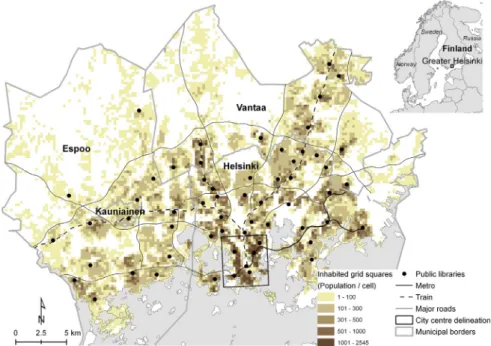
The empirical part of this paper takes place in Greater Helsinki, the capital region of Finland (Fig. 2). Greater Helsinki comprises
four municipalities and has approximately one million inhabitants. The highest population densities are found in the city centre of Helsinki and along suburban railway lines.
In 2008, 39% of daily trips in the Greater Helsinki area were done by car whereas the share of public transport trips was 26% (HRT, 2010). The road network of the region relies on a few large ring roads (west-east) and several radial roads originating from the city centre of Helsinki (Fig. 2). Congestion during the rush hour is concentrated on the area inside the inner ring road and on the radial roads leading to the city centre, and congestion charges are a hot topic in contemporary urban politics (Välipirtti et al., 2011). Parking is challenging particularly in the city centre (Kurri and Laakso, 2002).
The public transport system of Greater Helsinki relies on an extensive bus network and a few railway lines, complemented by trams and a metro within the municipality of Helsinki. In total, there are roughly 600 transit lines in the region (excluding service lines and night buses). Overall, the current structure of the public transport network is highly city centre oriented and crosstown connections are one of the key development areas of public trans-port planning.
4. Materials and methods
4.1. Study design
In order to test the comparability of travel time analyses by dif-ferent travel modes, we performed a set of routing analyses for
both car and public transport (Fig. 3). As route origins we used cen-troids of inhabited grid cells in Greater Helsinki. The alignment of the 250 m250 m cells corresponded to the Grid Database of Sta-tistics Finland (2012)and the inhabited grid cells were identified based on building-level population data in SeutuCD 2009 (Table 1). The routes’ destinations were 59 public libraries, which are one of the most actively used public services in Finland (Vakkari and Serola, 2012). Here, the type of destinations was fairly unimpor-tant, since the primary aim of this paper is to perform methodolog-ical comparisons – thus, rather than the type of facility, their spatial distribution was the main criterion for their selection. Pub-lic libraries are quite evenly distributed in the study area (Fig. 2) and thus provide a relatively representative sample of different areas around Greater Helsinki.
We calculated travel times and network distances between all origins and all destinations, using three different models for each travel mode, here named as simple, intermediate and advanced model. We also computed Euclidean distances between all origins and destination, in order to show how much more complicated real-life travel routes are in our study area in comparison to Euclid-ean distances which in many cases are used as accessibility surro-gates (e.g.Boscoe et al., 2012; Phibbs and Luft, 1995). The chosen grid cell resolution naturally affects the distance calculations (lar-ger grid cells leading to increased inaccuracy in results) and we deemed the 250-m cell to be sufficiently detailed for our purposes. With this grid cell size, the time needed for computations was rea-sonable, and yet, the positional error resulting from aggregation of the building level data was rather minor and did not have consid-wait
bus drive
O
walk P car drive search P walkD
O
walk S S walk S S walkD
wait bus drive O Origin D Destination P Parking space S TransitStop (a) Door-to-door by CAR:
(b) Door-to-door by PUBLIC TRANSPORT:
Fig. 1.Examples of the door-to-door approach in (a) car journeys and (b) PT journeys.
Fig. 2.Study area. Background mapÓThe City Survey Division of Helsinki, municipalities of Greater Helsinki, HSY, 01.01.2012.
erable effect on the accuracy of the distance (and time) calculations.
We compared travel times and distances between the different models by calculating their mutual ratios and correlations: For example, travel times produced by the simple and intermediate car models (see Section4.2) were compared for each origin–desti-nation pair by calculating the ratio between the two. These ratios were then averaged and the Pearson correlation coefficient was calculated to reveal how well the values produced by the different models correlated with each other. Similar assessments were done between all models, both for travel times and trip distances (including Euclidean distances).
Finally, travel time ratios between the travel modes (PT travel times divided by car travel times) were visualised as maps. 4.2. Car models
Thesimple car modelused the national road and street database Digiroad as the routing network dataset (Table 1). Each road seg-ment had a speed limit attributed to it, and these speed limits to-gether with the segment lengths determined the drive-through time of each segment. Digiroad was also used in theintermediate car modelbut the speed limit-based impedances were adjusted to fit the real-life driving times in the case study area. This was done by assigning cross roads a deceleration value which was different
for each road class (cf. Määttä-Juntunen et al., 2011; Thériault et al., 1999; Yiannakoulias et al., 2013). The deceleration values were derived from floating car measurements (for more on the floating car method, seeLi et al., 2011) where real travel speeds along different roads of the study area were measured during nor-mal weekdays in spring and autumn 2009, at different times of the day (data sources inTable 1). Based on a regression analysis, the effect of functional road classes and crossroads on travel speeds was formulated to deceleration values which in this case corre-sponded to average deceleration during a day (Jaakkola et al., in press). Crossroads on road classes 1 and 2 (regional main roads/ streets) got a daily average deceleration value of 11.31 s; cross-roads on road class 3 (local main streets/regional cross-roads) got 9.44 s; and crossroads on road classes 4–6 (collector streets/con-necting roads, feeder streets and private roads) got 9.36 s. Drive times were calculated using the Network Analyst extension in Arc-GIS 10 where the route optimisation was based on the fastest (not
necessarily the shortest) route between all origins and
destinations.
Theadvanced car modelwas built on the intermediate model but it also included the time spent walking from the point of origin to the parking space at the start of the journey, the time spent searching for a parking space at the destination, and, finally, the time spent walking from the parking space to the destination – in other words, the advanced model used the previously presented
door-to-door approach. We used empirical studies on parking con-ditions in the Greater Helsinki area and other city areas in Finland to determine the average walking distances between the point of origin and the parking space and between the parking space and the destination: in the city centre area the average distance was defined as 180 m and outside the city centre as 135 m (Kurri and Laakso, 2002). These were average distances for all types of parking spaces, and determined based on a survey that was conducted in May 2000 (most of the answers were gathered on normal week-days, but part of the answers during a Saturday) (Kurri and Laakso, 2002). We applied these distances both at the beginning of the journey (distance from the origin to the parking space) and at the end of the journey (distance from the parking space to the des-tination). Distances were then transferred as times, using a walking speed of 70 m/min which is a default value for walking speed in the Journey Planner route search application (see Section4.3) (HRT, 2011). The time spent in searching for a parking space at the des-tination was defined as 0.73 min, which is an average value for on-street parking on a normal weekday (Kalenoja and Häyrynen, 2003).
4.3. Public transport models
Thesimple PT modelwas based on a multimodal network data-set created in ArcGIS 10. In the datadata-set, public transport routes and their associated stops were grouped by travel mode, and each mode formed its own connectivity group in the network dataset. These groups were connected to each other through a pedestrian network represented by the Digiroad data (which contains pedes-trian roads in addition to roads for motorised transport). The time needed to cover each pedestrian segment was calculated using a walking speed of 70 m/min. Connections between the PT network and the pedestrian network were modelled by straight lines be-tween each PT stop and the closest edge element along the pedes-trian network (boarding/exit lines). Travel times by each mode were calculated based on an average speed of the respective travel mode (derived from route lengths and approximate route drive-through times on a normal weekday during the winter schedules) (Tables 1 and 2). Walking from the origin point to the closest PT
stop and walking from the last PT stop to the final destination were ignored, and the origin and destination locations were snapped di-rectly to the closest PT stop. The simple model also ignored transfer times.
Theintermediate PT modelused the same network dataset struc-ture and the same mode-specific average speeds as the simple model. It differed in that it accounted for transfer times: half a headway time was added to the in-vehicle travel time when the first PT vehicle was entered and if transfers occurred from one tra-vel mode to another. Headway times were mode-specific and based on average scheduled headway times around the morning rush hour (8 am) and outside rush hour (12 pm) on a regular week-day during the winter schedules (Table 2). In the network dataset, transfer times were assigned to the boarding lines.
The advanced PT model used the Journey Planner API (HRT, 2011), which contains data on up-to-date public transport routes and schedules in the study area. The PT schedules are planned to take into account congestion-related delays in route drive-through times. The databases of the API were queried using tools developed in-house (seeJäppinen et al., 2013; the source codes of the tools are available in Github https://github.com/matti/reittihaku). In or-der to account for the daily variation in schedules, we performed four route searches between each origin and destination, two dur-ing the rush hours and two outside the rush hours. Each route search resulted in three alternative route suggestions and the final travel times and distances are the average values of these 12 routes (4 timeslots3 route suggestions). The door-to-door approach is inherently included in the Journey Planner routes, which include the walk from the origin to the first PT stop, all the necessary PT
Table 1
Data sources.
Dataset Referencea
Description Phase of analysis
Driving speeds Helsinki Region Transport/Helsinki City Planning Office
Floating car measurements of real-life driving speeds along main roads
Preparation of intermediate and advanced car routing data Parking studies Kurri and Laakso (2002)/Kalenoja
and Häyrynen (2003)
Empirical studies on parking conditions in the Greater Helsinki area and other city areas in Finland
Preparation of advanced car routing data
Digiroad Finnish Transport Agency (2011) National road and street database Simple car model Modified
Digiroad
Jaakkola et al. (in press) Digiroad data modified to correspond to local driving conditions Intermediate and advanced car models
Public transport routes
SeutuCD (2009) Geometry of the public transport network in the Greater Helsinki area
Simple and Intermediate PT model Average PT route
times
Helsinki Region Transport (2012) Average route times for each public transport route Simple and intermediate PT model Average PT
headway times
Helsinki Region Transport (2012) Average headway times for each public transport mode Intermediate PT model
Journey Planner API
Helsinki Region Transport (2011) Application Programming Interface to Helsinki region public transportation timetable and route database
Advanced PT model Population
statistics
SeutuCD (2009) Building-level statistics on population in the study area, aggregated in 250250 m cells
OD-matrix (origins) Libraries Helmet libraries Location of public libraries in the Greater Helsinki area OD-matrix (destinations) SeutuCD (2009). Produced by Helsinki Region Environmental Services Authority.
Helsinki Region Transport (2012). http://www.hsl.fi/EN/timetablesandroutes/Pages/default.aspx. Helsinki Region Transport (2011). http://developer.reittiopas.fi/pages/en/home.php.
a Finnish Transport Agency (2011). http://www.digiroad.fi/en_GB/.
Table 2
Mode-specific average speeds and transfer times used in the simple and intermediate PT models.
PT travel mode
Average speed (km/h)
Transfer time (average headway time (min)/2)
Bus 26.3 12.3
Tram 13.3 4.7
Metro 39.9 4.5
Train 54.1 14.9
routes and transfers, and the walk from the last PT stop to the final destination. All route searches were performed using the winter schedules and a normal weekday. Route search settings were the default settings provided by the Journey Planner (e.g., walking speed 70 m/min) (for more detailed description of default values, seeHRT, 2011).
5. Results
5.1. Model comparisons within each mode
The differences between the models are illustrated inFig. 4, where a 20-min catchment area around a selected destination
(the main library) is drawn using all the models (4a: car models; 4b: PT models). In the simple car model, a majority of inhabited grid cells (5914) is reached within a 20-min drive. Within the same time, the intermediate car model reaches 1982 cells and the ad-vanced car model reaches 861 cells. The 20-min catchment areas in the PT models are much smaller than in the car models but there are notable differences between the PT models: the simple model reaches 985 cells, the intermediate model 85 cells and the ad-vanced, 234 cells.
When looking at trips from all origins to all destinations, corre-lations between all the models are high and statistically significant (>0.82**) (Table 3). In the car models, travel times in the advanced model are on average over twice as long as in the simple model. In
Fig. 4.20-min catchment areas around the main library produced by (a) car models and (b) PT models. Background mapÓThe City Survey Division of Helsinki, municipalities of Greater Helsinki, HSY, 01.01.2012.
Table 3
Pair-wise comparison of different models: Average ratios between median travel times and trip distances in the different models (Pearson correlations in parentheses).
Simple car Intermediate car Advanced car Simple PT Intermediate PT Advanced PT Euclidean distance
TT TD TT TD TT TD TT TD TT TD TT TD TD Simple car TT 1 (1.00**) TD (.972**) 1 (1.00**) Intermediate car TT 1.76 (.977**) (.938**) 1 (1.00**) TD (.973** ) 1.05 (.980** ) (.956** ) 1 (1.00** ) Advanced car TT 2.20 (.976**) (.934**) 1.24 (.998**) (.953**) 1 (1.00**) TD (.973**) 1.08 (.980**) (.956**) 1.03 (1.00**) (.954**) 1 (1.00**) Simple PT TT 2.18 (.928**) (.924**) 1.25 (.903**) (.914**) 1.02 (.903**) (.914**) 1 (1.00**) TD (.933**) 1.06 (.961**) (.901**) 1.02 (.942**) (.897**) 0.99 (.942**) (.928**) 1 (1.00⁄⁄ ) Intermediate PT TT 3.41 (.954**) (.969**) 1.94 (.928**) (.959**) 1.57 (.925**) (.959**) 1.61 (.953**) (.967**) 1 (1.00**) TD (.955**) 1.00 (.977**) (.927**) 0.96 (.962**) (.923**) 0.94 (.962**) (.925**) 0.95 (.972**) (.981**) 1 (1.00**) Advanced PT TT 3.53 (.869**) (.855**) 2.01 (.843**) (.847**) 1.62 (.847**) (.847**) 1.67 (.888**) (.861**) 1.04 (.878**) (.861**) 1 (1.00**) TD (.938**) 1.19 (.955**) (.912**) 1.14 (.939**) (.910**) 1.11 (.939**) (.946**) 1.14 (.960**) (.962**) 1.20 (.962**) (.919**) 1 (1.00**) Euclidean distance TD (.948** ) 0.72 (.974** ) (.916** ) 0.69 (.963** ) (.913** ) 0.68 (.963** ) (.907** ) 0.69 (.955** ) (.962** ) 0.73 (.973** ) (.830** ) 0.62 (.937** ) 1 (1.00** ) TT = Travel time. TD = Travel distance.
** Correlation is significant at the 0.01 level (2-tailed).
M. Salonen, T. Toivonen /Journal of Transport Geography 31 (2013) 143–153 149
comparison to the intermediate model, the advanced model travel times are less than 25% longer. Differences in trip distances are, at the most, 8% (advanced vs. simple car model).
In the PT models, travel times in the advanced model are nearly 70% longer than in the simple model. In comparison to the inter-mediate model, the advanced model travel times are 4% longer. Differences in trip distances are, at the most, 20% (advanced vs. intermediate PT model).
Euclidean distances are around 30% shorter than trip distances along the road network in all the models. The biggest difference
found was between the advanced PT model and Euclidean dis-tances: Euclidean distances account for up to 62% of trip distances in the advanced PT model.
5.2. Intermodal model comparisons
When travel modes are compared to each other, the largest dif-ferences in average travel times are found between the advanced PT model and the simple car model (PT travel times over 3.5 times as long as car times) (Table 3). When the supposedly conceptually
Fig. 5.Spatial distribution of travel time ratios in the (a) simple car and simple PT models; (b) intermediate models and (c) advanced models. Note that class intervals vary between maps. Background mapÓThe City Survey Division of Helsinki, municipalities of Greater Helsinki, HSY, 01.01.2012.
corresponding models are compared (i.e. simple PT vs. simple car; advanced PT vs. advanced car), differences in average travel times are smallest between the advanced models (PT travel times on average are 1.62 times longer than car travel times). Among the simple models the average travel times are 2.18 times longer by PT and among intermediate models 1.94 longer by PT.
In trip distances the largest difference between the travel modes is found between the advanced PT model and the simple car model (1.19 times longer trips in the PT model). When the cor-responding models are compared, the largest differences are found between the advanced models (on average 11% longer distances by PT).
The spatial distributions of modal travel time ratios are shown inFig. 5((a) simple models; (b) intermediate models; (c) advanced models). The grid cell values reveal how much longer PT travel times are on average when looking at journeys to all destinations from the respective origin cell.
The smallest differences between the simple car and simple PT models are concentrated along the railway lines, meaning that the PT travel times from these areas to all destinations are at the maximum twice as long as car travel times. Southern parts of the city centre area are characterised by smaller differences but otherwise the city centre area is a mixture of high and low ratios, which means that in some parts of the city centre the aver-age travel times by PT are up to 3.6 times longer than travel times by car. In the intermediate models, areas along the ring roads and in the inner city are characterised by high travel time ratios. Smaller values are found along the seashore in particular. In the advanced models, the city centre area has a considerable concen-tration of low ratios, meaning that in these models PT travel times are fairly competitive in relation to car travel times in the city centre. Other areas of low differences are found along the railway lines. The largest differences are concentrated along the edges of the study area, indicating that travelling by PT from these areas to the destinations is much slower than travelling by car.
Mean travel times are longer by public transport (36.1– 55.7 min) than by car (16.6.–34.4 min), no matter which models are used for comparison (Fig. 5, embedded tables). Travel times in the intermediate models are longer than in the simple models, and, correspondingly, the advanced models produced longer travel times than the intermediate models. Mean trip distance, in turn, appears shorter in the intermediate PT model in comparison to its corresponding car model (18.3 km vs. 19.4 km, respectively). Furthermore, the mean distance in the intermediate PT model is
shorter than in the simple PT model (18.3 km vs. 19.7 km, respec-tively). For comparison, the mean Euclidean distance is 13.5 km (standard deviation 7.0).
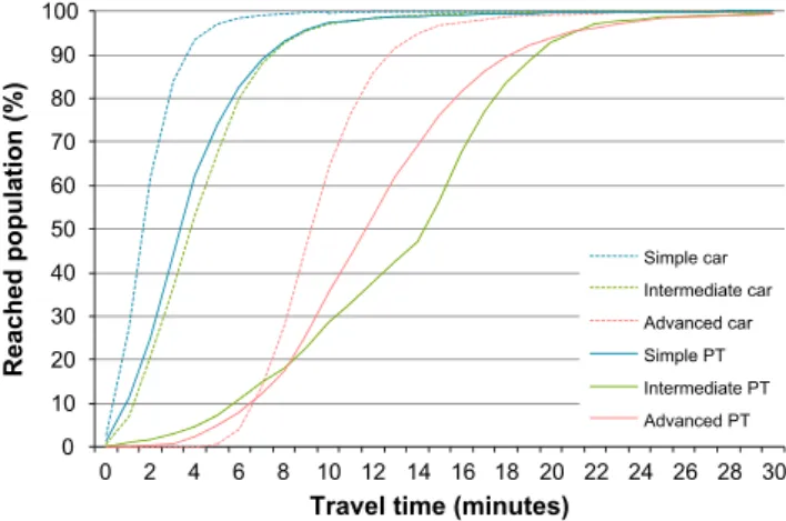
5.3. Travel time to the closest destination in the different models Cumulative travel time curves show how much time it takes for the city’s residents to get to their closest destination (Fig. 6). According to the simple car model, 95% of residents reach their closest destination in less than 5 min. The corresponding values in the intermediate and advanced car models are 9 min and 15 min, respectively. The simple PT model suggest that 95% of the population reach their closest destination in less than 9 min, while the corresponding value in both the intermediate and ad-vanced PT models is 21 min.
Differences in trip distances among the models are much smal-ler and not shown as figures.
6. Discussion
6.1. The comparability of travel modes
Advanced GIS methods, the availability of open data sources and increasing processing capacity allow accessibility analyses to be relatively easily incorporated into scientific work and practi-cal-level planning. With more modelling methods available, it is increasingly important to make sound methodological choices when conducting such analyses.
As we have demonstrated, it is essential to use conceptually corresponding models when comparing travel times between tra-vel modes. Modal comparison based on conceptually different models (e.g. advanced PT vs. simple car) may result in unrealisti-cally large differences; in our case study area, public transport might even appear to provide a much better level of accessibility than the private car (cf. simple PT vs. advanced car inFig. 6), which is seldom realistic in the Greater Helsinki area. If travel times are to be analysed in absolute terms, the approach taken by the more ad-vanced models presented in this paper is more reliable than the ap-proaches in the simple and the intermediate models: In PT journeys, access and egress times and delays related to transfers may make up a considerable share of the total travel time. Further-more, average speeds used by the simple and intermediate PT models ignore the effect of urban structural variables on speeds in different parts of the urban region. Similarly in the car models, congestion and time necessary for parking make the journeys last considerably longer and affect route choices too.
Travel time in urban surroundings is to a high degree dependent on the day of week and time of day (Lei and Church, 2010): thus, during weekdays and weekends and during rush hours and outside them the disparities between travel modes might appear some-what different. At the very least, the model elements in the concep-tually corresponding models should thus be based on the same day of week (as was the case in all our models). Indeed, the advanced models would allow a more detailed temporal analysis of accessi-bility disparity. The advanced PT model takes into account exact departure and arrival times and differences in route schedules that have been adjusted to traffic conditions at different times of day. Similarly, the deceleration values in the intermediate and ad-vanced car model could be adjusted to correspond to rush/non-rush hours. In our case, data on parking conditions (walking dis-tances and search times) were not detailed enough to allow for a temporal distinction but should such data be available, a temporal comparison of accessibility disparity could be carried out. This would definitively be an interesting theme for further examination. 0 10 20 30 40 50 60 70 80 90 100 0 2 4 6 8 10 12 14 16 18 20 22 24 26 28 30 Reached population (%)
Travel time (minutes)
Simple car Intermediate car Advanced car Simple PT Intermediate PT Advanced PT
Fig. 6.Cumulative share of residents accessing the closest library within a certain travel time (car models: dashed lines/PT models: continuous lines).
One common simplification in public transport travel time modelling is the use of half headway time as a surrogate for trans-fer-related waiting time. Results from our study area show that the intermediate model (applying this assumption) clearly underesti-mates travellers’ ability to optimise their journey: travel times on short journeys are considerably longer in the intermediate PT mod-el than in the advanced PT modmod-el (cf.Fig. 6), and one logical expla-nation is that transfer times in the advanced model – based on true schedules – are likely to be shorter than the half headway time would suggest. Owing to this, modal comparisons based on the intermediate models suggest unrealistically large modal disparities on short journeys.
As our results show, travel times are much more sensitive to the underlying model than trip distances. Travel times within each tra-vel mode get longer as the number of associated model elements (restricting rules) in the model grows. In terms of trip distances the effect of additional restricting rules may be different: PT trip distances were shorter in the intermediate than in the simple mod-el, mainly because the simple model can ‘‘afford’’ to make longer trips within the same time, as transfers between modes have no cost associated with them.
6.2. Findings on accessibility disparity
In the Greater Helsinki area, absolute differences in travel times between travel modes are notable – no matter which models are used for comparison. When conceptually corresponding models are compared, the relative modal differences are quite similar in the simple and intermediate models but considerably smaller in the advanced models.
These results partly challenge some recent findings:Benenson et al. (2011)found in Tel Aviv that the observed accessibility gap be-tween travel modes tends to grow if public transport analysis is done in more detail (using the door-to-door approach). Their public trans-port data takes into account walks at the start and end of the journey (though not in as much detail as in our advanced model) and their estimation of car travel times takes into account congestion but not parking (cf. our intermediate car model). Also in our data the modal disparity is larger if the intermediate car model is compared to the intermediate or advanced PT models than if the comparison is with the simple PT model. However, the difference between travel modes actually becomes smaller if both car and PT calculations are done at the most detailed level: in the advanced car model, park times considerably lengthen the total travel time, particularly in areas where public transport connections are at their best. Thus, the observed modal disparity in the advanced models becomes smaller than in the intermediate or simple models.
We further demonstrated that different parts of the study area get highlighted as areas for small/large accessibility disparity by the different models. Previous findings on modal accessibility dis-parity in an urban structure are to some degree controversial. Kawabata (2009)found the modal differences to be smallest in the downtown areas of Boston and San Francisco, and Elldér et al. (2012)demonstrated a similar pattern in Göteborg. In con-trast,Hess (2005)found the modal difference in job accessibility to be higher among downtown residents in Buffalo and Niagara Falls than in the suburbs. In the Greater Helsinki area, the compar-ison based on the advanced models intuitively produced the most reliable results since it recognised both the city centre and the proximity of railway lines as zones of lower accessibility disparity and the outer ring road as a zone of higher accessibility disparity. Given the relatively strong city centre orientation of the current transit system in the Greater Helsinki area and the challenging parking conditions within the city centre area, it follows that our study area falls into the category of cities where the gap is smaller in the city centre than outside it.
7. Conclusions
Using conceptually corresponding models for car and PT travel time calculations is the key to achieving a more reliable analysis of modal accessibility disparity. Furthermore, the door-to-door ap-proach in travel time calculations also makes the results truly com-parable in absolute terms. In all, the most detailed analyses of accessibility disparity seem to be possible only with the more ad-vanced models. Clearly, these models are also the most data hun-gry and accordingly, possibilities of using such models depend among other things on data policies of transport-related data pro-viders. In our case, the European INSPIRE initiative (http://inspir-e.jrc.ec.europa.eu/) and general development towards openness in data policies among public administration have markedly in-creased the possibilities of analysing multi-modal transport. How-ever, certain simplifications – such as the average park search times in our case – might be necessary if better data sources are lacking.
Requirements of the advanced PT model (e.g. inclusion of exact departure/arrival time and various route optimisation settings) may be overwhelming for a standard user to implement in a stan-dard GIS. Thus, not only open data but also open route search inter-faces (such as the Journey Planner API) providing the necessary algorithms and computational resources on servers, make such massive analysis feasible. Indeed, reliable spatial analyses of mul-timodal transport — which for long have been too data hungry and computationally intensive to calculate over large extents — are now more realistic for a larger group of researchers and practi-tioners than what they used to be.
Acknowledgements
We thank Helsinki Region Transport for providing their data freely, Matti Paksula for coding the query tools for the Journey Planner API and the two anonymous reviewers for constructive comments on the manuscript. We also thank the members of the MetropAccess-group: Timo Jaakkola for developing the modified Digiroad data, Jaani Lahtinen for helping with data gathering and Sakari Jäppinen for commenting the manuscript at various phases. KatuMetro research program and University of Helsinki have funded the research work.
References
Benenson, I., Martens, K., Rofé, Y., Kwartler, A., 2011. Public transport versus private car GIS-based estimation of accessibility applied to the Tel Aviv metropolitan area. Annals of Regional Science 47 (3), 499–515.
Bertolini, L., le Clercq, F., Kapoen, L., 2005. Sustainable accessibility: a conceptual framework to integrate transport and land use plan-making. Two test-applications in the Netherlands and a reflection on the way forward. Transport Policy 12 (3), 207–220.
Boscoe, F.P., Henry, K.A., Zdeb, M.S., 2012. A nationwide comparison of driving distance versus straight-line distance to hospitals. Professional Geographer 64 (2), 188–196.
Christie, S., Fone, D., 2003. Equity of access to tertiary hospitals in Wales: a travel time analysis. Journal of Public Health Medicine 25 (4), 344–350.
EEA – European Environment Agency. 2006. Urban sprawl in Europe. The ignored challenge. EEA Report 10/2006, 1–56.
Elldér, E., Solá, A.G., Larsson, A., 2012. Featured graphic. Spatial inequality and workplace accessibility: the case of a major hospital in Göteborg, Sweden. Environment and Planning A 44 (10), 2295–2297.
Eluru, N., Khakour, V., El-Geneidy, A., 2012. Travel mode choice and transit route choice behaviour in Montreal: insights from McGill University members commute patterns. Public Transport 4 (2), 129–149.
Filion, P., 2000. Balancing concentration and dispersion? Public policy and urban structure in Toronto. Environment and Planning C: Government and Policy 18 (2), 163–189.
Frank, L., Bradley, M., Kavage, S., Chapman, J., Lawton, T.K., 2008. Urban form, travel time, and cost relationships with tour complexity and mode choice. Transportation 35 (1), 37–54.
Hepinstall-Cymerman, J., Coe, S., Hutyra, L.R., 2013. Urban growth patterns and growth management boundaries in the Central Puget Sound, Washington, 1986–2007. Urban Ecosystems 16 (1), 109–129.
Hess, D.B., 2005. Access to employment for adults in poverty in the Bufallo-Niagara region. Urban Studies 42 (7), 1177–1200.
HRT – Helsinki Region Transport. 2010. Helsingin seudun työssäkäyntialueen laajan liikennetutkimuksen (LITU 2008) yhteenveto. Helsinki: Edita Oy. <http:// www.hsl.fi/FI/mikaonhsl/julkaisut/Documents/2010/
Hgin%20seudun%20laajan%20liiktutk%20LITU%202008%20yhteenveto.pdf> (In Finnish) (accessed 12.03.13).
HRT – Helsinki Region Transport. 2011. Journey Planner API. <http:// developer.reittiopas.fi/pages/en/home.php> (accessed 12.03.13).
Jaakkola, T., Tenkanen, H., Toivonen, T., in press. MetropAccess-Digiroad. In: Toivonen et al. (Eds.), MetropAccess: Helsingin metropolialueen moniulotteista saavutettavuutta tutkimassa. in press. Helsingin yliopiston Geotieteiden ja maantieteen laitoksen julkaisuja C8, (in Finnish).
Jäppinen, S., Toivonen, T., Salonen, M., 2013. Modelling the potential effect of shared bicycles on public transport travel times in Greater Helsinki: An open data approach. Applied Geography 43, 13–24.
Kalenoja, H., Häyrynen, J.-P., 2003. Keskustan pysäköinti osana liikennejärjestelmää – Tampereen keskustan pysäköintitutkimus. Tampere: Tampere University of Technology. <http://www.tut.fi/verne/wp-content/uploads/ tampereen_keskustan_pysakointitutkimus.pdf> (in Finnish, abstract in English) (accessed 12.03.13).
Kawabata, M., 2003. Job access and employment among low-skilled autoless workers in US metropolitan areas. Environment and Planning A 35 (9), 1651– 1668.
Kawabata, M., 2009. Spatiotemporal dimensions of modal accessibility disparity in Boston and San Francisco. Environment and Planning A 41 (1), 183–198.
Kawabata, M., Shen, Q., 2007. Commuting inequality between cars and public transit: The case of the San Francisco Bay Area, 1990–2000. Urban Studies 44 (9), 1759–1780.
Kurri, J., Laakso, J.-M., 2002. Parking policy measures and their effects in the Helsinki metropolitan area. The Helsinki Metropolitan Area Publication Series C 2002:18. Helsinki: Helsinki Metropolitan Area Council (YTV) (in English and Finnish).
Kwok, R.C.W., Yeh, A.G.O., 2004. The use of modal accessibility gap as an indicator for sustainable transport development. Environment and Planning A 36 (5), 921–936.
Lei, T.L., Church, R.L., 2010. Mapping transit-based access: integrating GIS, routes and schedules. International Journal of Geographical Information Science 24 (2), 283–304.
Levinson, D.M., 1998. Accessibility and the journey to work. Journal of Transport Geography 6 (1), 11–21.
Li, Q., Zhang, T., Wang, H., Zeng, Z., 2011. Dynamic accessibility mapping using floating car data: A network-constrained density estimation approach. Journal of Transport Geography 19 (3), 379–393.
Liu, S., Zhu, X., 2004. Accessibility analyst: an integrated GIS tool for accessibility analysis in urban transportation planning. Environment and Planning B: Planning and Design 31 (1), 105–124.
Lovett, A., Haynes, R., Sünnenberg, G., Gale, S., 2002. Car travel time and accessibility by bus to general practitioner services: a study using patient registers and GIS. Social Science and Medicine 55 (1), 97–111.
Määttä-Juntunen, H., Antikainen, H., Kotavaara, O., Rusanen, J., 2011. Using GIS tools to estimate CO2emissions related to the accessibility of large retail stores in the Oulu region, Finland. Journal of Transport Geography 19 (2), 346–354.
Martin, D.J., Wrigley, H., Barnett, S., Roderick, P., 2002. Increasing the sophistication of access measurement in a rural healthcare study. Health and Place 8 (1), 3–13.
Martin, D.J., Jordan, H., Roderick, P., 2008. Taking the bus: Incorporating public transport timetable data into health care accessibility modelling. Environment and Planning A 40 (10), 2510–2525.
Mavoa, S., Witten, K., McCreanor, T., O’Sullivan, D., 2012. GIS based destination accessibility via public transit and walking in Auckland, New Zealand. Journal of Transport Geography 20 (1), 15–22.
Moniruzzaman, M., Páez, A., 2012. Accessibility to transit, by transit, and mode share: application of a logistic model with spatial filters. Journal of Transport Geography 24, 198–205.
O’Sullivan, D., Morrison, A., Shearer, J., 2000. Using desktop GIS for the investigation of accessibility by public transport: an isochrone approach. International Journal of Geographical Information Science 14 (1), 85–104.
Peipins, L.A., Graham, S., Young, R., Lewis, B., Foster, S., Flanagan, B., Dent, A., 2011. Time and distance barriers to mammography facilities in the Atlanta metropolitan area. Journal of community health 36 (4), 675–683.
Phibbs, C.S., Luft, H.S., 1995. Correlation of travel time on roads versus straight line distance. Medical Care Research and Review: MCRR 52 (4), 532–542.
Shen, Q., 2001. A spatial analysis of job openings and access in a US metropolitan area. Journal of the American Planning Association 67 (1), 53–68.
Silva, C., Pinho, P., 2010. The structural accessibility layer (SAL): revealing how urban structure constrains travel choice. Environment and Planning A 42 (11), 2735–2752.
Statistics Finland. 2012. Grid database. <http://www.stat.fi/tup/ruututietokanta/ index_en.html> (accessed 2.06.13).
Thériault, M., Vandersmissen, M.H., Lee-Gosselin, M., Leroux, D., 1999. Modelling commuter trip length and duration within GIS: application to an O–D survey. Journal of Geographic Information and Decision Analysis 3 (1), 41–55.
Tribby, C.P., Zandbergen, P.A., 2012. High-resolution spatio-temporal modeling of public transit accessibility. Applied Geography 34 (4), 345–355.
Vakkari, P., Serola, S., 2012. Perceived outcomes of public libraries. Library and Information Science Research 34 (1), 37–44.
Välipirtti, K., Suvanto, T., Moilanen, P., 2011. Helsinki Region Congestion Charges.Summary and conclusions. (English summary of the publication). Publications of the Ministry of Transport and Communications 5/2011. <http:// www.lvm.fi/c/document_library/get_file?folderId=1551284&name=DLFE-11740.pdf&title=Helsinki%
20Region%20Congestion%20Charges_English%20Summary> (accessed 15.01.13).
Yiannakoulias, N., Bland, W., Svenson, L.W., 2013. Estimating the effect of turn penalties and traffic congestion on measuring spatial accessibility to primary health care. Applied Geography 39, 172–182.