Burst pressure estimation of corroded pipeline with interacting defects using FEA

Burst pressure estimation of corroded pipeline with interacting defects using FEA

by

Ahmad Shakir bin Aminudin

Dissertation submitted in partial fulfillment of tbe requirements for the

Bachelor of Engineering (Hons) (Mechanical Engineering)

September 20 II

Universiti Teknologi PETRONAS Bandar Seri Iskandar

3I750 Tronoh Perak Darui Ridzuan

CERTIFICATION OF APPROVAL

Burst pressure estimation of corroded pipeline

with interacting defects using FEA

by

Ahmad Shakir bin Aminudin (10606)

A Project Dissertation submitted in partial fulfilment of the requirements for the

Bachelor of Engineering (Hons) (Mechanical Engineering)

SEPTEMBER 2011

UNIVERSITJ TEKNOLOGI PETRONAS TRONOH, PERAK

CERTIFICATION OF ORIGINALITY

This is to certifY that I am responsible for the work submitted in this project, that the original work is my own except as specified in the references and acknowledgements, and that the original work contained herein have not been undertaken or done by unspecified sources or persons.

ACKNOWLEDGEMENT

In the name of Allah, The Most Gracious, The Most Merciful. Praise to Allah S. W. T by whose grace and sanction I manage to complete Final Year Project within time.

I would like to extend my sincere gratitude to my supervisor Dr. Saravanan Karoppanan who has given me. advices, opinions and guides in completion of this project Through his kindness and precious moment, I manage to face all the problems that been encountered during these whole period. Thank you .again for the knowledge sharing.

Not forgetting to other lecturers of UTP especially from the Mechanical Engineering department, thanks for useful thoughts and assistance that help me a lot in completing this project.

Last but not least, to my parents and colleagues for the supports given during the completion of this project.

ABSTRACT

Failure due to corrosion defects has been the major problem in maintaining pipeline's integrity. The loss ofmetal due to corrosion usually results in localized pits with various depth and irregular shapes which occur on its external and internal surfaces. An interacting defect is one that is located sufficiently close and able to interact with neighboring defects in an axial or circumferential direction. The maximum allowable pressure that can be sustained in a pipeline with interacting. defects is lower than it is in single defects due to interaction of neighboring defects. There are several methods available to assess the corrosion metal loss defects in order to evaluate Fitness-for-Services (FFS) of the corroded pipeline. In this study, finite element simulations will be carried out to determine the maximum allowable burst strength of corroded pipeline with interacting defects. The finite element analysis (FEA) results show that failure pressure of corroded pipeline with interaeting defects are higher than empirical values gained from DNV-RP-F!Ol Code,

TABLE OF CONTENTS CERTIFICATION OF APPROVAL. CERTIFICATION OF ORIGINALITY. ABSTRACT. ACKNOWLEDGEMENT CHAPTER I: CHAPTER2: CHAPTER3: INTRODUCTION 1.1. Background of Study . 1.2. Problem Statements .

1.3. Objectives and Scope of Study.

LITERATURE REVIEW 2.1 Pipeline Corrosion 2.2 Interacting Defects 2.3 Offset Defects .

2.4 Finite Element Analysis.

METHODOLOGY .

3.1. Research Methodology. 3.2 DNV-RP-FIOl

3.3 Modeling in ANSYS

3.3.1 Defining element types . 3.3.2 Defming material properties 3.3.3 Creating model geometry 3.3 .4 Meshing . 3.3.5 Load 3.3.6 Analysis. 3.3.7 Comparison of Results 3.4 PmjectGanttchart ii iii iv 1 1 2 3 4 4 4 7 8 10 10 11 12 12 13 14 15 16 17 18 19

CHAPTER4: RESULTS AND DISCUSSIONS. 20

4.1 DNV Code Results

20

4.1.1

Allowable Corroded Pressure for Single

Defects, pi and p2

21

4.1.2

Allowable Corroded Pressure for Interacting

Defects, P nm

21

4.1.3

Maximum Allowable Corroded Pressure, Pcorr

23

4.2

Overall Result Summary.

24

CHAPTERS:

CONCLUSION AND RECOMMNEDATION.

34

5.1

Conclusion

34

5.2

Recommendation

34

LIST OF FIGURES

Figure 2.1 : Combined length of all combination of adjacent defects.

Figure 2.1 : Projection of overlapping defects onto a single projection line • Figure 3.1 : Process flow of the project

Figure 3.2 : Defming the element types of model Figure 3.3 : Defming nonlinear properties of model • Figure 3.4 : Engineering Stress vs. Strain graph for X65.

Figure 3.5 :Creating model by partial annulus on workplane Figure 3.6: Half ofthepipewith defect

Figure 3.7: Mapped mesh of the pipe

Figure 3.8 : Symmetry Boundary Conditons of the model. Figure 3.9 : Fixed end at all DOF (enclosed end)

Figure 3.1&: Internal load applied on pipe model

Figure 3.11 : Contour plot of Von Mises Stress distribution along the pipe . Figure 4.1 :Graph of Normalized corroded pressure, P corr(MPa) I Pintact(MPa) vs

spacing per square root of unit depth with thickness, ~ , for d/t = 0.1 • ..;Dxt

Figure 4.2 : Graph of Normalized corroded pressure, Pcore (MPa) I Pintact (MPa) vs spacing per square root of unit depth with thickness, ~ , for d/t = 0.2 .

vDxt

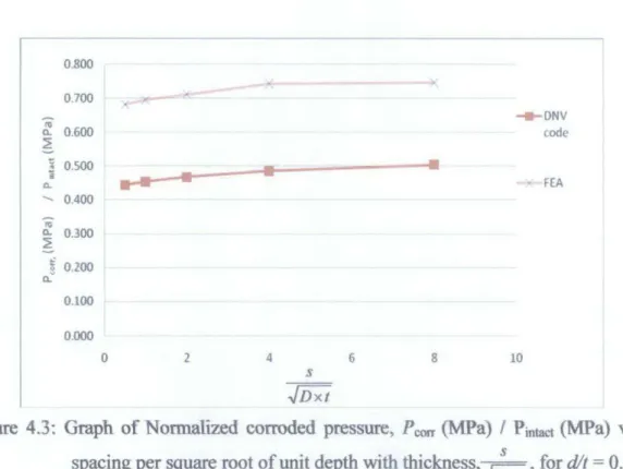
Figure 4.3 : Graph of Normalized corroded pressure, P corr (MPa) I Pintact (MPa) vs spacing per square root of unit depth with thickness, ~,for d/t = 0.3.

..;Dxt

Figure 4.4 : Graph ofNormalized corroded pressure, Pcorr (MPa)

I

Pintact (MPa) vs spacing per square root of unit depth with thickness, ~ , for d/t = 0.4 .

-vDxt

Figure 4.5 : Graph of Normalized corroded pressure, Pcore (MPa) I Prntact (MPa) vs spacing per square root of unit depth with thickness, ~ , for d/t = 0.5 .

..;Dxt

Figure 4.6 : Graph of Normalized corroded pressure, Pcore (MPa) I Pintact (MPa) vs spacing per square root of unit depth with thickness, ~ , for d/t = 0.6 •

-vDxt

Figure 4.7 :Graph of Normalized corroded pressure, P core (MPa) I Pintact (MPa) vs spacing per square root of unit depth with thickness, ~,for d/t = 0.7.

-vDxt

Figure 4.8 : Graph of Normalized corroded pressure, P corr (MPa) I Pintact (MPa) vs spacing per square root of unit depth with thickness, ~, for d/t = 0.8 •

-vDxt

Figure 4.9 : Graph ofNormalized corroded pressure, P core (MPa) I Pintact (MPa) vs spacing per square root of unit depth with thickness, ~ , for the FEA

..;Dxt 6

8

10 12 13 l3 14 15

15

16

16 17 17

25

25

26

27

27

28

29

29

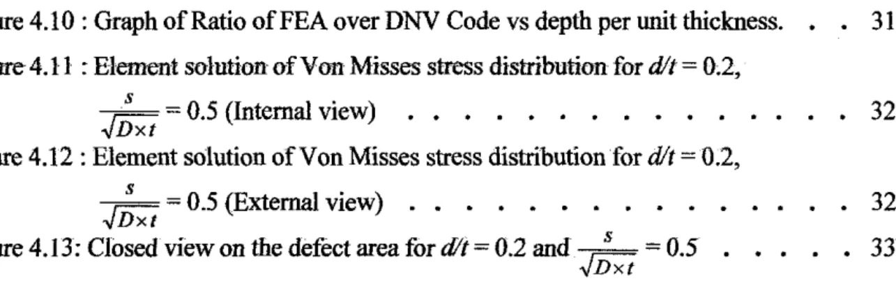
Figure 4.10: Graph of Ratio ofFEA over DNV Code vs depth per unit thickness. • • 31 Figure 4.11 : Element solution of Von Misses stress distribution for d/t =

02,

~ = 0.5 (Internal view) . • • . • . . . • • . . . . • 32

..;Dxt

Figure 4.12 : Element solution of Von Misses stress distributionfor d/t = 0.2,

~ = 0.5 (External view) . • • • • • . . • • 32

..;Dxt

Figure 4.13: Closed view on the defect area ford/t= 0.2 and ~ = 0.5 . • 33

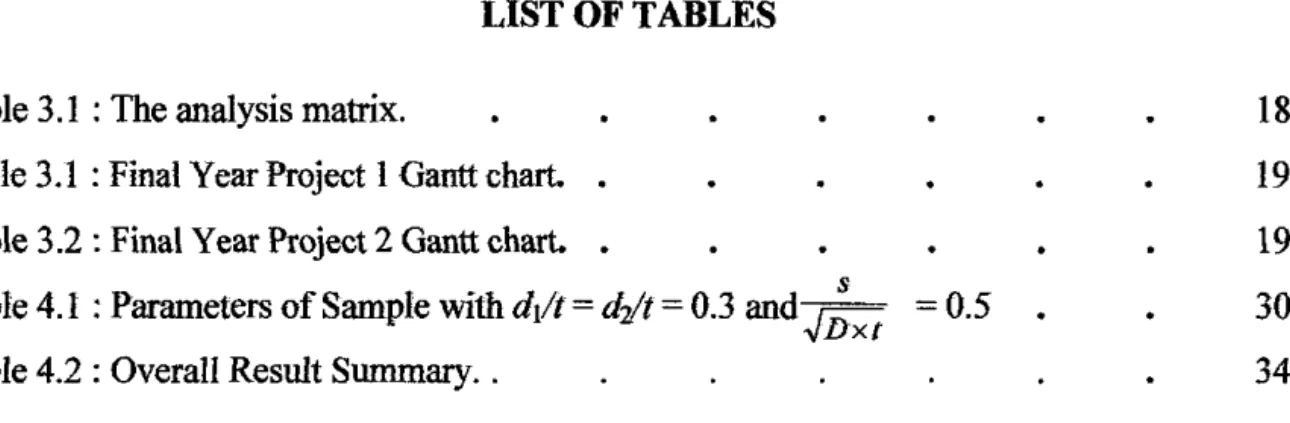
LIST OF TABLES Table 3.1 : The analysis matrix.

Table 3.1 : Final Year Project I Gantt chart. Table 3.2 : Final Year Project 2 Gantt chart.

Table 4.1 :Parameters of Sample with d1/t= d1ft

=

0.3 and

,J~xt

=

0.5 Table 4.2 : Overall Result Summary ..

18 19 19 30 34

CHAPTERl

INTRODUCTION

Pipeline systems are generally a convenient means for transferring oil and gas onshore or offshore due to the economic and safety reasons. However, with increasing age, the pipeline integrity can be affected by a range of corrosion mechanism.

Pipeline is exposed to both internal and external corrosion. The internal corrosion of pipeline is due to the harsh condition of hydrocarbon fluid; the presence of C02, H2S, organic acid and etc. While external corrosion occurs due to extreme condition of the surrounding environment in the event of failed preventive measures; older, degraded coat, or poorly coated pipeline [t, 21• This will result in metal loss at corroded location in

the pipeline and eventually may lead to its failure. The structural integrity assessment of corroded pipeline has become vital and the main interest to assist engineers to take wise decision toward replacing or repairing a pipeline. It is essential to ensure the continued safe operation and non hazardous occurrences which might affect the life and the environment.

1.1 Background ofstudy

An interacting defect is defined as the one that interacts with neighboring defects in an axial or drcumferential direction [31• As the extent of space between corrosion defects decrease up to certain distance, they will begin to interact reducing the maximum allowable pressure that can be sustained in a pipeline. The objective of this project is to estimate the burst pressure of corroded pipeline due to interacting corrosion defects by the means of FEA. The analysis is performed by nonlinear FEA simulation using ANSYS Software. This project will study on the effect of different spacing between two defects aligned in longitudinal direction and their failure pressure. Then the results of the FEA will be compared to the numerical values gained from the DNV RP-FlOlcode.

1.2 Problem Statement

The impact of corroded pipeline problems cause economic consequences; reduced operating pressure, loss of production due to downtime, repairs or replacement, and consequently increase of costs. Thus, there are several pipelines systems kept in operation even though they have shown signs of corrosion based on the data obtain from the corrosion management, inspection, and monitoring system (i.e.: intelligent pig). The continued operations of these pipelines are basically after determining the FFS assessment for their residual strength and recalculating the maximum allowable internal pressure of the product being transferred [41. The effect of pipeline burst strength of interacting defects will be lower than it is in single defects. A more reliable defect assessment method is needed due to the conservatism involved in the available assessment method l51• This is an approach to understand the effect of interacting defects toward the pipeline burst strength in a more reliable and convenient method other than performing the experimental testing. Therefore, the modeling of the problem using the FEA method can assist engineers to assess the burst strength of pipeline with interacting defects.

1.3 OBJECTIVE AND SCOPE OF STUDY

The objectives of this project are:

• To assess the burst strength of corroded pipelines due to interacting defects. • To compare the results from FEA with numerical values obtained from the

available codes.

The scope of this project will be simplified as follows: • The material of the pipelines is API SL X65.

• Results from FEA will be compared with empirical solutions provided by DNV-RP-FHH code.

2.1 Pipeline Corrosion

CHAPTER2

LITERATURE REVIEW

Unprotected pipelines are subjected to corrosion as well as when their corrosion preventions failed. Corrosion is defmed as the destruction or deterioration of a material because of its reaction with the environment [61. Corrosion defects in pipelines are assessed as metal loss defects that occur on the interior or exterior of pipeline surfaces. And if no appropriate maintenance actions taken, the location of corrosion become deteriorate. This consequently reduce the structural integrity of the pipeline hence can cause catastrophic failure of the system [71. For many years, various methods for assessing pipeline corrosion are available and commercially have been practiced by the industry; such as ANSIIASME B31G [SJ. For more realistic way of pipeline corrosion representation [91, new criteria are developed, such as RSTRENG Effective Area [lOJ, and DNV RP-F 101 [31• These methods include the specification dealing with the effects of the interacting defects. Even though these codes have been used widely for assessing the integrity of in-service pipelines, they are known to be conservative [llJ_ Meaning that, pipelines which have been assessed by these codes for the purpose of FFS analysis probably lead to either unnecessary maintenance or premature replacement.

2.2 Interacting Defects

The occurrence of corrosion is divided into several categories; individual pits, colonies of pits, general wall-thickness reduction, or in ~ombinations [IZJ_ For colonies of corrosion defects, as the distance between the defects decreases, they will begin to interact and resulting in reduced burst strength of the pipe. DNV-RP-FIOI method for interacting defects (part A) will be used in this study to estimate the burst pressure of the corroded pipeline. In DNV procedure, all the defects that are supposed to interact are

projected onto a longitudinal line. The metal loss is represented by the maximum defects depth and the projected defects length.

In the case of overlapped defects, they are combined to form composite defect The formation of combined defects is estimated by taking the combined length and the depth of the deepest defect. For combination of overlapping internal and external defect, the depth of the composite defect is the sum of maximum depth of those two defects.

Each defect or composite defects (i) with length (/;) and depth (d;) is treated as a single defect and failure pressure ( p ;) is defined based on the expression below:

. 2tfu(l-}fl(dil t)*)

PI= '}'m ( yd(di

It)*)

j = !, ... , N

(D-t) 1-

~---''-Q;

(2.1)

where N is the is number of projected defects, D is the nominal outside diameter (mm), t is uncorroded measured pipe wall thickness or t110m (mm),

fu

is the ultimate tensile

strength, yd is the partial safety factor for corrosion depth and Qi, is the length correction factor for individual defect, given by:

( )

_/,

'

Q; == }+0.31

.[D;

(2.2)

The correction depth over thickness ratio is determined by the following expression: (d1 /f)*= (di /f)mea' + &StD(d;/ f)

fu

= Minimum yield strength of the material

Ym

= Partial safety factor for model prediction

Yd

= Partial safety factor for corrosion depth

& = Factor for defining fractile value for the corrosion depth StD(d/t] =Standard deviation of the measured (d/t) ration

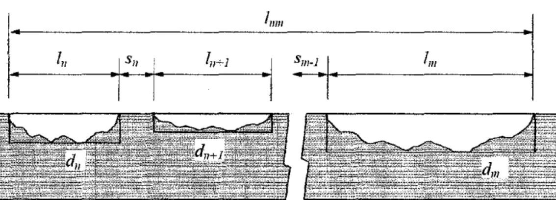
Next, the combinations of adjacent defects are investigated. Take note that for combined defects; the effective length (lnm) is the total length of the projected defects and the spacing between the defects (Figure 2.2). For defects from

n tom,

the effective length is given by

i=m-1

fnm=/m+

~)/;+s;)

n, m = J, ... ,N, (2.4)

i=n

where S; is the projected distance between the two adjacent defects.

Meanwhile, the effective depth (dnm) of combined defect formed from all of interacting defects from n tom (Figure 2.1} is calculated as below:

(2.5)

The failure pressure ( p nm) of the combined defects from n to m is calculated by replacing{/;)and (d;)with{lnm) and (dnm)in Eqs. {2.1) and (2.2) respectively.

Where the abbreviations are represented by the following:

=

ln =

Total longitudinal length of a defect combined with the adjacent defects n to m including spacing in between them (mm).

Longitudinal length of an individual defect (mm). s. = Longitudinal spacing between adjacent defects (mm). dn = Depth of corroded region (mm),

The minimum value, calculated for all single and combined defects, is taken as the failure pressure for the current projection line.

I :

111111

:I

!,

Is, .

ln-d

·I

Sm-1

I

lm

.. ·l

.

.

..

Figure 2. I: Combined length of all combination of adjacent defects

According to the DNV interaction rules, there is no interaction if the longitudinal (s1) and circumferential (sc) distances between defects satisfy the following conditions:

St > 2.0

.Jl);

2.3 Offset Defects

In real life problem, the corrosion does not occur rigidly in one location on the wall of the pipeline, instead, the corrosion attack the surface randomly which create colony of defects that are scattered on the attacked location. The defects in the colony may be overlapped or offset to one another. According to DNV code, simplification had been made for cases of multiple defects which were overlapped or offset conditions. The overlapped defects are combined together to form composite defect. This composite defect is projected onto a single projection line (Figure 2.2).

D

Projection Line

l

IY

iY

J

'

'

t

I I

I

'· ...

-

. . - ·· .. _j _,

I

'

. ~-. i ) ' \ j

...

. -.

.,___ Section Through Projection Line -'

I, s,

Figure 2.2: Projection of overlapping defects onto a single projection line

The simplification made on the DNV code does not take into consideration the offset condition of the interacting defect. In other word, the effect of offset between the

interacting defects is negligible in the DNV calculation.

2.4 Finite Element Analysis

The FEM is a powerful technique to simulate the linear and nonlinear behavior of structures. In order to have this method to be able to correctly evaluate the corroded pipe, appropriate failure criterion should be established to decide the failure point during the simulation rsJ. Resear<:h was done by Lee et. a/ flZJ to predict the failure pressure for multiple corroded defects on gas pipeline made of API 5L X65 steel by means of burst testing and FEM. 3D-elastic plastic finite element simulation has been performed using ABAQUS. Multiple corrosion defects were conceived as pits with equal profile defects with size of length (50mm), width (50mm), and depth (8. 75mm). These defects were aligned in longitudinal and circumferential directions. From the findings, comparison

between the burst tests and the finite element predictions showed that burst pressure had decreased with increased number of pits for longitudinal aligned defects. As for circumferential aligned defects, no significant change in burst pressure as distance between defects change.

Another study done by Silva et. al [91 on the assessment of pipe with interacting defects by FEM and neural networks application. The neural network is a mathematical algorithm which enables to relate the inputs and outputs parameters to establish the standard procedure for that particular process. The results from the finite element simulation were utilized as the databases for the neutral networks system. The material been used was API SL X52 steel. The defects are represented by two equally shaped defects of 80 mm x 32 mm with varied defect depth and separated by different defect spacing. These defects were aligned in longitudinal and circumferential directions. The results from the study showed that for case of longitudinal direction, specifically for closely space defect, relative pipe pressure capacity (ratio between failure pressure of multiple defect and single defect) reduced as depth of defect increased. On the contrary, for case of circumferential direction, little interaction of defects was observed which gave insignificant impact on the relative pipe pressure capacity.

CHAPTER3

METHODOLOGY

3.1 Research Methodology

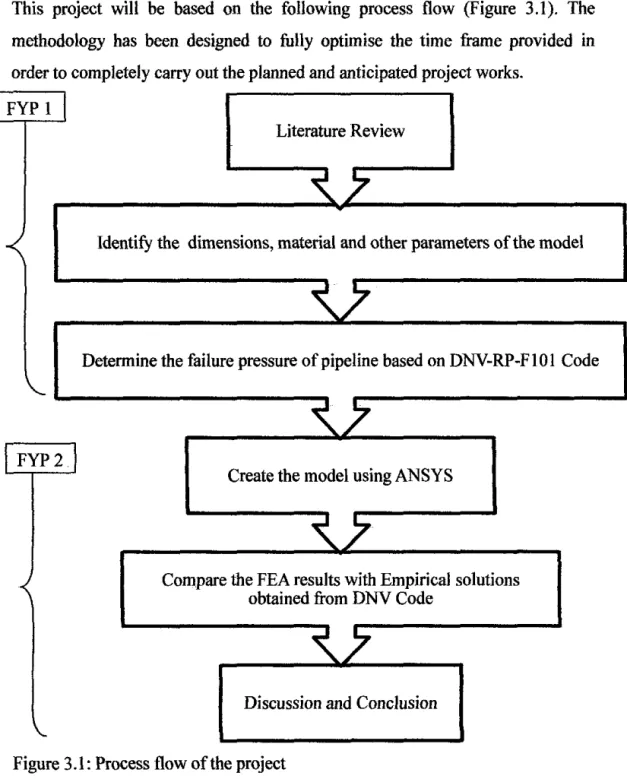
This project will be based on the following process flow (Figure 3.1). The methodology has been designed to fully optimise the time frame provided in order to completely carry out the planned and anticipated project works.

I

Literature Review

_S.7

Identify the dimensions, material and other parameters of the model

Q_

Determine the failure pressure of pipeline based on DNV-RP-FIOI Code

'<...7

2j

Create the model using ANSYS FYP

~7

Compare the FEA results with Empirical solutions obtained from DNV Code

'<...7

Discussion and Conclusion

3.2 DNV-RP-FlOl

Firstly, the empirical correlation provided in DNV-RP-FIOI code is studied. The related parameters such as depth of defects, spacing between defects, diameter of the pipeline, and length of the defects are determined by manipulating the correlation. The allowable corroded pressure of interacting defects is estimated using the following procedure:

3 .I.l The length of the defect is determined from the ratio between defect length and diameter of pipeline,

II D.

3.1.2 The allowable pipe corroded pressure (p~, pz...[JN) of each defect, or combined defect is calculated by using equation (2.1 ). The length correction factor is calculated based on equation (2.2). The failure pressure of the single defect will be chosen as the reference pressure. 3.1.3 The length between the defects is determined from the ratio between

spacing of the defects and square root of diameter and thickness of the

pipe,~

Dxt

3.1.4 Afterward, all combinations of adjacent defects are calculated. The combined length is calculated using equation (2.4).

3.1.5 Then, the effective depth of the combined defects is calculated based on equation (2.5).

3.1.6 The allowable corroded pipe pressure of the combined defect (pnm) is determined from equation (2.1) by replacing (/;) and (d;) with (/nm) and (dnm) in equation (2.1) and (2.2) respectively. The term (d;) in equation (2.3) is replaced with (dnm).

Several assumptions have been made in this study, firstly, the length of both defects that are supposed to interact are equal. Secondly, the interacting defects are considered between defects with similar depth only.

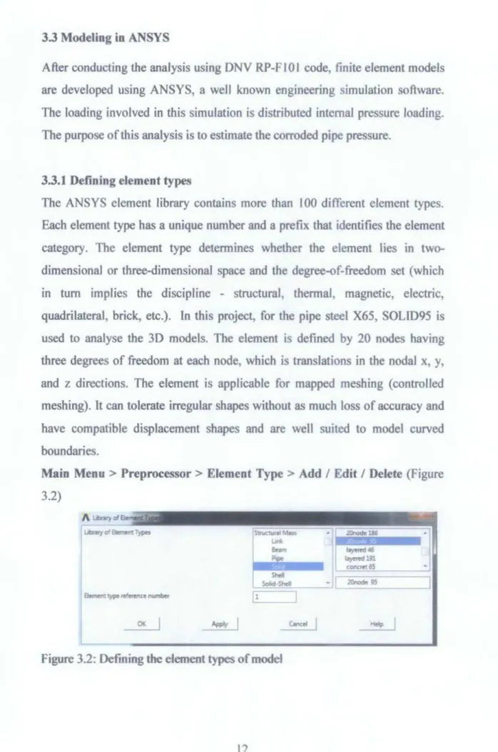
3.3 Modeling in ANSYS

After conducting the analysis using DNV RP-F I 0 I code, finite element models are developed using ANSYS, a well known engineering simulation software. The loading involved in this simulation is distributed internal pressure loading. The purpose of this analysis is to estimate the corroded pipe pressure.

3.3.1 Defining element types

The ANSYS element library contains more than 1 00 different element types. Each element type has a unique number and a prefix that identifies the element category. The element type determines whether the element lies in two-dimensional or three-two-dimensional space and the degree-of-freedom set (which

in turn implies the discipline - structural, thermal, magnetic, electric, quadrilateral, brick, etc.). In this project, for the pipe steel X65, SOLID95 is used to analyse the 3D models. The element is defined by 20 nodes having three degrees of freedom at each node, which is translations in the nodal x, y, and z directions. The element

is

applicable for mapped meshing (controlled meshing). It can tolerate irregular shapes without as much loss of accuracy and have compatible displacement shapes and are well suited to model curved boundaries.

Main Menu> Preprocessor> Element Type> Add I Edit I Delete (Figure

3.2)

()I(

I

_{Apply '}

Figure 3.2: Defining the element types of model

1~46 ~191

CHAPTER4

RESULTS AND DISCUSSIONS

4.1 DNV Code Results

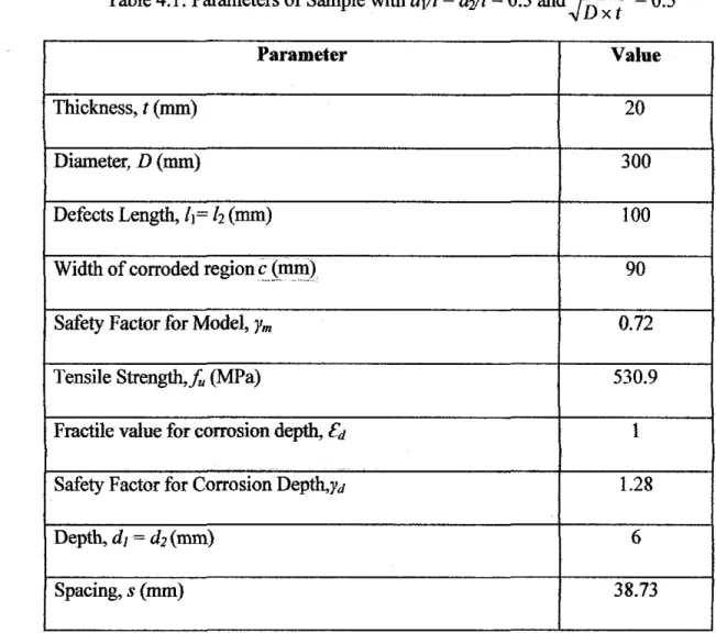
The calculation is based on assessment of interacting defects (Calibrated safety factor, Part A). The parameters of pipe steel X65 that

will

be used in the calculation is stated as in Table 4.1.

s

Table 4.1: Parameters of Sample with d/t

=

dz/t

=

0.3 and

.J

Dx t

=

0.5

Parameter Value

Thickness, t (mm) 20

Diameter, D (mm) 300

Defects Length, /1- /2 (mm) 100

Width of corroded region

c.Jffilll)

90

Safety Factor for Model, Ym 0.72

Tensile Strength,.fu (MPa) 530.9

Fractile value for corrosion depth,

Ed

1

Safety Factor for Corrosion Depth,yd 1.28

Depth, d1 = d2(mm) 6

4.1.1 Allowable Corroded Pressure for Single Defects, PI and

P2

1. Length Correction Factor,

Q1

Qt= = ( ) 2 1+0.31 100mm .,/300mm x 20mm = 1.231

2. Allowable corroded pressure, PI and P2

2tfu(1-

YtJ(dt!t)*)

pt,pz

=

')1n

(D-t)(l

p(d~t)*)

= 0. 72x2x20x530.9x(l-1.28(0.38)) (300-20)(1 1.28(0.38)) 1.231 = 46.37MPa

4.1.2 Allowable Corroded Pressure for Interacting Defects, Pnm

l. Total length, lnm i=m-J. /nrn

=

fm

+

~)/;

+

Si)

i=n = (100+ 100 + 38.73) mm =238.73mm

2. Effective Depth,

dnm

i=m

l:.d;/;

dnm

=

_,__i=.:.:..n -[nm

=

(6mmx 100mm}+(6mmx 100mm} 238.73mm =5.027mm

3. Length Correction Factor,

Qnm

1+0.31(

1

nm ) 2

--rn;

~--~---~2

I+0.3l(

238.73mm ) = .J300mmx 20mm =

1.986

4. Adjusted depth ratio, (d,../t)* (dnm /t)*=(dnm lt)meas

= (5.027)

20.00 = 0.251

5.

Allowable corroded pressure,Pnm

=

0. 72x2x20.00x530.9x(l-1.28(0.251))

(300-20{1 1.28(0.251))

1.986

=

44.199MPa

4.1.3 Maximum Allowable Corroded Pressure,pc""

P = min (p J, Pnm)

4.2 Overall Result Summary

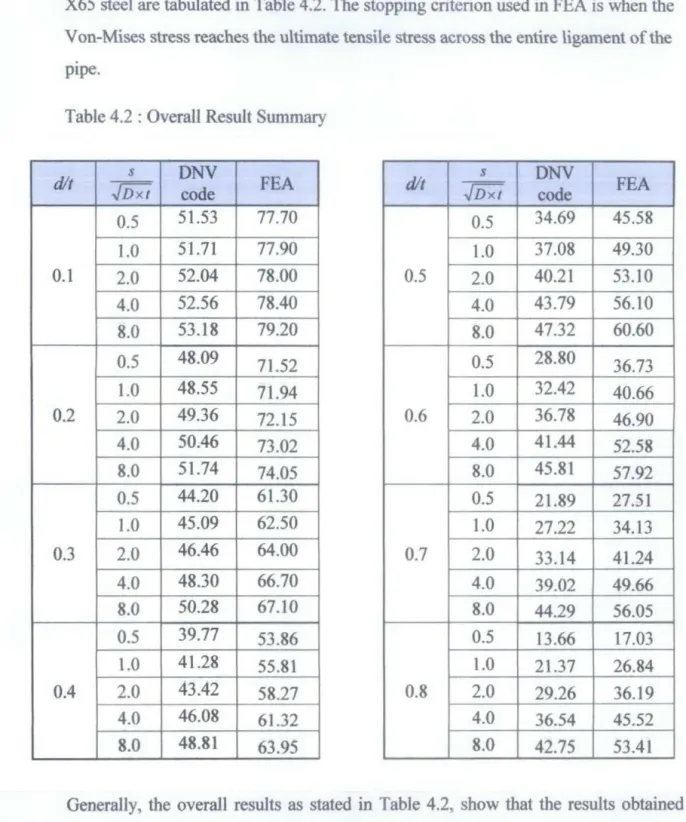
The overall results summary of empirical solution and FEA non-linear analysis for X65 steel are tabulated in Table 4.2. The stopping criterion used in FEA is when the Von-Mises stress reaches the ultimate tensile stress across the entire ligament of the plpe.

Table 4.2 : Overall Result Summary

dlt s DNV .JDxt code FEA dlt s DNV .JDxt code FEA 0.5 51.53 77.70 0.5 34.69 45.58 1.0 51.71 77.90 1.0 37.08 49.30 0.1 2.0 52.04 78.00 0.5 2.0 40.21 53.10 4.0 52.56 78.40 4.0 43.79 56.10 8.0 53.18 79.20 _8.0 47.32 60.60 0.5 48.09 _71.52 0.5 28.80 _36.73 1.0 48.55 _{71.94 1.0} 32.42 _40.66 0.2 2.0 49.36 _72.15 0.6 2.0 36.78 _46.90 4.0 50.46 _73.02 4.0 41.44 52.58 8.0 51.74 74.05 8.0 45.81 57.92 0.5 44.20 61.30 0.5 21.89 27.51 1.0 45.09 62.50 1.0 27.22 34.13 0.3 2.0 46.46 64.00 0.7 2.0 _{33.14 41.24} 4.0 48.30 66.70 4.0 39.02 49.66 8.0 50.28 67.10 8.0 44.29 56.05 0.5 39.77 53.86 0.5 13.66 17.03 1.0 41.28 _55.81 1.0 21.37 26.84 0.4 2.0 43.42 _58.27 0.8 2.0 29.26 36.19 4.0 46.08 61.32 4.0 36.54 45.52 8.0 48.81 63.95 8.0 42.75 53.41

Generally, the overall results as stated in Table 4.2, show that the results obtained from FEA is higher compared to the values obtained using DNV Code. The non linear analysis yield results which are in similar trend with the empirical solution obtained from the DNV Code.

-~ 1.000 0.900 _....

_....

..

0800 ~DNV <0 _code (1. ~ 0.700 i _0.600 ~ _F[A D.

• •

•

•

•

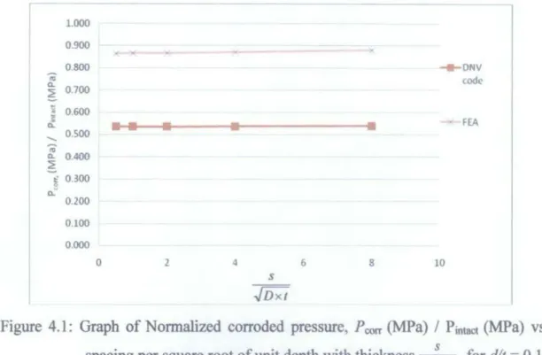
... 0.500 <0 (1. ~ 0.400 g 0.300 (1.~ 0.200 0.100 0.000 0 2 4 6 8 10 s ../Dxt

Figure

4.1:

Graph of Normalized corroded pressure,

Poorr

(MPa) I Pintact (MPa) vs

spacing per square root of unit depth with thickness,

~

, for dlt = 0.1

-vDxt

Figure

4.1

shows the comparison between the results from

DNV

Code and

FEA

for

case d/t = 0.1. The graph shows that the effect of spacing between the defects does

not differ much toward the failure pressure for both techniques .. In other word, the

effect of interaction for defects with depth of l 00/o of pipe wall thickness will not

have significant impact toward the pipe failure pressure. The Ratio of

FEA

over

DNV Code is 1.499. 0.900 0.800 <0 0.700 (1. ~ -: 0.600 :(

~

-~--~----~---

--

--·

t1. 0.500 • • • • ~ 0.400 "' (1. ~ 0.300

"

D.e 0.200 0.100 0000 0 2 4 s ../Dxt 6 8 ~ ONV code .. F[A 10

Figure 42: Grnph of Nonnalized oomxted presswe, P OCYrr (MPa) I Pnrtact (MPa) vs

spacing per square root of unit depth with thickness,

~,for

d/t

=

0.2

Figure 4.2 shows the comparison between the results from DNV Code and FEA for case

d/t

=

0.2. As the distance between the defects increase the failure pressure increase slightJy. The interaction start to occur when the distance between the defects is small. However, for defect with depth of 20% of pipe wall thickness, it only experienced small interaction effect. Thus the failure pressure only has minor increment as the distance of the defects is increased. The ratio of FEA over DNV Code is 1.462. 0.800 0700 ..., ,--=1".: ~ - - -ONV Q. _{0.600 Cod('} ~ ~ 0500

•

•

a

...

•

_{.,... F(A} tl. ... 0400 ~ Q. _0.300 ~ ~ 0.200 Q.y 0.100 0000 0 2 4 6 8 10 s .JDxt

Figure 4.3: Graph of Normalized corroded pressure, Pcorr (MPa) f Pintact (MPa) vs spacing per square root of unit depth with thickness,

~

, for d/t = 0.3

-vDxt

Figure 4.3 shows failure pressure comparison for case d/t = 0.3. The graph shows that the failure pressure is lower when the distance between defects is small and as

s

the distance between the defects increase up to ..[jj;t 4 the failure pressure increase significantJy. For

.J~

x

t

> 4, the failure pressure increase with small amount. The effect of interaction is significant when the distance is small and later the effect of interaction is small as spacing between defects is far from each other. Defects with

depth of 30% of pipe wall thickness will show significant interaction effect when the distance between defects is small,

~

< 4. The ratio of FEA over DNV Code is

-vDxt 1.373.

I

0.800 0.700 ~

..

-

ONV Q.. _0.600 ~ _code ~ ~ 0.500

•

s

•

Q.

...---

...

F(A ... 0.400 ~ Q.. _0.300 ~ ~ 0 200 Q.. 0.100 0000 0 2 4 6 8 10 s .JDxt

Figure

4.4:

Graph of Normalized corroded pressure, P corr (MPa) I

Pmtact

(MPa) vs spacing per square root of unit depth with thickness, ~, for d/t =

0.4

"1/Dxt

Figure

4.4

shows failure pressure comparison for case

dlt

=

0.4

.

The graph shows that the initial failure pressure is lower and as the distance between the defects increases the failure pressure increase. For defects with depth of

40%

of pipe wall thickness, the interaction effect is high when the distance between defects is small and the effect gradually decreases as the distance is increased, resulting increased failure pressure. The ratio ofFEA over

DNV

Code is

1.

338.

0800 0.700 ~ Q.. ~ 0.600 §

"

0.500 0.. ... _0.400 to Q.. _0.300 ~ ~ 0.200 n. 0.100 0.000 0 2 4 s .JDxt 6 8 10 ONV code f(A

Figure 4.5: Graph of Normalized corroded pressure,

P

oorr (MPa)

I

Pintact (MPa) vs

Figure 4.5 shows failure pressure comparison for case d/t == 0.5. The graph shows that the initial failure pressure is lower and as the distance between the defects increases, the failure pressure increase. For defects with depth of 50% of pipe wall

thickness, the interaction effect show similar pattern as for case d/t

=

0.4 but the effect of interaction is increased. The difference in term of failure pressure is high between the small defects spacing and large defects spacing. The ratio of FEA over

DNV Code is 1.305. 0.700 0.600 -;;; 0.. ~ 0.500 ~ i _0.400 0.. ... -;;; 0.300 0.. ~

i

0.200 "' 0..~ 0.100 0000 0 2 4 s .JDxl 6 8 ~DNV code FEA 10

Figure 4.6: Graph of Normalized corroded pressure.

Pcorr

(MPa)

I

Pmtact (MPa) vs spacing per square root of unit depth with thickness, ~.for d/t

=

0.6

-vDxl

Figure 4.6 shows failure pressure comparison for case dlt

=

0.6. The graph shows that failure pressure increase significantly as the distance between defects increased. For defects with depth of 60% of pipe wall thickness, the interaction effect is greater at small defects spacing resulting low failure pressure. Similar trend as from the previous case, the failure pressure increase as the distance between defects increased. The ratio ofFEA over DNV Code is 1.267.

0.700 0600 "'

i

0.500 i 0.400 n. ... "' 0.300 0.. ~ ~ 0.200 Q. 0.100 0.000 0 2 4 6 8 ~DNV code -... FEA 10

Figure 4.7: Graph of Normalized corroded pressure,

Pwrr

(MPa)

I Pmtact

(MPa) vs spacing per square root of unit depth with thickness, ~ for d/t

=

0. 7

..;Dxt

Figure 4. 7 shows failure pressure comparison for case d/t = 0. 7. The graph shows that failure pressure increase significantly as the distance between defects increased. For small defects spacing, the FEA result has small difference compared to the value DNV Code. But as the distance between defects increase, the difference between DNV Code and FEA is higher. For defects with depth of 70% of pipe wall thickness,

the interaction effect is greater at small defects spacing resulting low failure pressure. The failure pressure increase drastically as the distance between defects increased. The ratio ofFEA over DNV Code is 1.259.

-~ 0.700 0.600 ;.· DNV Iii _code 0.. 0.500

-2 .;' :;

....

i 0.400

;7

FEA "-... Iii _0.. 0300 2 ~ 0.200 o..u 0.100 0.000 0 2 4 6 8 10 s ..JDxt

Figure 4.8: Graph of Normalized corroded pressure, P corr (MPa) I

Pmtact

(MPa) vs

Figure 4.8 shows failure pressure comparison for case d/t

=

0.8. The graph shows that failure pressure increase significantly as the distance between defects increased. For small defects spacing, the FEA result is approaching the DNV Code. The difference of failure pressure between DNV Code and FEA is small when the defect spacing is small. And as the distance increase, the failure pressure increase. For defects with depth of 80% of pipe wall thickness, the interaction effect is greater at small defects spacing resulting low failure pressure. For small defects spacing, even though the results yield from both method show nearly similar results but only with small difference, the value from FEA method is higher compared to DNV Code. The failure pressure increase drastically as the distance between defects increased. The ratio ofFEA over DNV Code is 1.247.

- - - -

-1.00 0.90 - 0.80 111 Q. ~0.70 i0.60

••

•

•

•

-+-d/t·O.l

•

_~

- . -d/t 0.2 -+-d/t 0.3

~

- d / t•0.4 Q. ..._0.50 - d/t•O.S

-

~ 0.40 - . -d/t·0.6 ~ -d/t~o.7 'iOJO ... - d/t•0.8 a."o1o 0.10 0.00 0 2 4 6 8 10

Figure 4.9: Graph of Normalized corroded pressure,

Pcorr

(MPa)

I Pm

tact (MPa) vs

spacing per square root of unit depth with thickness, ~, for the FEA

vDxt

result.

From the graph above, it is observed that as the distance between defects increase,

the maximum allowable corroded pressure will increase. For defect with smaller depth, the failure pressure has no significant changes as the distance between defects increased. Meanwhile, defect with greater depth will result on large failure pressure

Furthermore, as the depth of the defects increase, the failure pressure will decrease. The failure pressure at the small defects spacing reduced significantly and the effect of interaction is critical within this region. This shows that, when the spacing

between the defects is small, they start to interact with each other and reduced the maximum allowable corroded pipe pressure.

1.60 1.40 Ill

-=

¢ _1.20 1..1 ;....

~

1.00 V 0.481xL 0.805x t 1.583 • ,wg ~ 0.80 n1.1X r-1 r-. - mtn

....

0.60 ¢ C> : 0.40 eo: -Poly (clvg) Q:; 0.20 0.00 0.00 0.20 0.40 0.60 0.80 1.00 d/t

Figure 4.10: Graph of Ratio ofFEA over DNV Code vs depth per unit thickness. The result from FEA is always higher than

DNV

Code. This is due to safety factor applied in the empirical calculation which yields on lower corroded pipe failure

pressure as to avoid reaching the exact failure pressure during standard operating condition. Figure 4.10 shows the factor of the ratio between FEA and DNV Code.

The factor is not a fixed value since the multiplication factor is not the same for

every cases of defects depth. This is due to stress concentration at the edges of the

defects during the simulation process. The deeper the defect depth, the higher stress concentration occur at the edge of the defect. Since the remaining pipe wall thickness

reduced, the stress distribution on the entire ligament of the edge easily reaches the

failure criterion. From the graph above, it shows a decreasing trend as the depth of

the defects is increasing. The best plot on the graph is

based

on the average value of

the ratio of FEA over

DNV

Code. The factor can be expressed as a function of:

Figure 4.11: Element solution of Von Misses stress distribution for d/t

=

0.2,

s

.JDxt = 0.5 (Internal view)

Figure 4.12: Element solution of Von Misses stress distribution for d/t = 0.2, s

edge

Figure 4.11 and 4.12 show the element solution of the model for d/t

=

0.2 and

s

..rn;:1

0.5. The stopping criterion of the simulation is when the Von Misses stress

distribution reaches the ultimate tensile strength (crUTs = 530.9MPa) across the entire

thickness of the ligament.

Point of

Figure 4.13: Closed view on the defect area for d/t

=

0.2 and ~

=

0.5.

-vDxt

As the pressure applied on the internal surface of the pipe increased, the critical stress start to propagate along the edge of the defect and spread around the defect area. The assessment of the entire ligament is determined by consider the stress

distribution across the thickness on several points at the critically defect area. Figure 4.13 shows the maximum stress point (MX) which occur at the edge of the defect. The stress distribution is analysed based on three points along the line of critical edge; the maximum stress point, middle point, and end point of the edge.

CHAPTERS

CONCLUSION AND RECOMMNEDATION

5.1 CONCLUSION

Consideration for maintenance or replacement of corroded pipeline is crucial beeause it affects directly to the cost of the

firm.

The available codes that are widely being used in the industry is too conservative. This may lead to unnecessary maintenance or premature replacement of corroded pipeline. Therefore, the FEA is one of the accurate methods to assess the burst strength of the corroded pipeline. Burst strength of pipeline with interacting corrosion defects can be accurately predicted by FEA using ANSYS software. The application of FEA can reduce the conservatism involved in the conventional methods. From this study, the ratio of FEA over DNV Code is a function of (d/t) given by: Factor = 0.48l(d/lj2 -0.805(dll) + 1.583.

5.2 RECOMMENDATION,

Distance between defects is one of major factor toward the interaction to be occurred between defects. As the distance of the defect is increasing, the effect of interaction decrease and lead to increase in maximum allowable pipe failure pressure. In this study, it only sees the effect of interacting defects with similar defect depth. Further study can focus on the effect of interaction between defects with different depth.

REFERENCES

[I] N. Shafiq, M.C. Ismail, Belachew C. T., K.Saravanan, and M.F. Nuruddin, 2010. Burst Test, Finite Element Analysis and Structural Integrity of Pipeline System. Hydrocarbon Asia's Engineering and Operations Convention, Kuala Lumpur, Malaysia.

[2] B.A Chouchaoui and R.J Pick, 1996. Behavior of Longitudinal Aligned Corrosion Pits, Int J. Press. Ves. & Piping, 67: .17-35.

[3] DNV, Oct 2004. Recommended Practice DNV-RP-FIOI, Corroded Pipeline, Hovik, Norway. Pp42.

[4] T.A Netto, U.S. Ferraz, S.F Estefen, 2005. The Effect of Corrosion Defects on The Burst Pressure of Pipelines. Journal of construction steel research, 61:

1185-1204.

[ 5] Belachew C. T ., M. C. Ismail, and K.Saravanan, 2011. Burst Strength Analysis of Corroded Pipelines by Finite Element Method, Journal of Applied sciences. Asian Network for Scientific Information.

[6] M. G. Fontana, 1987. Corrosion Engineering. Third Edition, Me Graw-Hill, London. ISBN- 0-07-100360-6, p: 4.

[7] Pipeline Corrosion, Public Affairs - White papers, Nace International

Retrieved from

http://www .nace.org/content.cfm?parentid= I 046&currentiD= 1424

[8J ANSIJASME, 1991. Manual for Determining the Remaining Strength of Corroded pipelines: A supplement to ASME B31 Code for Pressure Piping. American Society of Mechanical Engineers, USA., pp 55.

{9] R.C.C. Silva, J.N.C. Guerriro, A.F.D. Loula, 2007. A Study of Pipe Interacting Corrosion Defects using FEM and Neural networks, Advance in Engineering Software, 38: 868-875.

[10] J.F. Kiefner and P.H. Vieth, 1989. A Modified Criterion for Evaluating the Remaining Strength of Corroded Pipe. Final report on Project PR 3-805, Pipeline Research Committee, American Gas Association.

[II] Belachew, C.T., M.C. Ismail, and K.Saravanan, 2009. Capacity assessment of corroded pipelines using available codes. NACE Asia Pacific, Kuala Lumpur. Retrieved from http:/leprints.utp.edu.my/1772/1/NACE _Conference _Paper.pdf

[12] Y.K.Lee, Y.P. Lim, M.-W.Moon, W.H. Bang. K.H. Oh, W.-S. Kim, 2005. The prediction of failure pressure of gas pipeline with multi corroded region, Material Science Forum, Vol475-479, p 3323-3326.