bayesvl: Visually Learning the Graphical Structure of Bayesian Networks and Performing MCMC with 'Stan'

(1)

1

bayesvl: Visually Learning the Graphical

Structure of Bayesian Networks and

Performing MCMC with 'Stan'

Quan-Hoang Vuong (1,2)

Email: [email protected] Viet-Phuong La (1,2)

Email: [email protected]

(1)_{AISDL, Vuong & Associates} (2)

SDAG, Centre for Interdisciplinary Social Research, Phenikaa University

5/25/2019 11:19:34 AM

Version: Officially published on CRAN May 24, 2019 Hanoi, Vietnam

Suggested Citation:

La, V.P, & Vuong, Q.H. (2019). bayesvl: Visually Learning the Graphical Structure of Bayesian Networks and Performing MCMC with 'Stan'. The Comprehensive R Archive Network (CRAN): <https://cran.r-project.org/package=bayesvl>; version 0.8.5 (May 24, 2019).

(2)

2

*Important note:

This User Guide is written following the logic that aims to enable users to acquire Bayesian computation skills through examples using real data. Therefore, users are advised to perform MCMC computations very early on by repeating the R code provided in the file simulation_example.R deposited at:

https://github.com/sshpa/bayesvl/blob/master/References/simulation_example.R. The performing of the MCMC computing code given in the file will require users' computers to meet technical requirements and to follow the algorithmic logic. Also, a critical component apart from installing bayesvl itself is rstan, which can be accessed and downloaded from here:

https://github.com/stan-dev/rstan/wiki/RStan-Getting-Started. Users are strongly advised to install relevant packages for successfully performing the MCMC problem, as specified in the notes contained in our example file.

Introduction to the BayesVL Project

“BayesVL” is a long-term project for developing a computer program run on the programming language R. This statistics program focuses on building an application algorithm for Markov Chain Monte Carlo (MCMC) simulation, which is then wrapped up in an “R package” called bayesvl [1].

The project and programs under development, as well as the user guide, including reference materials, can be accessed openly at Github

<https://github.com/sshpa/bayesvl> [2].

The development of the bayesvl package, following a worldwide trend and growing popularity of the R language as a powerful statistical programming environment, started in late 2017 [3,4]. At the A.I. for Social Data Lab (AISDL), we also focus on improving our research process and aim to solve the problems posed by frequentist statistics, such as the plausibility of results, the reproducibility crisis, and the

controversy related to interpreting the “p-value” [5,6]. Moreover, it comes to our attention that the ability of R to generate graphics, coupled with simulated data using Markov Chain Monte Carlo (MCMC) method, whether on Stan or JAGS, can make a powerful tool in diagnosing and presenting research results [7].

Mathematical foundation

Bayes’ Theorem for conditional probability distribution:

𝑓(𝜃|𝑑𝑎𝑡𝑎) = 𝑓(𝑑𝑎𝑡𝑎|𝜃) × 𝑓(𝜃) 𝑓(𝑑𝑎𝑡𝑎)

(3)

3

Here, 𝑓(𝜃|𝑑𝑎𝑡𝑎)is the posterior distribution for a parameter 𝜃, 𝑓(𝑑𝑎𝑡𝑎|𝜃)is the sampling density of the data, 𝑓(𝜃)is the prior distribution for the parameter 𝜃, 𝑓(𝑑𝑎𝑡𝑎) is the marginal probability of the data. As the sample density is proportional to the likelihood function, we can rewrite the Bayes’ Theorem as follow:

𝑝(𝜃|𝑑𝑎𝑡𝑎)∝ 𝑝(𝑑𝑎𝑡𝑎|𝜃) × 𝑝(𝜃)

posterior ∝ likelihood ×prior

The objective of Bayesian statistics is to represent the uncertainty of a model's parameters through a prior probability distribution; then with new data, we can update this probability distribution and arrive at the posterior distribution, in which the uncertainty is reduced.

From a Bayesian perspective, we start with a prior probability of an event, then update the credibility of the event to have a posterior probability. Whenever new data are gathered, this posterior becomes a new prior for the next computation. In fact, this process is very similar to how scientists do science.

In any research study, data are gathered to evaluate a specific scientific hypothesis. Rarely do we start this investigation with complete ignorance, instead it is usually the case that previous studies have provided a priori information to start this belief-updating process.

The current stage of bayesvl v0.8

At the moment bayesvl is marked version 0.8, the program contains approximately 3000 lines of code. Before version 0.8, a part of the code has been employed for a number of our research studies [8-11].

bayesvl v0.8 has included a user guide in both Vietnamese and English, and the program, itself, can be deployed for a variety of statistics problems.

User guide for bayesvl R Package: An application-driven

approach

(4)

4

a. Focusing on the application of bayesvl, rather than repeating the mathematical formalism behind the MCMC method, has become the standard for Bayesian statistics textbooks.

b. Using a real problem with a real dataset, and real results to demonstrate the logic of problem identification, model construction, execution, simulation, and result interpretation.

c. The codes are put into relevant sections to highlight their function and to bridge between theory and practice.

Problem No.1

Problem No. 1 uses the dataset titled “20180224_Legends_345.csv” [22]. This is a dataset that has encoded Vietnamese folktales by attributes related to their content, which enables statistical analyses of the tales on a systematic basis. A study using Bayesian analysis to uncover behavioral patterns in the tales was published in December 2018 [8].

Problem No. 1 will analyze outcome associated with behaviors of lying and violence of the main characters in the folktales and evaluate the association of the Three Teachings (Buddhism, Confucianism, and Taoism) with said behaviors.

Below is a simple model for the research problem:

Out ~ VB + VC + VT + Lie + Viol + (Int1 + Int2)

Installing bayesvl R Package

The bayesvl package can be installed directly in R from the following Github address <https://github.com/sshpa/bayesvl> using the following basic commands:

> install.packages("devtools")

> devtools::install_github("sshpa/bayesvl") Calling out package BayesVL

> library("bayesvl")

If users need to also install the rstan package separately, check out rstan Github:

https://github.com/stan-dev/rstan/wiki/RStan-Getting-Started. The rstan package appears to perform well with R 3.5.1 or newer.

(5)

5

Dataset and estimations

The first step is to enter the dataset into the application program bayesvl. A dataset serves two primary functions:

a) Problem identification; b) Simulation to find results. Data and model construction

First, we need to call out the dataset “Legends345”, which is provided in the package

bayesvl, using the following R commands:

data(Legends345) data1 <- Legends345 head(data1)

The variables:

• Lie: whether the main character lies

• Viol: whether the main character employs violence

• VB: whether the main characters' behaviors express the value of Buddhism

• VC: whether the main characters' behaviors reflect the value of Confucianism

• VT: whether the main characters' behaviors express the value of Taoism

• Int1: Whether there are interventions from the supernatural world

• Int2: Whether there are interventions from the human world

• Out: Whether the outcome of a story is favorable for its main characters These are the observational data, which were directly collected through reading and encoding these elements into a data table.

A complete description of the dataset “Legends345” can be viewed using R’s command for help:

help(Legends345)

A data help page will be shown with explanations and usage of the dataset and data variables.

Model

The purpose of the model is to evaluate the influence of the Three Teachings (“VB”, “VC”, “VT”) on lying (“Lie”) and violent behavior (“Viol”) of the main characters in

(6)

6

the folktales. This influence is evaluated based on whether the outcome of the stories is good or bad for the main character.

Specifically, we are interested in finding out whether the main character lied or committed violent acts and at the same time, and their behaviors express certain core values of the Three Teachings; for example, the main character lies but still succeeds.

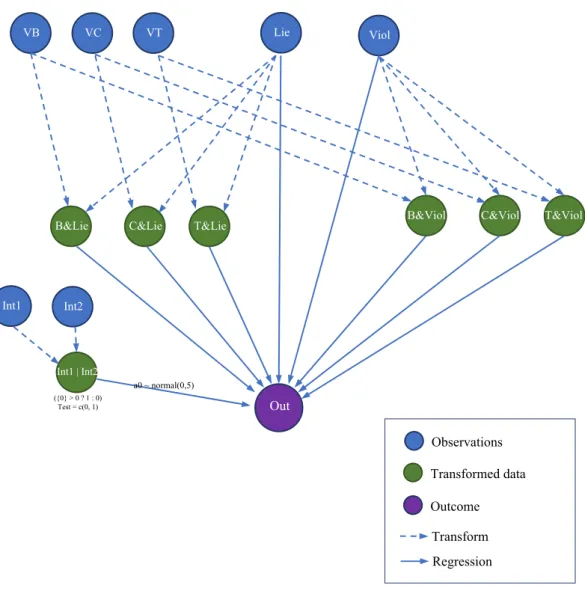
The preliminary model, designed based on these expectations, is visually presented in Figure 1.

Hình 1

Figure 1 is a logic map of the causal relationship between different levels of variables and the outcome ("Out").

Model interpretation:

The model is a multi-level varying intercept model. The following is the most basic form of a multi-level varying intercept linear regression model.

Lie

Out

VB VC VT Viol

B&Lie C&Lie T&Lie B&Viol C&Viol T&Viol

Observations Transformed data Outcome Transform Regression Int1 Int2 Int1 | Int2 a0 ~ normal(0,5) ({0} > 0 ? 1 : 0) Test = c(0, 1)

(7)

7

𝑦 = 𝛼 + 𝛽𝑥 + 𝜖

Using bayesvl, we can create the model and load the observation data:

# Design the model model <- bayesvl()

model <- bvl_addNode(model, "O", "binom") model <- bvl_addNode(model, "Lie", "binom") model <- bvl_addNode(model, "Viol", "binom") model <- bvl_addNode(model, "VB", "binom") model <- bvl_addNode(model, "VC", "binom") model <- bvl_addNode(model, "VT", "binom") model <- bvl_addNode(model, "Int1", "binom") model <- bvl_addNode(model, "Int2", "binom")

The function bvl_addNode(model, "O", "binom") and other similar ones are new functions that are written just for bayesvl. The function bvl_addNode can be used to add new nodes to a model. This function includes the following arguments:

• dag: or model in the example above. This argument is the target for adding nodes. Dag is called out from the first line of code when we start a model: model <- bayesvl().

• name: or "O" in the example above; this argument gives a name for a node in a model.

• dist: in the example above, dist defines the distribution for each node, including two types of statistical distribution: normal (or standard

distribution) and binomial. These two types of distribution are coded into "norm" or "binom". When we combine two variables, we have a new distribution called "trans" or transform.

In general, with the function above bvl_addNode(model, "O", "binom"), a new node is added to the model, this node is named “O”, and is binomially distributed. The mathematical formula to compute the probability distribution of the binomially distributed variable 𝑥:

𝑝𝑟(𝑥|𝑛, 𝑝) = 𝑛

𝑥 𝑝 (1 − 𝑝)

In which, 𝑛 is the total number of trials, 𝑝 is the probability of 𝑥 successes throughout the trials.

(8)

8

A complete guide of creating a network model in bayesvl can be found in R using the commonly used command help:

help("bayesvl graphs")

In the model in Figure 1, the variables “O”, “Lie”, “Viol”,… are all binomially distributed. In Figure 1, they are presented by blue nodes .

To evaluate the influence of the Three Teachings (“VB”, “VC”, “VT”) and lying (“Lie”) on the outcome of the stories, we join the Three Teachings variables with the lying variable to create transformed data (in Figure 1, the transformed data are

represented as green nodes ):

• B_and_Lie: the main character behaves following the core values of

Buddhism, yet there are details/contents in the story showing this character lies.

• C_and_Lie: the main character behaves following the core values of Confucianism, yet there are details/contents in the story showing this character lies.

• T_and_Lie: the main character behaves following the core values of

Buddhism, yet there are details/contents in the story showing this character lies.

To evaluate the influence of the Three Teachings (“VB”, “VC”, “VT”) and violent behavior (“Lie”) on the outcome of the stories, we join the Three Teachings variables with the violent variable to create transformed data:

• B_and_Viol: the main character behaves following the core values of Buddhism yet commits violent acts.

• C_and_Viol: the main character behaves following the core values of Confucianism yet commits violent acts.

• T_and_Viol: the main character behaves following the core values of Confucianism yet commits violent acts.

In terms of mathematical formalism, we can express these relations using the mathematical operator (*) between the two variables:

B_and_Lie = B * Lie C_and_Lie = C * Lie T_and_Lie = T * Lie B_and_Viol = B * Viol C_and_Viol = C * Viol T_and_Viol = T * Viol

(9)

9

The relation for transformed data is represented in Figure 1 using the dash-line arrow ( ).

We can generate the transformed data nodes using bayesvl in R:

model <- bvl_addNode(model, "B_and_Viol", "trans") model <- bvl_addNode(model, "C_and_Viol", "trans") model <- bvl_addNode(model, "T_and_Viol", "trans")

To define the transformed data such as "B_and_Viol" from the observation data such as "VB" and "Viol", using the mathematical operator (*):

model <- bvl_addArc(model, "VB", "B_and_Viol", "*") model <- bvl_addArc(model, "Viol", "B_and_Viol", "*") model <- bvl_addArc(model, "VC", "C_and_Viol", "*") model <- bvl_addArc(model, "Viol", "C_and_Viol", "*") model <- bvl_addArc(model, "VT", "T_and_Viol", "*") model <- bvl_addArc(model, "Viol", "T_and_Viol", "*")

Similar to bvl_addNode, bvl_addArc is a function written for bayesvl to add new arcs between two nodes in a model. For example, bvl_addArc(model, "VB", "B_and_Viol", "*")has the following arguments:

• dag: or model in the example above. This is a target to add nodes. Dag is called out from the first line of code when we start a model: model <- bayesvl().

• from and to: or "VB" and "B_and_Viol" in the model. This represents which pair of nodes we want to generate an arc for and its direction.

• Mathematical operator "*" defines the transforming data relationship between the two nodes. In other cases, such as regression relationship, the relationship between two nodes can have forms such as "varint" or "slope".

To evaluate whether the outcome of a story is changed because of intervention either from the supernatural or human force, we combine the two observation variables "Int1" and "Int2" into one new transformed variable:

• Int1_or_Int2: there exists an intervention in a story of either the supernatural or the humans in the stories.

(10)

10

Specifically, the intervention of the supernatural (“Int1”) can come from characters such as the Bodhisattva or the Buddha, or the fairy. The intervention of human (“Int2”) comes from the people such as the King, the mandarine, or the landlords. In terms of mathematical formalism, we have:

Int1_or_Int2 = (Int1 + Int2 > 0 ? 1 : 0)

As such, when the new variable is the sum of two observation data “Int1” and “Int2,” if this sum is greater than 0, it means at least 1 in two observation data takes the value of one (there is intervention). In this case, the value of the transformed data will be 1. If the sum is equal to 0, the transformed data take on value 0.

As such, we have one variable to represent the intervention of either supernatural force (fairy, Buddha, etc.) or human force (king, mandarin, etc.).

The code for constructing the new variables using bayesvl:

model <- bvl_addNode(model, "Int1_or_Int2", "trans", fun = "({0} > 0 ? 1 : 0)", out_type = "int", lower = 0, test = c(0, 1))

Because the transformed data "Int1_or_Int2" we are aiming to create is more complicated compared to other variables, the function bvl_addNode, in this case, has a more complicated line of codes as more arguments are included. Besides the similar arguments such as model, model, "Int1_or_Int2" and "trans", we have:

• fun: is the procedure to change node. The condition of fun is based on the mathematical foundation of "Int1_or_Int2" we have presented above.

• out_type: represents the format of output int (integer) or real (real numbers).

Defining the new variable “Int1_or_Int2” from the observation data (“Int1” và “Int2”) through the mathematical operator (+):

model <- bvl_addArc(model, "Int1", "Int1_or_Int2", "+") model <- bvl_addArc(model, "Int2", "Int1_or_Int2", "+")

To find out the correlations of the outcome of the stories (“O”), we run a regression of the variables defined above with the observation data “O”. We need to define the regression relationship among the nodes; therefore, in the function bvl_addArc, the nodes have a varying slope relation ("slope").

(11)

11

We construct the regression relationship between the transformed data that have the lying element and the outcome variable (“O”):

model <- bvl_addArc(model, "B_and_Lie", "O", "slope") model <- bvl_addArc(model, "C_and_Lie", "O", "slope") model <- bvl_addArc(model, "T_and_Lie", "O", "slope") model <- bvl_addArc(model, "Lie", "O", "slope")

We construct the regression relationship between the transformed data that have the violent element and the outcome variable (“O”):

model <- bvl_addArc(model, "B_and_Viol", "O", "slope") model <- bvl_addArc(model, "C_and_Viol", "O", "slope") model <- bvl_addArc(model, "T_and_Viol", "O", "slope") model <- bvl_addArc(model, "Viol", "O", "slope")

This is a varying slope regression, in which the intercepts determine the position of the linear regression line according to the y-axis of the outcome variable, the slope coefficient defines the angle of the line. As such, when the intercepts vary, we have the linear model with the following forms:

We construct the varying intercepts regression for the variable "Int1_or_Int2". As a result, we can evaluate the outcome of the story in two cases: (1) with

intervention, and (2) without intervention.

model <- bvl_addArc(model, "Int1_or_Int2", "O", "varint", priors = c("a0_ ~ normal(0,5)", "sigma_ ~ normal(0,5)"))

(12)

12

Overall, to generate all the mathematical model for the network of nodes in Figure 1 using bayesvl in R:

# Design the model model <- bayesvl()

model <- bvl_addNode(model, "O", "binom") model <- bvl_addNode(model, "Lie", "binom") model <- bvl_addNode(model, "Viol", "binom") model <- bvl_addNode(model, "VB", "binom") model <- bvl_addNode(model, "VC", "binom") model <- bvl_addNode(model, "VT", "binom") model <- bvl_addNode(model, "Int1", "binom") model <- bvl_addNode(model, "Int2", "binom") model <- bvl_addNode(model, "B_and_Viol", "trans") model <- bvl_addNode(model, "C_and_Viol", "trans") model <- bvl_addNode(model, "T_and_Viol", "trans") model <- bvl_addArc(model, "VB", "B_and_Viol", "*") model <- bvl_addArc(model, "Viol", "B_and_Viol", "*") model <- bvl_addArc(model, "VC", "C_and_Viol", "*") model <- bvl_addArc(model, "Viol", "C_and_Viol", "*") model <- bvl_addArc(model, "VT", "T_and_Viol", "*") model <- bvl_addArc(model, "Viol", "T_and_Viol", "*") model <- bvl_addArc(model, "B_and_Viol", "O", "slope") model <- bvl_addArc(model, "C_and_Viol", "O", "slope") model <- bvl_addArc(model, "T_and_Viol", "O", "slope") model <- bvl_addArc(model, "Viol", "O", "slope")

model <- bvl_addNode(model, "B_and_Lie", "trans") model <- bvl_addNode(model, "C_and_Lie", "trans") model <- bvl_addNode(model, "T_and_Lie", "trans") model <- bvl_addArc(model, "VB", "B_and_Lie", "*") model <- bvl_addArc(model, "Lie", "B_and_Lie", "*") model <- bvl_addArc(model, "VC", "C_and_Lie", "*") model <- bvl_addArc(model, "Lie", "C_and_Lie", "*") model <- bvl_addArc(model, "VT", "T_and_Lie", "*") model <- bvl_addArc(model, "Lie", "T_and_Lie", "*") model <- bvl_addArc(model, "B_and_Lie", "O", "slope") model <- bvl_addArc(model, "C_and_Lie", "O", "slope") model <- bvl_addArc(model, "T_and_Lie", "O", "slope") model <- bvl_addArc(model, "Lie", "O", "slope")

model <- bvl_addArc(model, "Int1", "Int1_or_Int2", "+") model <- bvl_addArc(model, "Int2", "Int1_or_Int2", "+")

(13)

13

To plot the network again using R to double-check the logic of the model, we can use the following command from the bayesvl R package:

bvl_bnPlot(model)

The command produces the network graph that follows (Fig. 2):

Figure 2

The Bayesian network approach of the bayesvl program originates from the use of logic map in a study on the “cultural additivity” phenomenon, which has been published on Palgrave Communications (www.nature.com/palcomms) [8], and after

(14)

14

that, a study on the architecture of Hanoi’s old houses, with many many random network dag [9].

We have recreated the entire model in Figure 1 into a regression model in bayesVl

(Figure 2). All Stan mathematical models and regressions will be created automatically accordingly.

We can examine each node of the network. For example, the mathematical formula to create node “B_and_lie” can be examined using the following commands from

bayesvl: bvl_formula(model, "B_and_Lie") B_and_Lie ~ VB*Lie Or Int1_or_Int2: bvl_formula(model, "Int1_or_Int2") Int1_or_Int2 ~ (Int1+Int2 > 0 ? 1 : 0)

Moreover, the user can also check the entirety of the mode, including all nodes, transformed nodes, and logic of each connection between two variables using the

summary command: summary(model) Model Info: nodes: 15 arcs: 23 scores: NA

formula: O ~ b_B_and_Viol_O * VB*Viol + b_C_and_Viol_O * VC*Viol + b_T_and_Viol_O * VT*Viol + b_Viol_O * Viol + b_B_and_Lie_O * VB*Lie + b_C_and_Lie_O * VC*Lie + b_T_and_Lie_O * VT*Lie + b_Lie_O * Lie + a_Int1_or_Int2[(Int1+Int2 > 0 ? 1 : 0)]

Estimates:

model is not estimated!

In the formula, the general form of the model is:

O ~ b_B_and_Viol_O * VB*Viol + b_C_and_Viol_O * VC*Viol +

b_T_and_Viol_O * VT*Viol + b_Viol_O * Viol + b_B_and_Lie_O * VB*Lie + b_C_and_Lie_O * VC*Lie + b_T_and_Lie_O * VT*Lie + b_Lie_O * Lie + a_Int1_or_Int2[(Int1+Int2 > 0 ? 1 : 0)]

(15)

15

Mathematical foundation:

Oi ~ alpha[xvarint] + betaj * xji

In which, Oi “outcome”, is the dependent response variable (commonly known as

response variable); xvarint is a varying intercept variable, xj is a jth independent

variable.

O is a binomial variable, therefore, if we express this variable using statistical distribution formula, we have:

O ~ binomial(ilogit(theta))

In which the inverse logit function is:

ilogit(theta) = logit (𝛼 + 𝛽 𝑥 )

The users can find out more details about the functions in R using a quick search in

https://rseek.org. For instance, for the inverse logit function above:

The Stan Code

Stan is a common statistical language, often used to build statistical models. Stan language is specialized for Bayesian statistical models. Using the Stan language in R is often a complex task. Therefore, bayesvl supports users with automatic generation of Stan code, using the following commands,

(16)

16

model_string <- bvl_model2Stan(model) cat(model_string)

All the Stan codes are presented below:

functions{ int numLevels(int[] m) { int sorted[num_elements(m)]; int count = 1; sorted = sort_asc(m); for (i in 2:num_elements(sorted)) { if (sorted[i] != sorted[i-1]) count = count + 1; } return(count); } } data{

// Define variables in data

int<lower=1> Nobs; // Number of observations (an integer) int<lower=0,upper=1> O[Nobs]; // outcome variable

int<lower=0,upper=1> Lie[Nobs]; int<lower=0,upper=1> Viol[Nobs]; int<lower=0,upper=1> VB[Nobs]; int<lower=0,upper=1> VC[Nobs]; int<lower=0,upper=1> VT[Nobs]; int<lower=0,upper=1> Int1[Nobs]; int<lower=0,upper=1> Int2[Nobs]; } transformed data{

// Define transformed data vector[Nobs] B_and_Viol; vector[Nobs] C_and_Viol; vector[Nobs] T_and_Viol; vector[Nobs] B_and_Lie; vector[Nobs] C_and_Lie; vector[Nobs] T_and_Lie; int Int1_or_Int2[Nobs]; int NInt1_or_Int2; for (i in 1:Nobs) { Int1_or_Int2[i] = (Int1[i]+Int2[i] > 0 ? 1 : 0); } NInt1_or_Int2 = numLevels(Int1_or_Int2); for (i in 1:Nobs) { T_and_Lie[i] = VT[i]*Lie[i]; } for (i in 1:Nobs) {

(17)

17 C_and_Lie[i] = VC[i]*Lie[i]; } for (i in 1:Nobs) { B_and_Lie[i] = VB[i]*Lie[i]; } for (i in 1:Nobs) { T_and_Viol[i] = VT[i]*Viol[i]; } for (i in 1:Nobs) { C_and_Viol[i] = VC[i]*Viol[i]; } for (i in 1:Nobs) { B_and_Viol[i] = VB[i]*Viol[i]; } } parameters{

// Define parameters to estimate real b_B_and_Viol_O; real b_C_and_Viol_O; real b_T_and_Viol_O; real b_Viol_O; real b_B_and_Lie_O; real b_C_and_Lie_O; real b_T_and_Lie_O; real b_Lie_O; real a0_Int1_or_Int2; real<lower=0> sigma_Int1_or_Int2; vector[NInt1_or_Int2] u_Int1_or_Int2; } transformed parameters{ // Transform parameters real theta_O[Nobs]; vector[NInt1_or_Int2] a_Int1_or_Int2; // Varying intercepts definition

for(k in 1:NInt1_or_Int2) {

a_Int1_or_Int2[k] = a0_Int1_or_Int2 + u_Int1_or_Int2[k]; }

for (i in 1:Nobs) {

theta_O[i] = b_B_and_Viol_O * B_and_Viol[i] + b_C_and_Viol_O * C_and_Viol[i] + b_T_and_Viol_O * T_and_Viol[i] + b_Viol_O * Viol[i] +

b_B_and_Lie_O * B_and_Lie[i] + b_C_and_Lie_O * C_and_Lie[i] + b_T_and_Lie_O * T_and_Lie[i] + b_Lie_O * Lie[i] + a_Int1_or_Int2[Int1_or_Int2[i]+1];

} } model{

(18)

18 // Priors b_B_and_Viol_O ~ normal( 0, 10 ); b_C_and_Viol_O ~ normal( 0, 10 ); b_T_and_Viol_O ~ normal( 0, 10 ); b_Viol_O ~ normal( 0, 10 ); b_B_and_Lie_O ~ normal( 0, 10 ); b_C_and_Lie_O ~ normal( 0, 10 ); b_T_and_Lie_O ~ normal( 0, 10 ); b_Lie_O ~ normal( 0, 10 ); a0_Int1_or_Int2 ~ normal(0,5); sigma_Int1_or_Int2 ~ normal(0,5);

u_Int1_or_Int2 ~ normal(0, sigma_Int1_or_Int2); // Likelihoods

O ~ binomial_logit(1, theta_O); }

generated quantities {

// simulate data from the posterior int<lower=0,upper=1> yrep_O[Nobs]; // log-likelihood posterior vector[Nobs] log_lik_O; int<lower=0,upper=1> yrep_Int1_or_Int2_1[Nobs]; int<lower=0,upper=1> yrep_Int1_or_Int2_2[Nobs]; for (i in 1:num_elements(yrep_O)) {

yrep_O[i] = binomial_rng(O[i], inv_logit(theta_O[i])); }

for (i in 1:Nobs) {

log_lik_O[i] = binomial_logit_lpmf(O[i] | 1, theta_O[i]); }

for (i in 1:Nobs) {

yrep_Int1_or_Int2_1[i] = binomial_rng(O[i], inv_logit(b_B_and_Viol_O * B_and_Viol[i] + b_C_and_Viol_O * C_and_Viol[i] + b_T_and_Viol_O * T_and_Viol[i] + b_Viol_O * Viol[i] + b_B_and_Lie_O * B_and_Lie[i] + b_C_and_Lie_O *

C_and_Lie[i] + b_T_and_Lie_O * T_and_Lie[i] + b_Lie_O * Lie[i] + a_Int1_or_Int2[1]));

}

for (i in 1:Nobs) {

} }

Checking conditional posteriors:

bayesvl allows users to predict the outcome value of the model after regression. To execute the prediction, we need to add the test paramenters when creating the

(19)

19

nodes for the model. As can be seen, when creating node Int1_or_Int2, the

bayesvl code has the following form:

The paramter test = c(0, 1) allows bayesvl to add new codes to estimate “fixed predicted outcome” when Int1_or_Int2 = 0 and Int1_or_Int2=1.

This command will simulate the model, and the software will compute a set of outcome values yrep_Int1_or_Int2_1 and yrep_Int1_or_Int2_2 after each regression iteration. Consequently, we will have n new value sets for the outcome. This execuation is equivalent to adding Stan code into the “quantities” commands of Stan to assess the model:

stan_code = "

int<lower=0,upper=1> yrep_Int1_or_Int2_1[Nobs]; int<lower=0,upper=1> yrep_Int1_or_Int2_2[Nobs]; for (i in 1:Nobs) {

}

for (i in 1:Nobs) {

} "

model <- bvl_modelFit(model, data1, warmup = 2000, iter = 5000, chains = 4, cores = 4, ppc = stan_code)

We will analyze the values of this variable in the end. The priors of the model:

(20)

20 bvl_stanPriors(model) b_B_and_Viol_O ~ normal( 0, 10 ) b_C_and_Viol_O ~ normal( 0, 10 ) b_T_and_Viol_O ~ normal( 0, 10 ) b_Viol_O ~ normal( 0, 10 ) b_B_and_Lie_O ~ normal( 0, 10 ) b_C_and_Lie_O ~ normal( 0, 10 ) b_T_and_Lie_O ~ normal( 0, 10 ) b_Lie_O ~ normal( 0, 10 ) a0_Int1_or_Int2 ~ normal(0,5) sigma_Int1_or_Int2 ~ normal(0,5)

u_Int1_or_Int2 ~ normal(0, sigma_Int1_or_Int2)

It is important to notice that most of the values of the priors used in the model (and in real-life application) are default. To change the priors, we can set the priors when writing the function to create new arcs in bayesvl, for example:

Besides creating R/Stan statistical models based on a given logic map or checking the priors, bayesvl also allows the rechecking of the parameters using in a model

through the function bvl_stanParams(model) or synthesize and simulate the data sample with the function bvl_modelFit(model). More details on these functions can be found in R using the following command:

help("bayesvl stan")

To assess the model using bnlearn:

The R program bnlearn is often used to estimate the relationship among the

variables in a network model through the interaction probability of each arc. When the assessment is complete, the strength value will be presented. This value is the p-value in the conventional frequentist approach.

> bvl_bnScore(model, data1)

[1] -3158.136

> bvl_bnStrength(model, data1)

from to strength

1 Lie B_and_Lie 1.282892e-19 2 Lie C_and_Lie 6.639677e-36 3 Lie T_and_Lie 1.713908e-15 4 Lie O 1.000000e+00 5 Viol B_and_Viol 1.282892e-19

(21)

21

6 Viol C_and_Viol 6.639677e-36 7 Viol T_and_Viol 1.713908e-15 8 Viol O 1.000000e+00 9 VB B_and_Viol 7.681205e-15 10 VB B_and_Lie 8.533048e-17 11 VC C_and_Viol 7.681205e-15 12 VC C_and_Lie 8.533048e-17 13 VT T_and_Viol 7.681205e-15 14 VT T_and_Lie 8.533048e-17 15 Int1 Int1_or_Int2 2.315429e-54 16 Int2 Int1_or_Int2 1.520310e-46 17 B_and_Viol O 1.000000e+00 18 C_and_Viol O 1.000000e+00 19 T_and_Viol O 1.000000e+00 20 B_and_Lie O 1.000000e+00 21 C_and_Lie O 1.000000e+00 22 T_and_Lie O 1.000000e+00 23 Int1_or_Int2 O 1.000000e+00

As can be seen, the current model has 23 arcs. However, all the p-values of the arcs connected to the outcome variables show no statistical significance (due to

bnlearn’s inherent assumption is to perform an “independence test”).

Therefore, we cannot use bnlearn to find the results in this case.

MCMC simulation

Markov Chain Monte Carlo (MCMC) is commonly used to simulate the probability distribution for the posteriors. The following command from bayesvl is to run the MCMC simulation in R:

model <- bvl_modelFit(model, data1, warmup = 2000, iter = 5000, chains = 4, cores = 4)

This command has four Markov chains to run a simulation for the data sample. Each chain has 5000 iterations, in which, there are 2000 warm-up iterations, which means they cannot be counted into the effective sample size (n_eff), the warm-up

iterations are only for the stability of the chains. The results from MCMC simulation

summary(model) Model Info: nodes: 15 arcs: 23 scores: NA

(22)

22

VT*Viol + b_Viol_O * Viol + b_B_and_Lie_O * VB*Lie + b_C_and_Lie_O * VC*Lie + b_T_and_Lie_O * VT*Lie + b_Lie_O * Lie + a_Int1_or_Int2[(Int1+Int2 > 0 ? 1 : 0)]

Estimates:

Inference for Stan model: d4bbc50738c6da1b2c8e7cfedb604d80. 4 chains, each with iter=5000; warmup=2000; thin=1;

post-warmup draws per chain=3000, total post-warmup draws=12000.

mean se_mean sd 2.5% 25% 50% 75% 97.5% n_eff Rhat b_B_and_Viol_O 2.55 0.05 1.46 0.13 1.50 2.41 3.42 5.73 915 1.01 b_C_and_Viol_O -0.28 0.01 0.61 -1.46 -0.68 -0.31 0.13 0.93 6689 1.00 b_T_and_Viol_O -0.96 0.01 1.09 -3.21 -1.65 -0.91 -0.26 1.14 6820 1.00 b_Viol_O -0.62 0.01 0.42 -1.43 -0.90 -0.62 -0.35 0.23 5892 1.00 b_B_and_Lie_O 0.70 0.02 1.44 -1.78 -0.28 0.56 1.52 4.03 6546 1.00 b_C_and_Lie_O 1.47 0.02 0.68 0.21 0.97 1.45 1.94 2.86 1676 1.01 b_T_and_Lie_O 2.23 0.02 1.59 -0.41 1.10 2.06 3.16 5.85 4523 1.00 b_Lie_O -1.05 0.01 0.37 -1.77 -1.30 -1.05 -0.81 -0.32 3984 1.00 a_Int1_or_Int2[1] 1.20 0.00 0.21 0.78 1.05 1.20 1.33 1.62 7767 1.00 a_Int1_or_Int2[2] 1.35 0.00 0.19 0.99 1.23 1.35 1.48 1.73 3512 1.00 a0_Int1_or_Int2 1.18 0.04 1.34 -1.91 0.87 1.25 1.57 3.83 1353 1.00 sigma_Int1_or_Int2 1.49 0.04 1.82 0.04 0.28 0.78 1.98 6.67 1759 1.00

As a result, the model shows a good convergence, which is represented by two standard diagnostics of MCMC, n_eff (effective sample size) and Rhat. The values of n_eff show how many iterations of the Markov chain are needed for effective

independent samples [12]. While the values of Rhat represents a more complicated

simulation of the Markov chains converging toward a target distribution. Typically, when Rhat is approximately 1, it means all chains have the same

distribution; when Rhat greater than 1.1, it means the model has not converged;

therefore, the samples are not credible. Meanwhile, it is a good signal for Bayesian inference when n_eff is above 1000 samples. In the current model, the results are

good because most of the Rhat values are 1 and n_eff is more than 2000.

Visualization and results check

bayesvl supports the users to produce a graphic representation of the MCMC simulation results through the function bvl_plotX. Accordingly, X represents the

results for which we need to create visualizations, for example, the “Gelman shrink factors” (Gelman), the parameters (Params), or the pair parameters (Pairs). To find

out more about this function, use the help function in R:

help("bayesvl plots")

Markov chains visual diagnostics:

The users can use bvl_plotTrace(model) to generate the graphic representation of

the MCMC chains:

> bvl_plotTrace(model) The chains are presented in Figure 3:

(23)

23 Figure 3

Each chain in Figure 3 has four component chains, each of which has 5000 iterations. Overall, there are no divergent chains, giving a strong signal for the autocorrelation phenomenon (reflecting the Markov property of the distribution). If we were to imagine that each chain has its images, all of those images would resemble each other.

Gelman shrink factors:

The Gelman shrink factor or the potential scale reduction factor is often used in convergence diagnostics. This convergence diagnostic is necessary to come to any conclusion based on the posterior distribution or to describe the simulated parameters and other uncertain factors accurately.

This convergence diagnostic is the values of Rhat presented in the model’s summary section. This diagnostic method is developed by Gelman & Rubin [25] and then Brooks & Gelman [26].

(24)

24 𝑅 = Var(𝜃)

𝑊

Here, 𝑅 or Rhat is the potential scale reduction factor, Var(𝜃) is the estimated

variance, and 𝑊 is the within chain variance [27]

.

The bayesvl program will check the “Gelman shrink factor” in R using the following code:

bvl_plotGelmans(model, NULL, 4, 3) The following is the resulting image:

(25)

25 Figure 3a

We find that the mean value of the potential scale reduction factor is 97.5%. Moreover, we also have the multivariate potential scale reduction, which Gelman and Brooks suggested. Figure 3a shows that the shrink factor converges to 1.0 quite rapidly, which satisfy the standards of MCMC simulation.

Autocorrelation of each coefficient:

The MCMC algorithm produces the autocorrelated samples, not the independent samples. Therefore, the slow mixing due to too high acceptance rate or too low might lead to the process not ensure the Markov property. This check is to ensure after certain finite steps; autocorrelation will be eliminated (to 0).

(26)

26

The code of bayesvl to generate the graphic representation of the autocorrelation function is as follows:

bvl_plotAcfs(model, NULL, 4, 3) Figure 3b provides an image of ACF:

Figure 3b

Figure 3b shows that the effective sample size (ESS) for all coefficients are above 1000, most quickly converge before lag 3, which supports computing efficiency and the Markov property of the chains.

(27)

27

𝐴𝐶𝐹 = 𝑇

𝑇 − 𝐿

∑ (𝑥 − 𝑥̅)(𝑥 − 𝑥̅) ∑ (𝑥 − 𝑥̅)

Accordingly, 𝑥 is the sampled value of 𝑥 at iteration 𝑡, 𝑇is the total number of sampled values, 𝑥̅is the mean value of the total number of sampled values, và 𝐿 is the lag.

Assess the regression coefficients:

We can evaluate the model fit with the data through predictive posterior

distributions. The probability distribution of the posterior of the parameters can be calculated as the product of the prior distribution and the likelihood function:

p(𝜃|Data) ∝ p(Data|𝜃)p(𝜃) In R, we have the following command of bayesvl:

bvl_plotIntervals(model)

(28)

28 Hình 4 Distribution of the coefficients:

(29)

29 Hình 5

The distribution of all coefficients satisfies the technical requirements with HPDI (Highest Posterior Distribution Intervals) at 89%.

(30)

30

To change the credibility range of the distribution, we can use the full code of

bayesvl but change the parameter credMass to, for example, 95%:

bvl_plotParams (model, row = 2, col = 2, credMass = 0.95, params = NULL)

NULL means the change is applied to all coefficients. Or we can use a short command below, with its specific order:

bvl_plotParams(model, 3, 3, .95)

If the users want to change certain parameters, we can use the following command:

bvl_plotParams(model, 4, 3, 0.95, c("b_Lie_O","b_Viol_O"))

We will compare and evaluate more carefully the coefficients of the parameters according to the lying, violence, and intervention coefficients.

Assessing only the coefficients of the variables involving lying: R code takes the following form:

bvl_plotIntervals(model, c("b_B_and_Lie_O", "b_C_and_Lie_O", "b_T_and_Lie_O", "b_Lie_O"))

(31)

31 Hình 6

We can plot the density of posteriors after simulation:

bvl_plotDensity(model, c("b_B_and_Lie_O", "b_C_and_Lie_O", "b_T_and_Lie_O", "b_Lie_O"))

(32)

32

Figure 7 - Density

The results in figure 6 and 7 show that lying does not bring about good outcomes for the main character. The coefficient of b_Lie_O is negative, which indicates lying is associated with adverse outcome for the folktale characters. This distribution is narrow, with a good credibility range.

However, as for the transformed data that involve the main character lying and expressing the core values of the Three Teachings, their coefficients are all positive. When there is the influence of Taoism, it seems likely that the main character enjoys a good outcome, though he or she might lie.

Among the three religions, Buddhism is the least encouraging of lying, with

b_B_and_Lie_O much smaller than the rest of the coefficients.

To assess only the variables involving violent actions:

bvl_plotIntervals(model, c("b_B_and_Viol_O", "b_C_and_Viol_O", "b_T_and_Viol_O", "b_Viol_O"))

(33)

33 Figure 8

The R command to produce the image for the density bvl_plotDensity:

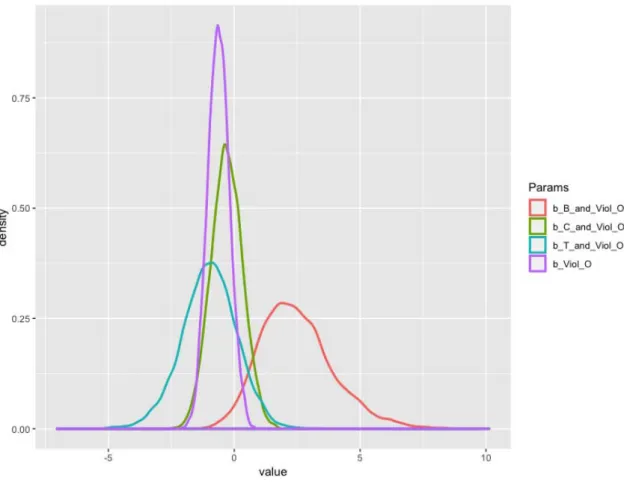
bvl_plotDensity(model, c("b_B_and_Viol_O", "b_C_and_Viol_O", "b_T_and_Viol_O", "b_Viol_O"))

(34)

34

Figure 9 - Density (Viol)

Overall, the results indicate that violence is not encouraged in the stories, as violence often bring bad outcomes for the main characters. The coefficient

b_Viol_O is negative, which suggests violence tends to go against the good

outcome for the main characters. This distribution is narrow, and with a good credibility range.

When considering violence together with the Three Teachings variable, we can see that the coefficients for Confucianism and Taoism are still negative. However, the coefficient for Buddhism and violence is positive, that means although the main character can commit a violent act, his or her outcome can still be favorable (positive coefficient).

Comparing violence and lying:

bvl_plotDensity2d(model, "b_Lie_O","b_Viol_O") We can have the pair parameter images as follow:

(35)

35 Hình 10

Both coefficients are negative, which indicates characters who have lied and committed violence tend not to have a good outcome.

If we compare the correlation between this pair of parameters, the coefficient for violence is much weaker than that of violence.

To compare the coefficients of Three Teachings elements with violence with each other:

bvl_plotDensity2d(model, "b_B_and_Viol_O", "b_C_and_Viol_O", color_scheme = "orange")

(36)

36 Figure 11

The results indicate different trends for Buddhism and Confucianism. It seems the outcome tends to be positive for characters that express the core values of

Buddhism yet commit violence. Nonetheless, the influence of Buddhism is much stronger.

bvl_plotDensity2d(model, "b_B_and_Viol_O", "b_T_and_Viol_O", color_scheme = "orange")

(37)

37 Figure 12

Similarly, there are different trends for Buddhism and Taoism. It seems Buddhism is more tolerant toward violent behaviors, while it is the opposite for Confucianism. Nonetheless, the influence of Buddhism is much stronger.

Next are the cofficients of Confucianism and Taoism:

bvl_plotDensity2d(model, "b_C_and_Viol_O", "b_T_and_Viol_O", color_scheme = "blue")

(38)

38 Figure 13

In Figure 13, Confucianism and Taoism’s coefficients are quite similar, and they are both small negatives, centered around the same range of value. One can infer Confucianism and Taoism don’t tolerate violence.

The results, as shown in Figure 11 and 12, indicate a propensity to tolerate violence from a character whose values are Buddhism. The propensity contradicts with Buddhism's values, which encourage humanity and compassion. In terms of Confucianism and Taoism, we can reluctantly interpret the results based on the values that Confucianism and Taoism characters hold. Confucianism characters are usually scholars, while Taoism characters value the ethics of "non-contrivance" or "effortless action". Thus, the characters will tend to avoid using violence to reach their goals.

Compare the correlations between the Three Teachings and lying behavior: First is the pair of Buddhism and Confucianism:

bvl_plotDensity2d(model, "b_B_and_Lie_O", "b_C_and_Lie_O", color_scheme = "orange")

(39)

39 Figure 14

Buddhism and Confucianism assume the same tendency in terms of correlation with lying behaviors and are distributed around the mean value. However, the coefficient of Buddhism is small, and the distribution lies between negative and positive. Thus, the results show Buddhism is not tolerant toward lying. On the contrary,

Confucianism elements have a strong positive coefficient, the entire 95% CI being positive.

Next, we consider Buddhism and Taoism in their relationship with lying behaviors:

bvl_plotDensity2d(model, "b_B_and_Lie_O", "b_T_and_Lie_O", color_scheme = "orange")

(40)

40 Figure 15

Similar to Confucianism, Taoism also predicts lying behaviors much stronger than Buddhism does.

The last pair to be compared is Confucianism and Taoism:

bvl_plotDensity2d(model, "b_C_and_Lie_O", "b_T_and_Lie_O", color_scheme = "blue")

(41)

41 Figure 16

In their relations to the lying behavior of the main characters, Taoism and Confucianism are quite similar and both center in the positive.

One important characteristic of Confucianism should be kept in mind when interpreting these results: Confucianism boasts teachings related to ambitions of becoming feudal officials, the latter often being an end that justifies all means – including behaviors such as lying.

Comparing situations with and without intervention:

The code for tests on variable Outcome (“O”) when there are and are not external elements intervening in the story yield two distribution graphs y_rep as follows.

bvl_plotTest(model, "O", "Int1_or_Int2_1") bvl_plotTest(model, "O", "Int1_or_Int2_2")

The following pair of graphs in Figure 17 corresponds to the values of Int1_or_Int2 in the above commands.

(42)

42 Figure 17a

Figure 17a plots the graphic representation of the relationship when

(43)

43 Figure 17b

The two graphs appear somewhat similar, meaning that the ending of a story does not depend significantly on the factor of external intervention. Besides, the

respective distributions of coefficients a_Int1_or_Int2[1] and

a_Int1_or_Int2[2] have the same curve pattern, suggesting that when there are

external interventions, improvements in main character behaviors compared to when there are no interventions are still negligible.

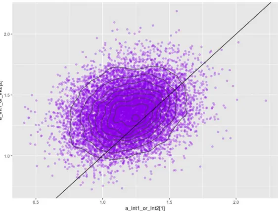
Figure 18

The relationship between changes of coefficients a_Int1_or_Int2[1] and

(44)

44 Figure 19

Figure 19 also shows that convergent values have rather even distributions, all positive, and are mostly distributed around a determined interval of values.

Update

The bayesvl R Package was officially published by CRAN on May 24, 2019, and can now be accessible from the CRAN web site:

https://cran.r-project.org/package=bayesvl [28].

Development Team

Members of the research team AISDL and SDAG have contributed to the

development of bayesvl at different stages of the project (data collection, program testing, result examination, manuscript writing). As of bayesvl v0.8.5, contributors to the development process include:

• Manh-Tung Ho

• Hong-Kong To Nguyen

• Manh-Toan Ho

• Hung-Hiep Pham

• Minh-Hoang Nguyen, and

(45)

45

Acknowledgments

AISDL and SDAG would like to acknowledge the financial support and data supply from Vuong & Associates, in particular from Director Dam Thu Ha and Nghiem Phu Kien Cuong.

The cover logo design of bayesvl is courtesy of artist Bui Quang Khiem.

References

[1] R Development Core Team. (2010). R: A Language and Environment for Statistical Computing. Vienna, Austria: R Foundation for Statistical Computing. Retrieved from http://www.R-project.org/

[2] Vuong, Q. H., & La, V. P. (2019). BayesVL package for Bayesian statistical analyses in R. Github: <https://github.com/sshpa/bayesvl>. Version 0.8.

[3] Ho, M. T., Vuong, Q. H. (2019). The values and challenges of ‘openness’ in addressing the reproducibility crisis and regaining public trust in social sciences and humanities. European Science Editing, 45(1), 14-17, DOI: 10.20316/ESE.2019.45.17021.

[4] Vuong, Q. H., Ho, M. T., & La, V.-P. (2019). ‘Stargazing’ and p-hacking behaviours in social sciences: some insights from a developing country. European Science Editing, 45(2), 54-55.

[5] Vuong, Q. H. (2018). “How did researchers get it so wrong?” The acute problem of plagiarism in Vietnamese social sciences and humanities. European Science Editing, 44(3), 56-58. doi:10.20316/ese.2018.44.18003

[6] Vuong, Q. H. (2017). Open data, open review and open dialogue in making social sciences plausible. Retrieved from http://blogs.nature.com/scientificdata/ 2017/12/12/authors-corner-open-data-open-review-and-open-dialogue-in-making-social-sciences-plausible/

[7] Vuong, Q. H., & Napier, N. K. (2017). Academic research: The difficulty of being simple and beautiful. European Science Editing, 43(2), 32-33; DOI: 10.20316/ESE.2017.43.002

[8] Vuong, Q.-H., Bui, Q.-K., La, V.-P., Vuong, T.-T., Nguyen, V.-H. T., Ho, M.-T., . . . Ho, M.-T. (2018). Cultural additivity: behavioural insights from the interaction of Confucianism, Buddhism, and Taoism in folktales. Palgrave Communications, 4(1), 143. DOI: 10.1057/s41599-018-0189-2

(46)

46

[9] Vuong, Q.-H., Bui, Q.-K., La, V.-P., Vuong, T.-T., Ho, M.-T., Nguyen, H.-K. T., . . . Ho, M.-T. (2019, 2019, January 26). Cultural evolution in Vietnam’s early 20th century: a Bayesian networks analysis of Franco-Chinese house designs. (Working Paper No. PKA-1901). arXiv Preprints, arXiv:1903.00817v1 [Stat.AP]. [10] Ho, M.-T., La, V.-P., Nguyen, M.-H., Vuong, T.-T., Nghiem, K.-C. P., Tran, T., . . . Vuong, Q.-H. (2019). Health care, medical insurance, and economic destitution: A dataset of 1,042 stories. Data, 4(2), 57, DOI: 10.3390/data4020057.

[11] Le, A.-V., Do, D.-L., Pham, D.-Q., Hoang, P.-H., Duong, T.-H., Nguyen, H.-N., ... Vuong, Q.-H. (2019). Exploration of youth’s digital competencies: a dataset in the educational context of Vietnam. Data, 4(2), 69, DOI: 10.3390/data4020069.

[12] McElreath, R. (2018). Statistical Rethinking: A Bayesian Course with Examples in R and Stan. London, UK: Chapman and Hall/CRC.

[13] Scutari, M. (2010). Learning Bayesian Networks with the bnlearn R Package. Journal of Statistical Software, 35(3), 1-22. doi:10.18637/jss.v035.i03

[14] Muth, C., Oravecz, Z., & Gabry, J. (2018). User-friendly Bayesian regression modeling: A tutorial with rstanarm and shinystan. Quantitative Methods for Psychology, 14(2), 99-119. DOI: 10.20982/tqmp.14.2.p099

[15] Gabry, J., & Goodrich, B. (2016). rstanarm: Bayesian applied regression modeling via Stan, R package version 2.10.0. Retrieved from

https://cran.rproject.org/web/packages/rstanarm/index.html

[16] Huu, N. V., Vuong, Q.-H., & Ngoc, T. M. (2005). Central limit theorem for functional of jump Markov processes. Vietnam Journal of Mathematics, 33(4), 443-461.

[17] Thao, H. T. P., & Vuong, Q.-H. (2015). A Merton model of credit risk with jumps. Journal of Statistics Applications and Probability Letters, 2(2), 97-103. DOI: 10.12785/jsapl/020201

[18] Vuong, Q. H. (2001). Black-Scholes PDE: A finance application. Paper presented at the International Conference on Differential Equation Approximation and Applications, November 2001, Vietnam National University and Institute of Mathematics.

[19] Vuong, Q. H., & Napier, N. K. (2014). Making creativity: the value of multiple filters in the innovation process. International Journal of Transitions and Innovation Systems, 3(4), 294-327. DOI: 10.1504/IJTIS.2014.068306

(47)

47

[20] Vuong, Q. H., Napier, N. K., & Tran, T. D. (2013). A categorical data analysis on relationships between culture, creativity, and business stage: the case of Vietnam. International Journal of Transitions and Innovation Systems, 3(1), 4-24.

[21] Vuong, Q. H., Ho, M. T., Nguyen, H. K., & Vuong, T. T. (2018). Healthcare consumers’ sensitivity to costs: a reflection on behavioural economics from an emerging market. Palgrave Communications, 4, 70, DOI: 10.1057/s41599-018-0127-3.

[23] Vuong, Q. H. (2015). Be rich or don’t be sick: estimating Vietnamese patients’ risk of falling into destitution. SpringerPlus, 4(1), 529, DOI: 10.1186/s40064-015-1279-x.

[24] Vuong, Q. H. (2019). The three teachings, lies, and violence in Vietnamese folktales: a dataset and simulations. Open Science Framework. Retrieved from: https://osf.io/kqhf9/

[25] Gelman, A., & Rubin, D. B. (1992). Inference from iterative simulation using multiple sequences. Statistical Science, 7(4), 457-472, DOI: 10.1214/ss/1177011136

[26] Brooks, S. P., & Gelman, A. (1998). General Methods for Monitoring Convergence of Iterative Simulations. Journal of Computational and Graphical Statistics, 7(4), 434-455, DOI: 10.1080/10618600.1998.10474787 [27] Lynch, S. M. (2007). Introduction to Applied Bayesian Statistics and Estimation

for Social Scientists. New York, NY: Springer.

[28] La, V.P, & Vuong, Q.H. (2019). bayesvl: Visually Learning the Graphical Structure of Bayesian Networks and Performing MCMC with 'Stan'. The Comprehensive R Archive Network (CRAN): <https://cran.r-project.org/package=bayesvl>; version 0.8.5 (May 24, 2019).