A new deep reinforcement learning architecture for autonomous UAVs

BACHELOR DEGREE THESIS

TFG TITLE: A new Deep Reinforcement Learning architecture for autonomous UAVs DEGREE: Grau en Enginyeria Telem`atica

AUTHORS: Guillem Mu ˜noz Ferran ADVISOR: Cristina Barrado Mux´ı DATE: 31 d’agost de 2018

Title : A new Deep Reinforcement Learning architecture for autonomous UAVs Authors:Guillem Mu˜noz Ferran

Advisor: Cristina Barrado Mux´ı Date: August 31, 2018

Overview

Recent improvements in computation and algorithmic research, together with the rising era of Big Data, have allowed Artificial Intelligence increase its popularity within masses. The recent publication of the Deep Q-Network (DQN) algorithm, which combines Q-learning with deep neural networks, has been demonstrated as being able to learn how to solve complex task, such as playing Atari games, in an unknown environment solely by gath-ering experience. These conditions open the door for many other applications, such as autonomous vehicles, doctors or production chains. Moreover, the preceding work of this project was focused on building a baseline architecture for enabling Unmanned Aerial Ve-hicles (UAVs) learn how to behave autonomously.

In this project we provide different architectures for scaling this solution. To evaluate the convergence of the algorithm, we create challenging tasks concerning obstacle avoidance and goal position reaching inside a realistic simulated environment. The provided solu-tion allows UAVs to autonomously move in three dimensions as well as controlling and modifying their velocities. Modifications in the architecture provide different approaches for learning, which are evaluated together with its training efficiency metrics and testing results.

The development has been focused on integrating Deep Learning and Reinforcement Learning tools such as Keras and OpenAI Gym in order to build a modular and acces-sible framework capable of training and testing DRL models for autonomous UAVs within simulated environments. Results of the carried experiments show multiple enhancements compared to previous research and work, along with providing useful insights for poten-tially identified improvements. In this project, we have been able to successfully beat the existent baseline Double Deep Q-Learning architecture for autonomous UAVs, obtaining a 49% more of average reward and no collisions, on a non-trivial task within a realistic simulated environment.

T´ıtulo: A new Deep Reinforcement Learning architecture for autonomous UAVs Autores: Guillem Mu˜noz Ferran

Director: Cristina Barrado Mux´ı Fecha: 31 d’agost de 2018

Resumen

Millores recents en les `arees d’investigaci´o de la computaci´o i l’algor´ıtmica, juntament amb la creixent era del Big Data, han perm`es a l’Intel_·lig`encia Artificial guanyar popularitat entre les masses. La recent publicaci´o de l’algorisme Deep Network (DQN), que combina Q-learning amb xarxes neuronals profundes, ha demostrat ser capac¸ d’aprendre a resoldre tasques complexes, com jugar a jocs d’Atari, en un entorn desconegut i nom´es a trav´es de l’experi`encia. Aquestes condicions obren la porta per a moltes altres aplicacions com vehicles, doctors o cadenes de producci´o aut`onomes. La tesi pr`evia a aquest projecte va estar focalitzada en construir una arquitectura base, habilitant vehicles aeris no tripulats (UAVs) a aprendre com comportar-se de manera aut`onoma.

En aquest projecte prove¨ım aquella soluci´o de diferents arquitectures per tal d’escalar-la. Per a evaluar la converg`encia de l’algorisme, creem tasques desafiants consistent en evi-tar obstacles i en arribar a una destinaci´o, dins d’un entorn de simulaci´o realista. Aquesta soluci´o permet a UAVs moure’s de manera aut`onoma en tres dimensions, a m´es de po-der variar i controlar la seva velocitat. Les modificacions de l’arquitectura proporcionen diferents enfocaments per a aprendre. Tots s´on avaluats amb l’efici`encia de les m`etriques d’entrenament i els resultats satisfactoris de les proves.

El desenvolupament ha estat centrat en integrar eines de Deep Learning i Reinforcement Learning com Keras o OpenAI Gym amb la finalitat de construir un framework modular i accessible capac¸ d’entrenar i provar models de DRL per a UAVs aut`onoms en entorns simulats. Els resultats dels experiments portats a terme mostren m´ultiples millores en comparaci´o amb el treball i la investigaci´o pr`evia, proporcionant a m´es idees ´utils per a millores potencials identificades. En aquest projecte hem aconseguit superar amb `exit l’arquitectura de Double Deep Q-Learning anterior per a UAVs aut`onoms, obtenint un 49% m´es de recompensa mitjana i sense cap col·lisi´o, en una tasca no trivial i dins d’un entorn de simulaci´o realista.

Acknowledgements

Years ago back in my childhood, I remember falling in love with maths. My passion for engi-neering and computer science made me start this degree in networks and telecommunications. Almost a year ago, motivation brought me to study machine learning. But the key factor in this thesis has been inspiration. Cristina Barrado, my supervisor, has inspired me in working hard for what you love and what you aim, leaving aside other external factors.

I would like to thank also people who supported me during this whole journey, including my family, friends and girlfriend. Deep inside myself I know one day I will end up pursuing a doctorate, but until now, this thesis describes somehow my small piece of contribution to science and research.

Declaration

This thesis has been totally developed, conducted and written by myself. All external sources both used or applied have been carefully declared in the text with a formal reference. This thesis is only used for theGrau en Enginyeria Telemàticacarried atEscola d’Enginyeria de Telecomunicacions i Aeroespacial de Castelldefels(EETAC) belonged to theUniversitat Politècnica de Catalunya(UPC).

Guillem Muñoz August 2018

Contents

List of Figures xi

List of Tables xiii

Nomenclature xvi

1 Introduction 1

1.1 Artificial intelligence . . . 1

1.2 Autonomous UAVs . . . 2

1.3 Baseline of this work . . . 3

1.4 Project objectives . . . 4

1.5 Project outline . . . 4

2 Reinforcement learning 6 2.1 Introduction . . . 6

2.2 Agent-environment scheme . . . 7

2.3 Markov Decision Process . . . 8

2.4 Value functions . . . 9

2.5 Classifications . . . 11

2.6 Temporal difference learning . . . 12

2.7 Q-learning . . . 13

3 Deep reinforcement learning 16 3.1 Neural networks in RL . . . 16

3.2 Deep Q-Network . . . 18

3.3 Double DQN . . . 22

4 Materials and methods 24 4.1 Tools . . . 25

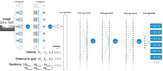
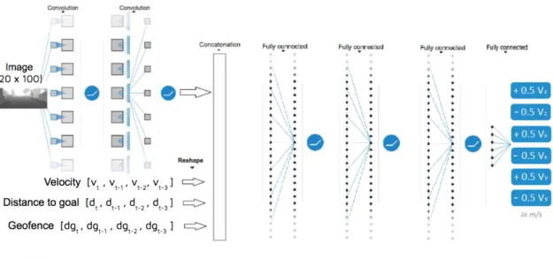
viii Contents 4.1.1 AirSim . . . 25 4.1.2 OpenAI Gym . . . 26 4.1.3 Keras-rl . . . 27 4.2 Checkpoints . . . 27 4.3 Agent-environment design . . . 28 4.3.1 The environment . . . 28 4.3.2 Actions . . . 31 4.3.3 Rewards . . . 33 4.3.4 States . . . 33 4.4 Joint Q-network . . . 36 4.4.1 Initial approach . . . 36 4.4.2 Velocity JNN . . . 39 4.4.3 Time sensitive JNN . . . 40 4.5 Front-End prototype . . . 40 5 Results 43 5.1 Set-up . . . 43 5.2 JNN vs CNN . . . 44 5.2.1 Training metrics . . . 45 5.2.2 Testing results . . . 45 5.3 Performance of JNN variations . . . 48 5.3.1 Training metrics . . . 48 5.3.2 Testing results . . . 50 5.4 Looking forward . . . 52

5.4.1 Prioritized experience replay . . . 52

5.4.2 Transfer learning . . . 53

6 Conclusions 54 Bibliography 56 Appendix A Deep learning 61 A.1 Introduction . . . 61

A.2 Convolutional neural networks . . . 62

A.2.1 Fully-connected . . . 62

A.2.2 Activation . . . 63

Contents ix

A.2.4 Spatial Pooling . . . 65

A.2.5 Neural network set-up . . . 66

A.2.6 Convolutional architectures history . . . 66

Appendix B Previous scenario 68 B.1 Baseline architecture . . . 68

B.1.1 The environment . . . 68

B.1.2 Actions . . . 69

B.1.3 Rewards . . . 69

B.1.4 States . . . 70

List of Figures

2.1 Reinforcement learning basic scheme, the agent-environment interaction. . 7

3.1 Example of a binary image classification problem using a convolutional neural network in order to decide whether a drone is flying over a private propierty or the public space. . . 17

3.2 Example of an agent that following an optimal policy maps each state (repre-sented by an image) into two possible actions, moving forward or rotating. . 17

3.3 CNN architecture for DeepMind DQN playing Atari games [MKS+_{15]. The} input to the neural network consists of an 84 X 84 X 4, followed by three convolutional layers and two fully connected layers with a single output for each valid action. Each hidden layer is followed by a rectifier nonlinearity (ReLU) . . . 20

3.4 Pie chart exposing a comparative analysis on game performance for DQN and human testers. . . 21

3.5 Colors are chosen relative to green seen as a better performance for DQN and red seen as a worse performance for DQN. . . 22

4.1 Overview of agent-environment interaction using our DRLD BackEnd . . . 25

4.2 AirSim Neighborhood environment views. . . 28

4.3 Geo-fencing limits for our quadcopter. . . 30

4.4 UAV possible movements within the environment. . . 32

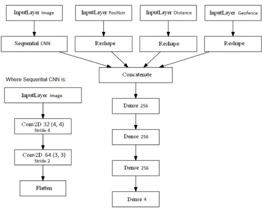
4.5 Layers of the two models shown in cascade view. . . 37

4.6 Architecture of the multiple input neural network . . . 37

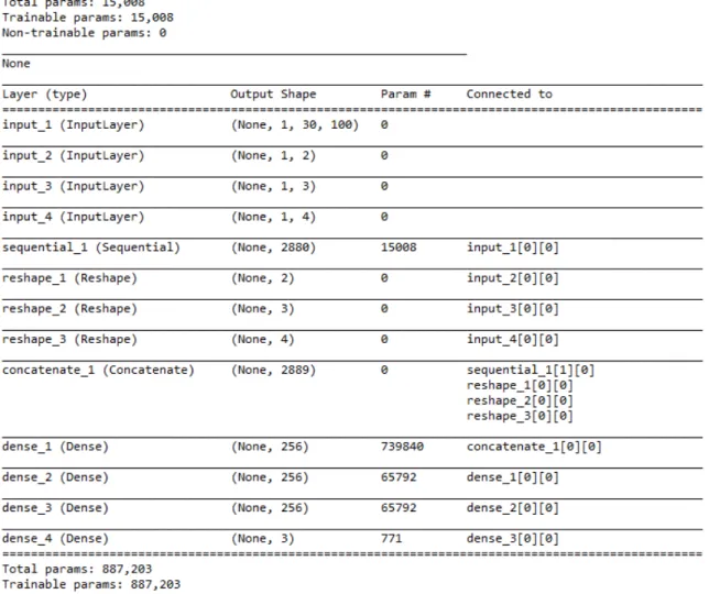
4.7 Details on the neural network architecture. TheNoneparameter in the Output Shape is used for accepting tensors with dynamic dimensions due to when usingKerasyou can useTensor f loworT heanoas backend libraries. . . . 38

4.8 Modified JNN architecture for three dimensional UAVs and velocity oscillation. 39 4.9 JNN architecture with time progressive values. . . 40

xii List of Figures

4.10 Front-end prototype built for training and testing user interface. . . 41

4.11 Prototype solution in a research production environment. Note that the brain icon emulates the whole deep reinforcement learning core within the Back-End, within the interaction of Gym and Keras-rl libraries. . . 42

5.1 Values regarding cumulative reward obtained during training phase. Vertical discontinuous line represents until which number of stepseis annealed to its final value. . . 45

5.2 Testing episodes using the CNN model. Green dots refer to goal achieved episodes and the opposite for red ones. . . 46

5.3 Testing episodes using the JNN model. Green dots refer to goal achieved episodes and the opposite for red ones. . . 47

5.4 Test comparison between models. . . 47

5.5 Training graphs comparison between the V1 and the T1 architectures. . . . 49

5.6 Training graphs comparison between V4 and T4 scenarios. . . 49

5.7 Additional training graphs for the V1 architecture. . . 50

A.1 Scheme of a biological neuron and its mathematical model . . . 63

A.2 A comparison of the most common non-linear activation functions . . . 64

B.1 Unreal environment modified from Blocks. Measures are in meters . . . 68

B.2 State representation composed of depth image and encoded track angle. Measures are in pixels. . . 71

B.3 Architecture of the convolutional neural network. Note that the third con-volutional layer was found not to contribute to abstraction or decrease in parameter size with a kernel of 1 x 1 and stride of 1 too, but was kept to preserve the original amount of layers of [MKS+_{15]. . . . 71}

List of Tables

4.1 Data fetched from the simulation environment at every time-step. . . 29 5.1 Hyperparameters of the agent implementation for both models . . . 44 5.2 Different training values from modifications of the general JNN architecture. 48 5.3 Testing results for the two one-destination different architectures. . . 50 5.4 Testing results for the two four-destination different architectures. . . 51 B.1 Data fetched from the simulation environment at every time-step . . . 69

Nomenclature

A(s) set of all possible actions in states– action space S set of all states – state space

a action

r reward

s,s0 state

At action at time stept

Gt return (cumulative discounted reward) following time stept

Rt reward at time stepttoSt 1andAt 1

St state at time stept

T final time step of an episode – terminal step

t discrete time step

µ behaviour policy used to select actions while estimating values for policyp p policy, decision-maker

p_⇤ optimal policy

dt temporal-difference error att

q,qt vector of weights underlying an approximate value function

q vector of weights of the target network ˆQ

Q,Qt array estimates of action-value functionqp orq⇤

q_⇤(s,a) value of taking actionain statesunder the optimal policyp_⇤ q_p(s,a) value of taking actionain statesunder policyp

V,Vt array estimates of state-value functionvp orv⇤ v_⇤(s) value of statesunder the optimal policyp_⇤ v_p(s) value of statesunder policyp (expected return) yt learning target

Nomenclature xv q(s,a;q) approximate value of state-action pairs,agiven weight vectorq

v(s;q) approximate value of statesgiven weight vectorq

a learning rate or step-size parameter

e probability of taking a random action in ane-greedy policy

g discount factor

t target factor

argmax_af(a) a value ofaat which f(a)takes its maximal value .

= an equality relationship that is true by definition

E[X] expectation of random variableX

Pr_{X=x_} probability that the random variableX takes on the valuex

f agent’s relative heading to the goal – track

y yaw angle relative to initial orientation

dx agentsxdistance with goal

dy agentsydistance with goal

dz agentszdistance with goal

dgx agents distance withxgeofencing

dgy agents distance withygeofencing

dgz agents distance withzgeofencing

px agents globalxposition

py agents globalyposition

pz agents globalzposition

vx agentsxvelocity

vy agentsyvelocity

vz agentszvelocity

AGI Artificial General Intelligence

AI Artificial Intelligence

API Application Programming Interface

CNN Convolutional Neural Network

DDQN Double Deep Q-Network

DQN Deep Q-Network

DRL Deep Reinforcement Learning

xvi Nomenclature

JQN Joint Q-Network

MC Monte Carlo

MDP Markov Decision Process

RL Reinforcement Learning

RPC Remote Procedure Call

TD Temporal Difference

UAS Unmanned Aerial System

Chapter 1

Introduction

1.1 Artificial intelligence

Artificial intelligence (AI) is a field of computer science that aims to enabling computer systems encapsulate cognitive functions. This involves including adaptive and learning capabilities which lead the systems to a self-improved state. In computer science, AI research is defined as the study ofintelligent agentsany system that perceives its environment and takes actions that maximize its chance of successfully achieving its goals.

When looking into new paradigms, in [Vin93] Vernor Vinge explains the concept of Singularity, the possible causes and how humans may survive after it. The Singularity involves a self evolving intelligence which can improve more rapidly than one could ever imagine. This artificial super intelligence possesses more cognitive capabilities than gifted to humans beings. Back to 1993, Vinge already stated:

“Within thirty years, we will have the technological means to create superhuman intelli-gence. Shortly after, the human era will be ended.”

A similar approach of what Nick Bostrom shows in [Bos14], where he suggests that new super intelligence could replace humans as the dominant lifeform, besides defining super intelligence as:

“an intellect that is much smarter than the best human brains in practically every field, including scientific creativity, general wisdom and social skills.”

Experts in the field remark that the first super intelligent machine will be the last invention that human may ever need to make, but that there is a long road ahead in order to potentially reach this point. Recent research advances include the distinction between two main types of artificial intelligence.

Artificial General Intelligence (AGI)predicted to happen around 2040 by [RKT18], when an intelligence which can be as intelligent as human beings would be ready. Experts

2 Introduction explain that there is not a predefined definition of it and that it should be able to learn, represent knowledge, plan, take decisions under uncertainty, communicate in a natural language and use these skills towards common goals to be an AI-complete machine. The biggest constraint here is being able to figure out how the human brain, a 20 W machine product of millions of years of evolution, actually works. So, even if we are able to find out how a single neuron or a set of them work, we are far away of understanding the brain in its fullness.

Instead, Weak Artificial Intelligence stands for an AI designed to solve a specific problem. Even AlphaGo [SHM+_{16] [SSS}+_{17], a computer program developed by DeepMind}

and one of the most important accomplishments in AI research due to its complexity and innovation, is considered to be a narrow AI (Weak AI).

Moving away from Weak Artificial Intelligence to AGI is a complex journey but neural networks are easing it up. DeepMind has also recently submitted a paper calledPathNet: Evolution Channels Gradient Descent in Super Neural Networks[FBB+_{17] which could be}

the stepping stone of first artificial general intelligence.

Artificial intelligence is not a recent concept. The first work that is now generally recognized as AI was [MP43] formal design for Turing-complete artificial neurons, dated in 1943, and the field of AI research was born at a workshop at Dartmouth College [JMS18] in 1956.

So, what conditions are different that have lead to a recent growth in AI research? Essentially three factors, almost unlimited computing power, more efficient algorithms and enormous amount of data available. The work in this project will be mainly focused on the second concept and the development will be around last innovative AI publications.

1.2 Autonomous UAVs

Research in the field of Unmanned Aerial Vehicles (UAV) is known to be one of the most interesting races in both academic and industrial environments. Considering its multiple applications including package delivery, aerial photography, industrial inspection, surveil-lance, zone control or monitoring and much more, there is a broad space for innovation and progress [VV14].

UAVs distinguish themselves from classic aircraft in being controlled by a remote operator instead of a on-board pilot. UAVs are usually guided by GPS signals which involve map errors and uncertainty. Instead of the requirements of human remote interaction, artificial intelligence is recently rubbing the point of achieving completely autonomous vehicles by the time this project is being written. The fundamental aspect of autonomous vehicle guidance is

1.3 Baseline of this work 3

trajectory planning. Historically, two fields have contributed to trajectory or motion planning methods: robotics, and dynamics and control [GKM10].

The main difference between automatic and autonomous control is that, in the first one, the engineer designing the goal needs to perfectly define everything beforehand in order for the UAV to solve it. Instead, in autonomous control, the UAV learns how to achieve the goal itself, with artificial intelligence, without predefining how to achieve the task, and the human interaction is only required in order to give the UAV the sufficient information to learn. Reinforcement learning (RL)methods, the core of this project, enable a vehicle to autonomously discover an optimal behaviour through trial-and-error interactions within the environment it is surrounded by.

Nevertheless, memory and computational complexity constraints affect reinforcement learning scalability. Throughout this project, the use ofdeep learningwill arise in order to address and overcome this issues, enabling reinforcement learning methods to scale to problems that were previously intractable. The use of deep learning algorithms together with RL defines the field ofdeep reinforcement learning (DRL), the enabler of this work.

1.3 Baseline of this work

In order to set up the objectives and goals of this project, it must be clearly distinguished what were the previous accomplishments regarding past research. Over his master project [Ker18], Kjell Kersandt built up the first prototype of a DRL framework for autonomous UAVs.

Supervised also by Cristina Barrado, the project ended up in a huge success. Besides building and setting up the framework for UAV simulations, final results came near human performance, in a similar comparison to what DeepMind published in [MKS+_{15], being it}

the major source for the development of the project. During this work, simulations were performed in a narrow custom environment, with a fixed altitude for the UAV and only one simple task to perform. While the overall performance remained below the human-level of comparison, potential improvements on several aspects that could lead to even higher reliability and finally a superhuman performance, were clearly identified.

The project covered the state-of-the-art DRL theory and perfectly reported a detailed research comparison on available implemented algorithms, enabling further research to be easier and more comprehensible.

4 Introduction

1.4 Project objectives

The main objective of this project, is and has been during its entire development, to learn. Learning how we, as humans, can build intelligent systems able to automate a task and perform it at a better level than our capacities.

At a more practical level, this project clearly involves different objectives. The two major ones are scaling the baseline work to a near-real simulated environment, and enhancing the current architecture in order to solve an autonomous task at a near-human performance.

Research is focused on the joint of computer vision and deep reinforcement learning, understanding and evaluating how to improve the way neural networks perceive and gather more information in DRL methods, rather than the mathematical algorithm itself. Among all this, the project involves also a lot of dedication in software development plus long training and testing simulations, enabling the UAV to behave in a more realistic way.

Other more technical objectives include a research in timing versus efficiency in deep learning models, checkpoints of best training models, geofencing intelligence, real control inside UAVs dynamics and much more which will be better explained in the course of the project itself.

1.5 Project outline

In order to better describe what will be presented in each chapter of this project, an outline is provided emphasizing the important aspects of each one:

Chapter 2 (Reinforcement learning)

introduces mathematical and theoretical concepts of reinforcement learning. It focuses on the previous knowledge one must acquire in order to comprehend future advances above historical algorithms. It does not intend to cover all methods of reinforcement learning but to overview the ones required for the project purpose.

Chapter 3 (Deep reinforcement learning)

the chapter comes up with the matter of the project, deep reinforcement learning. It explains the DQN algorithm published by DeepMind, a Google company, displaying also a personal analysis on the results obtained. Additionally, it presents the Double DQN, an improvement on the base algorithm.

Chapter 4 (Materials and methods)

summarizes how the development of the project has been made, what tools have been used and what research has been focused on. In an organized and brief manner, it shows

1.5 Project outline 5

how all the methods and tools integrate together in an unique framework. Reshuffles from scratch the way to approach the initial task and provides a totally new architecture based on the improvements and extensions proposed beforehand.

Chapter 5 (Results)

displays the final results with an extended comparison. Ultimately, evaluates the direction and track for future research in the field.

Chapter 6 (Conclusions)

closes the project with an evaluation of the final and most important aspects together with analyzing the accomplishment of the initial objectives.

Chapter 2

Reinforcement learning

This chapter is structured in the basic concepts for understanding reinforcement learning problems, but at some point it directly sticks to the most important pieces for this thesis. Noticeably, reinforcement learning is a complex and broad area in which we do not have enough opportunity to overview all methods and approaches. The best way for immersing into reinforcement learning is taking a look at [SB98] and the previous "state-of-the-art" work of this thesis carried in [Ker18].

2.1 Introduction

Supervised learning is nowadays the most used type of machine learning, a particular subfield of artificial intelligence. In supervised learning, the learner is typically provided with two sets of data, a training set and a test set, yet sometimes part of the training data is used as a validation set. To actually learn, the idea is to provide the learner with a set of well labeled examples in the training set. As labeled is meant the fact that they have been previously well classified by humans. The goal for the learner is to develop a rule to classify unlabeled examples in the test set with the highest possible accuracy and the lowest possible loss.

From speech automated systems, mail spam detection, weather prediction or hand-writing recognition to image classification are just some of the clear examples of supervised learning. However, for many problems of interest, the paradigm of supervised learning does not provide enough flexibility to solve the problem.

Whilst supervised learning problems receive an instructive feedback, in other words, it tells you how to achieve your goal, in reinforcement learning problems, an evaluative feedback is received, telling the agent how well it has achieved the goal.

In the image classification example, an instructive feedback is received. When the algorithm developed attempts to classify a certain image sample, it is directly told what true

2.2 Agent-environment scheme 7

class is. If an evaluative feedback had been returned, the classifier would have received a certain score in classifying the image, e.g.+20 points. But, without any more context, what

does receiving+20 points means?

This evaluative process leads to the ability of implementing a more complex, intuitive and accessible system. Maybe those+20 meant that a good decision was made, or further

iterating with the environment we find that it was a poor score.

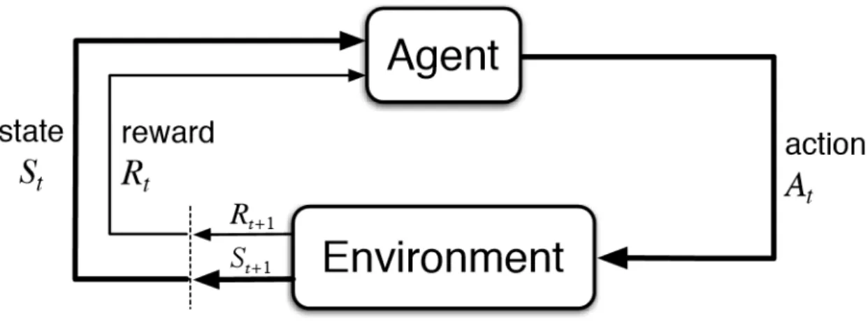
2.2 Agent-environment scheme

Reinforcement learning problems are based in learning how to achieve a certain goal from interaction. The most important components are theagent, which is basically the learner and decision-maker, and the conditions or surroundings with whom theagentinteracts, formerly called, theenvironment. This interaction is carried during a sequence of discrete time stepst. At each time step, theagentis in statest from the state spaceSand chooses which action

at to take from the set of possible actions in the action spaceA(st). Theenvironmentthen

responds with a new statest+1and a numerical rewardrt+1.

As it will be seen later, theagentcan choose which action to take in a given state, which has a significant effect on the next state it will see. However, the agent does not control the dynamics of the environment completely.

By taking a look at Figure 2.1, the general idea can be understood. The states are the basis for theagentto make the choices, the actions are the choices itself and the rewards are the basis for evaluating these choices.

8 Reinforcement learning In the end, the ultimate goal of theagent is to, at each time stept, map from states to probabilities for selecting each possible action. This mapping is called thepolicy and is denotedpt, where(pt(a|s)is the probability thatat=aifst =s.

pt(a|s) =P(at =a|st =s) (2.1)

2.3 Markov Decision Process

RL states satisfy the Markov property:

A statesis said to satisfy theMarkov propertyif the future is independent of the past given the present. In other words, the current states describes all the past states and is sufficient for successive states. In probability theory and related fields, aMarkov process, is a stochastic process that satisfies theMarkov property[Ser09] [ER12].

AMarkov process(orMarkov chain) is a tuplehS,P_i

• Sis a (finite) set of states

• Pis a state transition probability matrix,

P(s0|s) =Pr[St+1=s0|St=s] (2.2)

More in depth, aMarkov reward processis aMarkov processwith value judgments. This basically shows how much reward is accumulated across some particular sequence that is sampled from aMarkov process.

AMarkov reward processis a tuplehS,P,R,g_i

• Ris a reward function,

Rs=E[Rt+1|St =s] (2.3)

• g is a discount factor,

g 2[0,1] (2.4)

Equation 2.3 shows that when being in a states, how much reward do we get for being in that state only. It is just the immediate reward. But actually, what we look forward to in

2.4 Value functions 9

reinforcement learning is the cumulative sum of these rewards, noted asGt in equation 2.5,

referencing thegoal.

Gt=. Rt+1+gRt+2+g2Rt+3+...= •

Â

The discount factorg sets up the balance between immediate and future rewards. A factor near 0 will make the agent "myopic" by only considering immediate rewards, while a factor approaching 1 will make it strive for a long-term high reward, more "far-sighted".

With all this information, we are able to randomly sample those transitions and compute, but in this scheme there is not any agent making decisions. In order to solve the reinforcement learning problem, we need to look for one more piece of complexity, actions. And all this sets up what is called aMarkov decision process(MDP).

AMarkov decision processis a tuplehS,A,P,R,gi

• Ais a finite set of actions,

• Pis a state transition probability matrix,

P(s0|s,a) =Pr[St+1=s0|St =s,At=a] (2.6)

• Ris a new reward function,

Ra_s =E[Rt+1|St=s,At =a] (2.7)

Clearly, both the transition probability matrix and the rewards now depend on which action is taken. So, where you end up, depends on the chosen actions throughout the process. Formally, there will be one separatePfor each action.

2.4 Value functions

The value function is used for the agent to estimatehow goodis to be in a particular state. It is defined with respect to a policy, since the rewards the agent can expect to receive in the future depend on the action it takes. The value of a statesunder a policyp is the expected reward

10 Reinforcement learning when starting insand followingpand it is denoted asv_p(s), calledstate-value function for policyp and defined as

v_p(s) =E_p[Gt|St=s] =Ep " _•

Â

whereEp[·] denotes the expected value of a random variable. In a similar way, qp is

defined as theaction-value function for policypfor taking actionain statesunder policyp:

q_p(s,a) =E_p[Gt|St =s,At =a] =Ep " _•

Â

TheBellman equationis the formal expression of the recursive relationship between the value of a state and the value of its successor states that value functions satisfy induced by the Markov property. TheBellman equationforvp is formally expressed in 2.10 equation,

vp(s) =

Â

a p(a|s)

Â

p(s0,r|s,a)[r+gvp(s0)],8s2S. (2.10)

The equation states that the value of the starting state must be equal to the discounted value of its expected next state plus the reward, averaging over all the possibilities and weighting each of them by is occurrence probabilities.

Noticeably, the objective of RL is to find the policy that maximizes the reward over the long run. In evaluating policies, policyp is considered to be better or equal to a policyp0

if the expected return of that policy is greater than or equal to that ofp0_{for all states. For}

finite MDPs, there is at least one policy that fulfills this previous statement against all other policies, calledoptimal policyand denotedp_⇤.

In consequence, theoptimal state-value functionis denotedv_⇤and is defined as:

v_⇤(s)=. max

p vp(s),8s2S (2.11)

The same goes for theoptimal action-value function, denotedq_⇤and defined as:

q_⇤(s,a)=. max

p qp(s,a),8s2S,a2A (2.12)

Taking this into account, equation 2.10 can be written into the Bellman optimality equationfor bothv_⇤andq_⇤[SB98].

2.5 Classifications 11

2.5 Classifications

Environment knowledge

Finite MDPs are distinguished betweenmodel-based andmodel-freeproblems. A model-basedapproach has full knowledge of all possible statesS, actions A(st), state-transition

probabilitiesP(s0|s,a)and immediate rewardsrt+1. Noticeably, amodel-basedproblem can

be solved by algorithmic planning prior to simulation.

Clearly, this is highly limited and only leads to fully-knowledgeable processes. However, actual reinforcement learning methods are able to solve problems without previous knowledge about the environment. Those are calledmodel-freeproblems, where the agent has to gather experience by interacting with the environment. This approach is excellent for enabling UAVs to perform autonomous tasks and adapt to new environments.

Exploration vs exploitation

Since reinforcement learning was developed so as to emulate human learning styles, this explanation gets easier by figuring an example. In life, we learn a lot through the years. Since we are young, education teaches us to search for our career options, to both find what we like and see what we are good at.

Two ways to face this search can be adopted. You canexploremore and always look for different options, or you can settle on an option,exploitingwhat you already know. The same goes for RL. When the agent explores more, it takes risks in the process and exposes to more failures. But when it stops exploring, it settles on something, and it is possible that this is not the best option and there is something better out there. The agent risks not searching for other option that could be potentially more beneficial in the long run.

This trade-off has existed during decades and will still exist, maybe because there is not a certain solution and it always depends on the situation. Later in this chapter, an approach to solve this dilemma for our system is introduced.

On-policy vs off-policy

In order to further address the problem introduced above, two different approaches are grouped,on-policyandoff-policylearning methods.

Inon-policylearning, the agent commits to always have an exploring part, and therefore tries to find the best policy that still explores. On the other way,off-policymethods use two different policies, one that is learned about and becomes the optimal policy, calledtarget

12 Reinforcement learning

policyp, and one that is more exploratory and is used to choose the actions and generate behaviour, calledbehaviour policyµ.

Both learning approaches hold their advantages and drawbacks, and it also depends on the explicit algorithm used. This project will be focused mainly in a type ofoff-policylearning method due to the recent research progress over these areas.

2.6 Temporal difference learning

Temporal difference(TD) methods aremodel-freelike Monte-Carlomethods and update estimates on the basis of learned estimates, analogous to dynamic programming. Both concepts are extensively explained in [SB98]. UnlikeMonte-Carlomethods, TD methods do not have to wait until the end of an episode to determine the increment toV(St)with the

actual returnGt.

Instead, TD methods just wait until the next time step and use anestimatedreturn equal to

Rt+1+gV(St+1). With the immediate rewardRt+1and the estimate forV(St+1), TD methods

directly form a target and make an useful update. The value functionV(St)update toward

the estimated returnRt+1+gV(St+1)is defined as:

V(St) V(St) +a[Rt+1+gV(St+1) V(St)] (2.13)

wherea is thelearning rate. The difference between the estimated value ofV(St)and

the following better estimate Rt+1+gV(St+1), which is based on the agent’s immediate

experience, is calledTD errorand denoteddt:

dt=Rt+1+gV(St+1) V(St) (2.14)

So, as Monte-Carlo methods, TD methods follow the pattern of generalized policy iteration [VDW78] but inMonte-Carlothe error obtained is equivalent to the sum of all TD errors for every time step until the end of the episode. Depending on the application and number of steps per episode, delaying all learning until the end of a long episode introduces a high variance, therefore can be critical for some systems.

TD methods open up a new paradigm because they can be implemented in an online, fully incremental way and several resources have shown a much faster convergence than MC ones [Sut88].

2.7 Q-learning 13

2.7 Q-learning

In order to explain theQ-learningalgorithm, which is the theoretical base of this thesis, a few premises are required to be introduced beforehand.

Action-value function

When facing model-based problems, state values are sufficient to find an optimal policy. However, inmodel-freeproblems, having the optimal action-value (values of state-action pairs) function q_⇤ avoids the agent to do a one-step-ahead search. This is because q_⇤

effectively catches the results of all one-step-ahead searches: for any given statesit is able to find an action that maximizesq_⇤(s,a). In other words, if you are usingmodel-freelearning,

it is better to estimate action valuesQ(s,a)instead of the state valuesV(s).

The action-value function allows optimal actions to be selected without knowing anything about possible successor state values and ables TD learning to converge faster to an optimal policy [SB98].

e-Greedy: Behaviour policy

In order to maintain the exploration versus exploitation trade-off, the use ofe-greedy policy

[TP11] as a behaviour policy was reported to be hard to beat [VM] and often the method of first choice [SB98] instead of more complex methods.

It relies on a simple but effective method, in which the amount of exploration is globally controlled by a parametere. Its main advantage is the suitability for large or even continuous state-spaces, due to no memorization of exploration specific data is required. Equation 2.15 formalizes thee-greedy policy,µ(St).

µ(St) = 8 < : argmax_aQ(St,A) at probability 1 e randomA at probabilitye (2.15) The algorithm

Q-learning algorithm introduces a fully implementable TD method within an off-policy approach. At each statest the actual actionAt is chosen with respect to the behaviour policy

14 Reinforcement learning have been selected with respect to the target policyp. The action value for starting statest

with actionAtis updated towards this alternative actionA0:

Q(St,At) Q(St,At) +a[Rt+1+gQ(St+1,A0) Q(St,At)] (2.16)

Since the target policypimproves greedy with respect toQ(s,a)and the behaviour policy µ improves with exploratory e-greedy with respect toQ(s,a), the TD control Q-learning

algorithm [WD92] is formulated as:

Q(St,At) Q(St,At) +a[Rt+1+gmax_a Q(St+1,a) Q(St,At)] (2.17)

As deduced from (2.13), the quantity in brackets expresses the TD error dt of the

Q-function:

dt =Rt+1+gmax_a Q(St+1,a) Q(St,At) (2.18)

The main idea is that the Q-learning method evaluates if the action taken by the behaviour policy is better or worse than the target policy, which approximates the optimal action-value functionq_⇤. Qhas been shown to converge toq_⇤with probability 1 [Sut88].

The original Q-learning pseudo-code (in Algorithm 1) summarizes all the concepts discussed above:

Algorithm 1Q-learning: An off-policy TD control algorithm

1: InitializeQ(s,a)randomly 2: Initialize discount factorg 3: Initialize step-size parametera 4: repeat(for each episode): 5: Observe initial stateS1

6: repeat(for each step of episode):

7: Choose actionAt using policy derived fromQ(e.g.e-greedy)

8: Take actionAt

9: Observe rewardRt+1and new stateSt+1

10: Q(St,At) Q(St,At) +a[Rt+1+gmaxaQ(St+1,a) Q(St,At)]

11: St St+1

12: untilSt is terminal

2.7 Q-learning 15

Q-learning has been classified as an adaptive control algorithm that is able to converge online to the optimal solution for completely unknown systems [LVV12].

Chapter 3

Deep reinforcement learning

3.1 Neural networks in RL

Using deep learning with reinforcement learning is what sets up deep reinforcement learning. The use of neural networks in reinforcement learning as function approximators for high-dimensional inputs was introduced by Paul J. Werbos, the scientist who first described the process of training neural networks trough backpropagation errors. In [Wer89] Werbos trains a neural network by error backpropagation to learn policies and value functions using temporal difference algorithms.

Although for Werbos scenario worked well, neural networks have shown to provide instability or divergence to reinforcement learning problems. A deeper explanation can be found at the deadly triad issue in [SB98] and a more mathematically conclusion in [TVR97].

Recent publications induced huge progress and have led to a broad path in direct applica-tions and further research, showing neural networks can be also extremely powerful in this area of machine learning.

In reinforcement learning, the agent uses neural networks to learn to map state-action pairs to rewards. Neural networks use coefficients to approximate the mapping function relating inputs to outputs. The learning phase aims to find the right coefficients, also known asweightsby iteratively adjusting them along gradients that obtain less error.

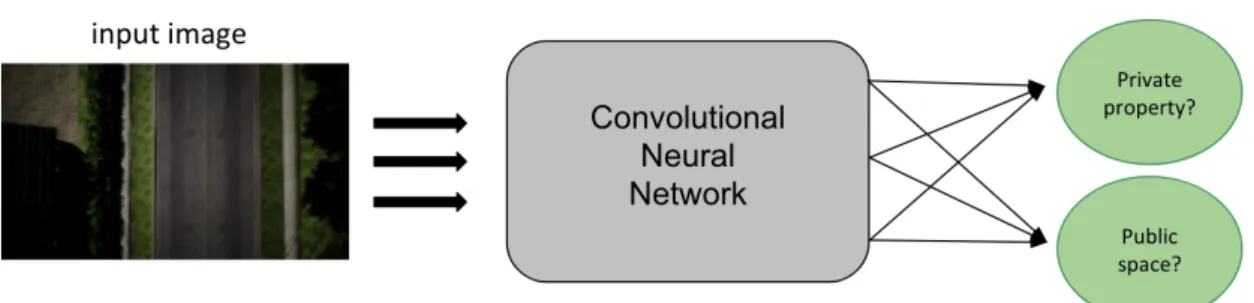
Convolutional neural networks (CNN) are typically used in supervised learning, where the network applies a label to an image, basically by ranking the labels that best fit the image in terms of their probabilities. A good example is shown in Figure 3.1, identifying whether an aerial image obtained by a drone is likely to be of a private property or not [GM18], just for the infinite number of possibilities it holds.

3.1 Neural networks in RL 17

Figure 3.1: Example of a binary image classification problem using a convolutional neural network in order to decide whether a drone is flying over a private propierty or the public space.

In the case of reinforcement learning, the convolutional neural network used in supervised learning to label images, is used to rank the possible actions of a given state. In other words, it helps to approximate the agentpolicypt, mapping states to the best action, taking into

accountQ(s,a), that as we stated before, maps state-action pairs to the highest combination

of immediate rewards with all future rewards that might be gathered by later actions in the trajectory. With the expected rewards assigned, the Q function will basically select (when acting greedy) the state-action pair with the highest Q value. A basic approach is what Figure 3.2 represents.

Figure 3.2: Example of an agent that following an optimal policy maps each state (represented by an image) into two possible actions, moving forward or rotating.

18 Deep reinforcement learning The main difference relies on how the neural network adjusts its weights. In supervised learning, the problem begins with the knowledge of the labels that the neural network will try to predict. The mapping is directly done from images to labels taking into account the backpropagation error of the network. For the case of reinforcement learning, neural network coefficients will be initialized stochastically, and using feedback from the environment the neural net will use the difference between its expected reward and the obtained reward to adjust its weights and improve the state-action knowledge.

Noticeably, reinforcement learning problems set up more restrictions than a simple supervised learning one, basically because it relies on the environment to send a scalar number in response to each action carried by the agent. This seems obvious, as it is how reinforcement learning works. But the rewards are delayed and affected by unknown variables introducing noise to the feedback loop. The neural network will need to adapt to a more complex expression of the Q function. It will take into account not only the immediate rewards produced by an action, but also the delayed rewards returned several time steeps later in the sequence.

3.2 Deep Q-Network

Risen from the inspiration of DeepMind recent research publications, we used Keras [C+_15],

as it will be later explained along Chapter 4. in order to build a similar neural network architecture for our project. As stated by DeepMind, the overall goal is to use a deep convolutional neural network to approximate the optimal action-value function

Q_p(s,a) =max

p E[rt+grt+1+g

2_r

t+2+...|st=s,at=a,p] (3.1)

which represents the maximum of the sum of rewardsrt discounted byg at each time-step

t, achievable by a behaviour policyµ =P(a_|s), after making an observation (s) and taking

an action (a) as previously explained in the Q-learning section.

The release of the DQN (Deep Q-Network) paper by DeepMind [MKS+_{15] noticeably}

changed Q-learning introducing a novel variant with two key ideas.

The first idea was using an iterative update that adjusted the action-values (Q) towards target values (gmaxaQ(st+1,a)) that were only periodically updated, thereby reducing

corre-lations with the target.

The second one was using a biologically inspired mechanism named experience replay that randomizes the data removing correlations in the observations of states and enhancing data distribution, with a higher-level demonstration and explanation by previous research in [MMO95], [OPBDC10] and [Lin93]. The use of the experience replay encourages the

3.2 Deep Q-Network 19

choice of an off-policy type of learning, such as Q-learning, because if not, past experiences would have been obtained following a different policy from the current one. Two huge advances can be taken out from this, one is that each training batch consists of samples of experience obtained randomly from the stored samples and current experience, so temporal correlation is clearly avoided. The other one is that each step in the agent’s experience can be used in many weight updates, so a significant gain in efficency is obtained in learning from the environment.

The whole process consists in parameterizing an approximate value functionQ(s,a;qi)

using the CNN shown in 3.3, in whichqiare the weights of the Q-network at iterationi. For

the experience replay, agent’s experienceset(tt,at,rt+1,st+1)are stored at each time-steptin

the replay memoryD{e1, . . . ,eN}, whereNsets the limit of entries, with the possibility of

replacing older experiences for new ones when the limit of the memory is reached.

The standard Q-learning update for network parametersq after taking actionAt in state

St and observing the immediate rewardRt+1and resulting stateSt+1is

q =qt+a[yQt Q(St,At;qt)]—qtQ(St,At;qt), (3.2)

wherey_tQis the estimated return and is defined as Q-target:

y_tQ=Rt+1+gmax_a Q(St+1,a;q) (3.3)

This update resembles stochastic gradient descent, updating the current valueQ(St,At;qt)

over the TD-error towards a target valuey_tQ.

As exposed in [MKS+_{13] and [MKS}+_{15] the agent was evaluated into the Atari 2600}

platform. It offered a diverse array of tasks designed to be difficult and engaging for human players. Using a reinforcement learning feedback and stochastic gradient descent in a stable manner together with large neural networks incredibly outperformed the best existing reinforcement learning methods on 43 out of the 49 games without incorporating any additional prior knowledge.

The trained agents were compared to professional human testers scores playing under controlled conditions. The publication showed that the DQN agent achieved more than 75% of the human score on more than half of the games (29 out of 49).

To comprehend and summarize all the concepts, a practical overview is useful. Taking into account DRL is living through a massive research hot topic and every week new publications appear to change and enhance previous methods, displaying clearly the main ideas behind [MKS+_{13] and [MKS}+_{15] will help new readers.}

20 Deep reinforcement learning

Figure 3.3: CNN architecture for DeepMind DQN playing Atari games [MKS+_{15]. The}

input to the neural network consists of an 84 X 84 X 4, followed by three convolutional layers and two fully connected layers with a single output for each valid action. Each hidden layer is followed by a rectifier nonlinearity (ReLU)

• End-to-end learning values ofQ(s,a)from pixelss

• Input statesis stack of raw pixels from last 4 frames • Output isQ(s,a)for 18 joystick/button positions

• Reward is change in score for that step • Take actionataccording toe-greedy policy

• Store transition(st,at,rt+1,st+1)in replay memoryD

• Sample random mini-batch of transitions(s,a,r,s0)from_D

• Using variant of stochastic gradient descent

• Compute Q-learning targets w.r.t. old, fixed parametersw

• Optimise MSE between Q-network and Q-learning targets

Li(wi) =Es,a,r,s0_⇠Di[(r+gmax

a0 Q(s

0_,a0_;w

3.2 Deep Q-Network 21

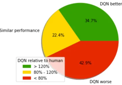
With a little more detail, our Figure 3.4 shows the published performance in games among three main blocks: Games in which DQN achieves a better performance than the human tester score, the ones in which a similar performance (between 80-120%) is obtained, and the rest, which is the biggest group, in which the human tester achieves a better score in the games than the DQN algorithm. After all, the assumption extracted from the publication that "the DQN agent achieved more than 75% of the human score on more than half of the games (29 out of 49)" is true, but when paying attention to the real values segmentation, human testers clearly obtain a better overall performance.

Figure 3.4: Pie chart exposing a comparative analysis on game performance for DQN and human testers.

The following graphs in Figure 3.5 exhibits the performance results of 10 games out of the total 49. These games are chosen as the best and the worst five for DQN relative to the human scores.

22 Deep reinforcement learning

(a)The percentage shows the human performance

compared to the DQN best five played games (b)

The percentage shows the DQN performance compared to the human best five played games

Figure 3.5: Colors are chosen relative to green seen as a better performance for DQN and red seen as a worse performance for DQN.

3.3 Double DQN

Using the Q-learning algorithm results in a positive bias by definition due to the maximum of the estimates is used as an estimate of the maximum of the true values, making it likely to select overestimated values using a greedy policy as the target policy. From 3.3 one may realize it uses the same samples both to select the maximizing action and to estimate its value, which results in a slower convergence to the optimal policy [SB98]. The idea proposed in [Has10] and named asDouble Q-learningis basically based in decoupling action selection from evaluation.

Two action-value functionsQ1andQ2are learned by assigning each experience randomly

to update one of the two function with the two sets of weights,q andq0_{in Double Q-Learning,}

one set of weights is used to determine the greedy policy and the other its value. First, the authors rewrite equation 3.3 as

yQ_t =Rt+1+gQ(St+1,argmax

a Q(St+1,a;qt);qt). (3.5)

And the two Double Q-learning targets can then be written as

yDoubleQ1 t =Rt+1+gQ2(St+1,argmax a Q1(St+1,a;qt);q 0 t) and (3.6) yDoubleQ2 t =Rt+1+gQ1(St+1,argmax a Q2(St+1,a;q 0 t);qt).. (3.7)

3.3 Double DQN 23

As referenced,Q1is used to determine the maximizing actionA⇤=argmaxaQ1(a)and

Q2is used to provide the estimate of its value withQ2(A⇤) =Q2(argmaxaQ1(a))shown in

(3.6). The second set of weights can be updated symmetrically by switching the roles ofq

andq0_{into (3.7), achieving unbiased estimates.}

As only one estimate is updated per step in a random selection, but two estimates are learned, it doubles the memory requirements but not the computational effort made at each step. The Double Q-learning was extended for the DQN-algorithm in [VHGS16]. Furthermore, the DQN-algorithm provides with the target networkq a natural candidate for the second value function, without having to introduce additional networks. TheDouble DQNalgorithm remains the same as the original DQN-algorithm, except replacing the target

yDQN explained in [Ker18] due to the limited space with

yDoubleDQN1 t =Rt+1+gQ2(St+1,argmax a Q1(St+1,a;qt);qt ) resp. (3.8) yDoubleDQN2 t =Rt+1+gQ1(St+1,argmax a Q2(St+1,a;qt );qt), (3.9)

where the weights of the second networkq0 _{of double Q-learning in (3.6) and (3.7)}

are replaced with the weights of the target network q , performing the update to target network as in neural fitted Q-iteration introduced before. This project revolves around the two mentioned algorithms, DQN, and Double DQN (DDQN).

Chapter 4

Materials and methods

The first approach for our drone framework was carried in [Ker18] and showed incredibly great results. The best performing Double DQN-agent obtained an 80% success rate during evaluation. While the overall performance remained below the human-level of comparison, potential improvements were identified on several aspects that could lead to even higher reliability and a superhuman performance.

Like in any other reinforcement learning proposal, one must set some boundaries and define a given problem and a certain solution. Our approach is to train an autonomous UAV to reach a goal in the minimum amount of time without colliding with any obstacle. This can be extended to reaching multiple goals in a single flight or even more complex things that will be introduced later. For a broad knowledge of how everything works, each improvement to the baseline is summarized and exposed in a simplified way.

The development of this project has been possible due to recent progress in open-source libraries and public repository collaborations. This chapter presents which resources have been used. Obviously, nowadays there is a vastly amount of competence between frameworks and libraries, ergo there are different ways of approaching the same problem and are continu-ously being updated. For every project requirements and resources there are more efficient solutions than others, and this always has to be analyzed first. Building a unique framework for DRL methods for UAVs, one of the initial motivations of this project is a difficult task to release and maintain. In this chapter we will analyze the tools used in order to build up our framework and its integration, together with the implementation and improvement from the previous baseline. The code is publicly available in Github and open to external contributions. Excluding code for graphs, front-end development and miscellaneous, everything can be found in the same remote repository: https://github.com/guillem74/DRLDBackEnd

4.1 Tools 25

4.1 Tools

All the development in this project has been built with Python, motivated by the great data science and machine learning community and both framework’s availability and excellence. Python is also a great and easy language for beginners, being simple to code and holding a fast learning curve for software developers when jumping from another language.

Figure 4.1: Overview of agent-environment interaction using our DRLD BackEnd

In order to visualize an scheme of the whole system, we provide Figure 4.1 which stands the same as in the first version of the framework. Every component will be explained below but one can rapidly figure out how the interaction is built up. As an overview, AirSim

provides us with a solid UAVs simulator,OpenAI Gymbrings us a toolkit for building up reinforcement learning algorithms andkeras-rlacts as a library that allows us to implement deep reinforcement learning algorithms. The first version of our framework was named

AirGym-v0but we consider it as deprecated due to recent updates in AirSim APIs. In addition, the idea of a name that includes a reference to OpenAI Gym framework limits us when willing to merge into a version that supports multiple frameworks.

4.1.1 AirSim

AirSim [SDLK17] is an open source simulator of vehicles based on Unreal Engine (UE4) from Microsoft AI and Research. AirSim profits from the really good rendering techniques of UE4 brought by the game industry [KG13] bringing strong graphic features and ultra realistic rendering capabilities, see Figure 4.3 as an example. Without the need of being a professional, you can modify existing environments or build your own by implementing objects, blueprints and behaviours in C++, apart from having the access to existing environments.

26 Materials and methods There are two main motivations for choosing AirSim. The first is their quadcopter realistic features, allowing simulations of existing UAVs such as Parrot AR Drone 2.0 [Par12] inside the game engine with at the same time supporting hardware-in-loop with popular flight controllers such as PX4 for physically and visually realistic simulations. And the other one is that it is basically built up for programmatic control, it exposes APIs so the user is able to interact with vehicle in the simulation programmatically. You can use these APIs to retrieve images, get state, control the vehicle and so on. The APIs are exposed through RPC and accessible via variety of languages including C++, Python, C-sharp and Java. The most important API features for our project are performing UAV complex movements and posing cameras to collect images such as depth, disparity, surface normals or object segmentation. These features make AirSim the strongest option within drone simulators. AirSim is a platform under development and with a large community which really helps it to grow, inserting pull requests into AirSim’s public repository or opening issues when errors or improvements come to light.

4.1.2 OpenAI Gym

OpenAI Gym [BCP+_{16] is a standard framework for setting up reinforcement learning tasks.}

Gym is a Python toolkit for developing and comparing reinforcement learning algorithms, making no assumptions about the agent’s structure in any problem.

Gym aims to help RL research by two main factors:

• The need for better benchmarks: While in supervised learning, progress has been driven by large labeled datasets like Imagenet [DDS+_{09], in RL there is the}

need to collect large and diverse environments. However, the existing open-source collections of RL environments don’t have enough variety, and they are often difficult to even set up and use.

• Lack of standardization of environments used in publications: Differ-ences in problem definition, such as the reward function or the set of actions make RL problems complicated to code. This issue makes it difficult to reproduce published research and compare results from different papers.

In other words, Gym lets you create your own environment or use one available. By environment, we do not mean the simulator or game, it means the programmable interaction with it. In Gym you are able to define and obtain, at each time-step, the information needed to piece together and later feed the RL algorithm. The developer has to set up anEnvclass which defines how each step is accounted and enables the reset function. The step function

4.2 Checkpoints 27

returns the substantial information for the RL algorithm, meaning the state, the reward, the action taken, if the task is in its terminal state and some extra information. A more detailed explanation can be found athttps://gym.openai.com/docs/.

4.1.3 Keras-rl

Keras-rl [Pla16] implements state-of-the-art deep reinforcement learning algorithms in Python and seamlessly integrates with the deep learning library Keras [C+_{15], working}

also with OpenAi Gym, making it all more simple. Keras has been gaining space in the Deep Learning industry, being a high-level neural networks API for easy and fast prototyping and the ability to run seamlessly on CPU or GPU (although little things can be done with CPU nowadays). Researchers in both convolutional and recurrent networks prefer to use Keras instead of other low level library, thanks to its modularity and extensibility. For this project, Keras core will be using Tensorflow as the back-end library, but Keras-rl has the possibility to use also Theano or even CNTK.

Keras-rl is built according to the developer needs, giving the ability to define own callbacks and metrics. More in depth, it also provides an easy access to implementing or redefining own algorithms by simply extending some abstract classes. Documentation can be found athttp://keras-rl.readthedocs.io/en/latest/. As we stated in the last section, this project revolves around two algorithm extensions, DQN and Double DQN (DDQN), which are going to be the used and implemented branches in Keras-rl. If you take this recommendation, try out and implement also Deep Determinisic Policy Gradient (DDPG) [LHP+_{15] or Deep}

SARSA [MBM+_{16], two upcoming and strong algorithms in reinforcement learning.}

4.2 Checkpoints

The main issue from previous work was found to be that during training phase, the random actions taken by the behavior policy created oscillations in the obtained reward. Additionally, a lot of executions were aborted before finishing training and that produced a huge lost on time. An improvement was required in order to train the algorithm for a long period of time and obtain the best possible results achieving high efficiency. Motivated by the inconsistencies of the AirSim simulator, which had been under development as this thesis was conducted, a contribution was demanded in order to keep training phases safe.

A pull request was submitted to keras-rl [Pla16], and it turned into a successfully approved contribution to the open-source library. The code developed was able to check at the end of

28 Materials and methods each episode whether the agent achieved a better performance than before, and if desired, write the neural network weights into disk before ending the whole training phase.

Checkpoints clearly solved two main problems, which were introduced at the end of the thesis carried in [Ker18]. On the one hand, and the most obvious, was being able to save the current best or even not best, if configured, weights when training was intentionally or accidentally stopped at a certain time-step. On the other hand, and as it will be shown later on, training curves exposed previously to this improvement, clearly exhibited a tendency of not finishing with the best agent’s reward efficiency, which induced a worse behavior in testing mode. We provide more information in our recent accepted publication on Digital Avionics Systems Conference (DASC)here.

4.3 Agent-environment design

This section will explain the development in each field of the reinforcement learning task separately. It clearly focuses on the environment and the agent features separately, including the available actions, the reward function and the definition of the state.

4.3.1 The environment

The new environment is part of the AirSim v1.1.8 release for Windows binaries build from the Modular Neighborhood Pack in Unreal Engine. The map creates an entire real-world systematic. It includes an entire residential zone, parks with animated winds on trees and a broad range of streets originating a real neighborhood.

(a)Inside environment and front view of the

quadcopter (b)Three-dimensional view over the area

Figure 4.2: AirSim Neighborhood environment views.

Unlike the blocks environment introduced in the baseline, this new environment generate a new issue, related to dimensions. Although not all the environment is captured from

4.3 Agent-environment design 29

4.2b, because it involves also more green zones, which are not so important for us, this new map covers an area of approximately 770⇥770 meters, 17 times bigger than the columns

environment. This is an enhancement, approaching the simulation to reality, but also has a drawback, taking into account training times. A solution for that problem will be presented in the following subsection.

Data and variables used for the deep reinforcement learning task are presented in Table 4.1. Three new blocks have been introduced, which are going to be discussed from now on.

Table 4.1:Data fetched from the simulation environment at every time-step.

Data Meaning

px, py, pz agent’s global x, y andz position

dx,dy,dt agent’s x, y and total distances to goal

dgxmin,dgxmax,dgymin,dgymax agent’s distances to geo-fence limits

y yaw angle relative to current orientation

DepthImage depth image in camera plan (144⇥256)

arrived boolean landing info

collided boolean collision info

Geo-fencing

Geo-fencing is known as a method of defining a virtual barrier on a real geographical location. Restricting the flight zone of a UAV has been useful in many cases. Another classic examples are the use of targeting citizens to promote proximity marketing or to send warnings of safety alerts via SMS.

In aerial systems, geo-fencing has been widely used for many approaches. In the area of UAVs, an expert in GPS security [Hum15] and a politician [Sch15b] suggested in 2015 that government regulators should encourage drone manufacturers to build geo-fencing constraints into UAV navigation systems that would override the commands of any operator, preventing the device from flying into protected airspace.

For the case of our simulations, the geo-fencing concept is the most suitable approxima-tion to increase realism. Also, programming a parametrizable geo-fence inside the AirSim simulator [SDLK17] prevents the agent from exploring scenes inside the environment that are not useful for accomplishing a certain task, resulting in a decrease in training time.

30 Materials and methods

(a)Possible geo-fencing for a targeted zone (b)Top view perspective

Figure 4.3: Geo-fencing limits for our quadcopter.

The idea evolves around the possibility of defining six different fences, two for longitude, two more for latitude and the last ones for altitude at the beginning of each training. Therefore, by adapting both state information and the reward function, the drone has to learn the concept of geo-fencing as another element of the environment; being rewarded negatively when trying to transgress it, and further creating the sufficient knowledge for avoiding it.

Landing

Approximating the simulation towards reality is not a trivial task. Our interaction with the environment needs to be adjusted to real physical dynamics. Drone flights include a takeoff period, the flights itself and a landing period.

Within this approach, the quadcopter takes off to a certain altitude and it remains constant until it reaches the goal coordinates. Nonetheless, it has to fetch altitude positionzat every time-step to control, maintain and adjust it when the goal is reached. Upon arriving to the destination, the altitude is slowly diminished until the quadcopter totally lands on the surface, achieving a controlled and stable movement.

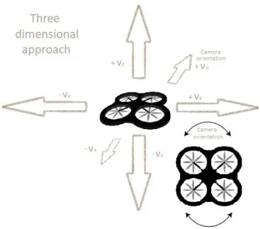
Even though a three dimensional dynamism is implemented at this stage, a slightly nearer to three dimension control version is acquired. Recent progress in drones has lead to include the possibility of sending commands from ground-control stations in order to perform discrete actions, such as taking off, landing, and rotating or moving forward at a fixed altitude, which is what we aim to replicate with an autonomous version of it. Obviously, a three dimensional control would imply a fully transferable to real-world format.

4.3 Agent-environment design 31 Multiple destinations

Expressed at the beginning of the project, one of the main problems of reinforcement learning and robotics in general is environment exploration. Gathering the sufficient knowledge of its surroundings, an agent could be able to take optimal decisions at any given moment.

Nonetheless, general artificial intelligence is not yet achieved and there are many mathe-matical restrictions on it. On the other side, there are some things which actually enhance the fact of learning more general concepts, in order to later extrapolate from it.

At this project we have already introduced some concepts that boost exploratory issues within deep q-learning. Some of them were using ae annealed policy or modifying the experience replay size. Other potentially important contributions to general intelligence will be explained at the 5.4.2 subsection, which contains already studied and researched areas but not yet well implemented for this project.

In order to gain more data for the agent, we came up with a more elaborated type of training. While the origin for the UAV was always the same, the destination of the goal changed. The reason of not changing the origin was purely AirSim restrictions. Before the new 1.2 release, thrown the 21st of June, the only way of changing the origin of a vehicle was via reading a static JSON at the execution of the binary. So, there was now way to dynamically read it during the same training. Now, thanks to open-source suggestions, Microsoft developers changed it to API calls, making it easier and more accessible.

Therefore, the agent is capable to learn different tasks with different goals within the same training process. This focused more on a general knowledge, rather than the spe-cific accomplishment of a goal, which is basically what a more broad intelligence tries to address. The later analyzed metrics comprise the training to four different destinations, randomly sampled at the beginning of each different episode, which made the task less repetitive and more complex. The chosen destination at each episode is one of the following,

[(137, 48),(59, 15),( 62, 7),(123,77)], respectively as always to theNeighborhood

map. Noticeably, this change affects the geofencing limits, which were adapted in the code. The destinations were chosen to be representative of a real possible destination case.

4.3.2 Actions

In the first baseline, actions were limited to three different ones, going straight, and per-forming a right yawor left yawwith different angles to be able to follow more possible directions.

Although we use this set of actions for various testing and results examples, we drastically changed this initial approach for a more realistic one.