Task Scheduling for Mobile Robots Using Interval Algebra
Lenka Mudrova
1and Nick Hawes
1Abstract— We present a novel task scheduling algorithm for use on mobile robots in real environments. The scheduling prob-lem is formalised as mixed integer program, which is a standard approach in the scheduling community. Our contribution is the use of Allen’s interval algebra to prune the search to be performed by the mixed integer program. This significantly speeds up the algorithm. The proposed algorithm has been used on several mobile robots in long-term autonomy scenarios, where it schedules large sets containing a variety of tasks. The proposed algorithm outperforms the state of the art by at least one order of magnitude on both these real tasks and synthetic datasets.
I. INTRODUCTION
Our lives are largely based on schedules, with our be-haviour being strongly determined bytime-dependent tasks, e.g. we need to be at work, at meetings, at the airport to take our plane for holiday, at specific times. If we are to use autonomous service robots to assist us in our lives, such a robot must respect such time constraints. For example, imagine a user giving the task “Come to my office at 10:00 and collect a letter” to a robot. The task might not be valid after this time, and if the robot fails to respect this time constraint the users would have to do it themselves.
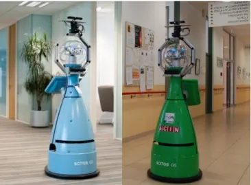
As part of STRANDS project1, we have deployed robots in care and security scenarios, where people’s health and property are involved (see Fig. 1). In the care scenario, we cooperated with “Haus der Barmherzigkeit” – a facility for elderly people in Austria. Our robot performed 1985 tasks during 14 days of deployment, including navigating to the chapel or game room, and regularly checking the emergency exits for obstructions. In the security scenario, we cooperated with G4S. In one of their buildings the robot performed 9631985 tasks during 16 days. For example, our robot created 3D maps of rooms at scheduled times, checked the position of fire extinguishers, and searched for objects on desks. In such scenarios, tasks have strict deadlines and their violation could cause significant risks to the property and health of users.
A. Scheduling
Before providing a formal definition of our scheduling problem (see Sec. II), we clarify the terms we use, in order to be able to relate existing work with ours. In the literature, the term “scheduling” is often misused to describe just the
ordering of tasks or to express the fact that a task has
time properties(whether or not their execution is organised
1School of Computer Science, University of Birmingham, B15 2TT
Birmingham, The United Kingdom [email protected], [email protected]
1http://strands-project.eu
with reference to these properties). For example, ordering appeared (as scheduling) for the robot RHINO [1] and expressing time constraints appeared (again as scheduling) in the robot MINERVA [2] extending work from [3]. In our work we tackle the pure scheduling problem: each task must be assigned a time instant when its execution starts, while time constraints (e.g. deadlines) are not violated.
The termstask, activityandactionare also used differently in literature. In this paper, atask has the time properties:
• release dater(the earliest time instant when a task can start),
• deadline d,
• processing time p (how many time units a task con-sumes),
• start time of executions, • end time of executione.
We refer to these properties for a specific taskj by adding a subscript, e.g.rj is the release date for taskj.
A task is also associated with anactivity to perform, for example “check the fire extinguisher”. An activity contains differentactions, for example “Go to loc5”, “take a picture with robot’s camera”, “run object recognition” etc. Actions are indivisible, they can be used in any combination to create a new activity for a new task. In this work we only consider scheduling at the level of tasks, and assume that the actions which comprise an activity are fixed.
B. Scheduler requirements
We set the following requirements for a scheduler based on the demands of our user scenarios. A scheduling problem
is static (the set of tasks is known beforehand) [4], but when a new task occurs a new scheduling problem is created to replace the previous one. The speed of the algorithm is generally more important than optimality of a final schedule, as we prefer the robot to act within a reasonable time limit when given a task. In this paper, we set this limit to three minutes as an upper limit for people’s patience. The daily routines provided to our robots require them to be able to schedule 200 tasks. The deadlines and release dates of these tasks must be respected. Tasks are performed in different locations, thus a robot needs to travel between them. A schedule must therefore take travel time into account.
C. Related Work
Two main approaches to solve the specified scheduling problem exist: pure schedulingandtemporal planning. The boundary between these approaches is not clear [5]. The scope of the following literature review is restricted to a specific domain: a mobile robot performing tasks required by a user.
1) Temporal planning: There are several ongoing projects using temporal planning. The social robot Tangy schedules multi-user activities, while considering users’ schedules [6]. It uses the OPTIC temporal planner [7] that uses PDDL to specify a set of tasks, and users’ schedules are represented as Timed Initial Literals (TILs) [8]. In [9], indoor and outdoor robots cooperate in a senior residential facility. The specified problem contains causal, temporal, resource and information constraints and which are encoded as a configuration plan. None of aforementioned approaches take space constraints on objects into account. This is overcome in [10], where authors proposed a new spatial knowledge representation calculus ARA+.
Temporal planning techniques such as these offer expres-siveness for task description (including objects, locations, resources etc.). However, tasks are expressed as a conjunc-tion of their goals, which can produce a large search space for large problems, greatly slowing down the search for a schedule. Since our system is required to schedule a high number of tasks (up to 200), we decided to not use temporal planning.
2) Scheduling: Simple Temporal Networks (STNs) [11] and Mixed Integer Programming(MIP) are two techniques well-known in the scheduling community. STNs are used in a robot who monitors the activities of an elderly person [12]. The activities and their time relations are prepared by a carer beforehand and they are mapped to a temporal constraint language in O-Oscar architecture [13], which is built on top of a STN. MIP is used in a scheduler proposed by Coltin et. al [14] for the CoBots project [15], where multiple indoor robots operate in an office building. Since this scheduler has good robustness, it was also used in multi-robot systems solving the Collection and Delivery Problem with Transfer
(CDP-T) [16]. Coltin et. al’s work has been used extensively in experiments in real environments and it reliably solves scheduling problems in a scenario similar to ours – fulfilling users’ tasks in large office buildings. It also satisfies our
requirements for release dates, deadlines and it takes into account travel times between locations.
In conclusion, scheduling is a suitable technique to execute large sets of tasks, which have predefined activities. Due to the match between Coltin’s et. al’s work and our own requirements, we have chosen to base our own research on their approach.
II. PROBLEM DEFINITION
Following the standard terminology in [17] a scheduling problem in our domain can be specified as:
1|r, settingjk, d|
X
C , (1)
where
• 1 refers to scheduling for a single robot. • rrestricts that tasks haverelease dates.
• settingjkstands forsetting timebetween processing of
taskj and taskk.
• drefers to fact that deadlines must be respected. • PC is an optimisation criterion referred astotal
com-pletion time.
The specified problem can be solved by a scheduler, which receives an input set of tasks S = {j, k, l, . . .} and finds time instants{sj, sk, sl, . . .}, when the execution of those
tasks must be started. As a single robot is assumed, the scheduler must ensure that no tasks overlap. Therefore, it finds such an ordering of the tasks in series, which minimises the chosen optimisation criterion. Moreover, a scheduler must respect the following properties of a task. The execution of the taskjcan start atrelease daterj or later, and it must
end before or atdeadlinedj. Thus, thetime windowhrj, dji
is defined for each task. The activity for task j lasts from start time instant sj to end time instant ej and consumes pj units of time. pj is referred as the processing time. The
relation issj+pj=ej. Following equation must hold: sj, ej ∈ hrj, dji. (2)
A robot starts to execute the task at location ls
j and ends
at locationle
j. The setting time settingjk =time(lej, lks)is
how long a robot travels from end locationle
j of taskjto the
start location ls
k of taskk. To obtain this travel time when
using a real robot, we use a learning approach [18]. Note that a robot may take a different amount of time to travel from le
j tolsk than in the reverse direction, due to environmental
constraints.
III. PRUNING SCHEDULER USING INTERVAL ALGEBRA
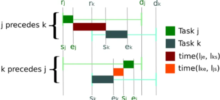
The aforementioned scheduling problem is solved by our proposed algorithm. The algorithm defines a set of con-straints for each task. These concon-straints ensure that all the time properties of the tasks are fulfilled and that no two tasks overlap. These constraints are solved using MIP to find the start instant for each task. In general, two orderings are possible for a pair of tasksj, k, either “j precedes k” or “k precedesj” (see Fig. 2). Solving the task constraints selects one of these orderings (satisfying both the task constraints
Fig. 2. Visualisation of two possible situations for taskj andk, which has overlapping time windows. Tasks are same in both situations, but the travel time differs. In this case, both situations are valid, as both tasks can be finished before their deadlines.
and the global optimisation criteria). Whilst expressing a scheduling problem as a set of constraints is a standard approach in the scheduling community, our contribution extends this through the use ofAllen’s interval algebra[19] to pre-select one of the possible orderings for each pair of tasks. This local optimisation greatly reduces the effort required by the constraint solver, but it does so at the cost of pruning possible solutions from the search space (losing both optimality and in some cases completeness). Our algorithm works as follows:
A) Every possible pair of tasks from the set is analysed. B) Allen’s interval algebra is used to prune possible
ordering for each pair.
C) The constraints are specified for chosen ordering. Step C) is based on Coltin’s et al.’s work [14]. The other steps represent the novel elements of our algorithm.
A. Analysis a Pair of Tasks
Having a pair of tasks j and k, four situations σ might occur:
• only “j precedesk” is possible (σ0);
• only “k precedesj” is possible (σ1);
• both situations are possible (σ2);
• neither are possible (σ3).
The σ for any pair of tasks depends on the relationship between their time windows (see Fig. 3). If the time windows do not overlap, then determining the ordering is simple. If the time windows do overlap use the following process to determine which situation holds.
First, we compute the parameter
εo= min(dj−rk, dk−rj).
ε0is positive if the time windows for tasksj andkoverlap.
Then, we test, which ordering –jprecedeskorkprecedesj – is possible. For each possible ordering, the maximal size of an interval where both tasks can fit isε1=dk−rj andε2= dj−rk, respectively. The following equations are tested:
ε1≥pj+time(lej, l s
k) +pk, (3)
ε2≥pk+time(lek, ljs) +pj. (4)
Then,
• σ0 occurs iff only Eq. (3) holds;
• σ1 occurs iff only Eq. (4) holds;
• σ2 occurs iff both equations hold;
• σ3 occurs iff neither equation holds. B. Pruning
When σ2 occurs, our algorithm picks one ordering
con-straint – j precedes k or kprecedes j – which it considers (locally) to be the best. This decision is made based on the thirteen possible relations of two intervals described by Allen’s interval algebra (see Fig. 3). For relations “overlaps”, “starts”, “finishes” the ordering constraint is chosen by testing the formula:
ε1> ε2.
If the formula is true, then orderingj precedesk is chosen and vice versa. This maximises the amount of time available for the tasks.
For the remaining interval relations (j during k,kduring jandjequalsk) the possible orderings are indistinguishable using the previous rule. Therefore, we choose the ordering constraint which locally minimises the global optimisation criterion PC. We calculate this for a pair of tasks as follows. First, we calculate the criterion P
C0, assuming
task j precedes task k. As no other tasks are considered, taskj can start as soon as possible, followed by task k:
sj = rj
sk = rj+pj+time(lej, l s k).
(5)
Then, the criterion for this ordering is: X
C0= (ej−rj)+(ek−rk) = (sj+pj−rj)+(sk+pk−rk).
This can be simplified using (5) to: X
C0=pj+rj+pj+time(lje, l s
k) +pk−rk. (6)
If the value ofsk in (5) is smaller than release daterk, then
its assignment in (5) is not possible. Instead, we setsk=rk
and the criteria is simplified to: X
C0=pj+pk. (7)
Next we calculate the criterionP
C1, assuming the
oppo-site ordering – taskkprecedes taskj. The criteria is similar
X C1= pk+rk+pk+time(lek, l s j) +pj−rj, when sj> rj,; pj+pk,when sj=rj; (8)
Finally we choose the ordering which produces the lowest P
Cvalue. If they are equal, then the order does not matter and we choose taskj to precedes taskk.
C. Scheduler’s Constraints
Following the results of pruning we build a scheduling problem by selectively applying the constraints proposed by Coltin et al.2. Following (2), the first constraint we use restricts the execution time of a task to its time window:
rj≤sj ∧ ej ≤dj. (9)
2Note that in comparison to [14] we usedto denote the latest time by which a task must end instead of the latest time when it task can start.
no constraint j precedes k k precedes j both j before k j meets k k before j k meets j j overlaps k j starts k k finishes j k overlaps j k starts j j finishes k j during k k during j j equals k
Fig. 3. Thirteen combination of Allen’s interval algebra
If ε0 ≤ 0, task j does not overlap with task k therefore
no additional constraints are needed for this pair of tasks. However, if ε0>0, we need to link the execution times sj
andskby a second constraint in order to ensure that the tasks
will not overlap. Coltin et al. treat all overlaps as situation σ2, but we distinguish between four situations:
• Forσ0, i.e.j ordered beforek: sj+pj+time(lje, l s
k)−sk≤0. (10)
• Forσ1, (the reverse ofσ0) the constraint is sk+pk+time(lek, l
s
j)−sj ≤0. (11)
• Forσ2, as both orderings are possible, both preceding
constraints (10, 11) should be added using a disjunction relation. It is this disjunction which enlarges the search space for the constraint solver and slows down the search for an optimal solution. However, all σ2 are
pruned to σ0 or σ1 by usingPC0 andPC1.
• Forσ3, there is a flaw in the input set and a schedule
is infeasible.
IV. EXPERIMENTS IN SIMULATION
We implemented both our proposed scheduler and the state-of-the-art scheduler from Coltin et al. [14] in C++, using SCIP 3.0.2 [20] to solve the constraints. Our code is available as a ROS package3.
Properties of Simulation
We have compared the two schedulers on synthetic task sets with the following properties. The input sets of tasks are always feasible. The processing time pj is generated
using uniform distribution between values2min and30min. The size of the time window hrj, dji is set to be ρ-times
bigger than the processing time pj, whenρis generated as
a random number with uniform distribution from interval h4,100i. Each set contains multiple groups of tasks, where all tasks within a single group have one type of Allen’s relation.
3https://github.com/strands-project/strands executive
ω 1 % 5 % 25 % 50 % 100 %
proposedt[s] 0.044 0.042 0.054 0.133 0.585 Coltin’st[s] 0.101 188.116 - -
-TABLE I
ALGORITHMS’DURATION DEPENDENT ON SIZE OF THE GROUP OF TASKS
n 10 20 100 200
proposedt[s] 0.003 0.006 0.097 0.585 Coltin’st[s] 33.238 196.012 -
-TABLE II
ALGORITHMS’DURATION DEPENDENT ON AMOUNT OF EQUAL TASKS
Hence, the release daterj and deadlinedj of each task are
set based on chosen Allen’s relation to other tasks within the group. The travel time between any two task locations is a constant. All tests were run on a Lenovo ThinkPad E-540 with Intel i74702MQ Processor (6MB Cache, 800 MHz).
A. Overlapping Time Windows
The performance of the two algorithms only differs signif-icantly whenσ2occurs (i.e. when our approach prunes away
possible solutions). To explore this case, ten sets containing 200 tasks each were generated. Each set consists of groups of tasks, where the tasks within the group overlap in a way such that the occurrence of situationσ2 is guaranteed,
but tasks from different groups do not overlap. The size of the group ω is set as a ratio to the overall amount of tasks. The results, presented in Table I, demonstrate that the proposed scheduler is faster than Coltin’s et. al on these problems. Moreover, increasing the group size leads to significantly higher computation times for Coltin’s et. al scheduler. This is mainly due to more possible combinations of task ordering, which the solver needs to take into account. We restrict ourselves to limit of three minutes to provide a solution. Thus, we did not run Coltin’s scheduler for all cases as the time increases exponentially. For the problems that both schedulers solved, the difference in optimality criteria between approaches is negligible.
B. Equal Time Windows
The situation when all tasks have similar time windows (i.e.ω= 100 %) is even more challenging than the previous situation. This is because there is no difference between time intervals, thus all possible orderings of tasks have the same optimum, but the solver is not aware of this. The results from both schedulers running on sets of equal tasks of increasing size are presented in Table II. A significant time difference between the approaches can be observed for a set containing only 10 tasks. Again, there is no difference in final optimisation criteria.
Dataset Amount of Sets Both failed Proposed failed Coltin’s failed HdB 606 103 24 33 G4S 358 14 2 3 TABLE III
COMPARISON OF CASES WHERE NO VALID SCHEDULE IS FOUND
V. EXPERIMENTS IN REAL ENVIRONMENTS As described in Section I, we ran a version of our sched-uler on long-running autonomous robots in the our project’s Haus der Barmherzigkeit care home scenario (abbreviated HdB) and G4S security scenario. We recorded all sets of tasks sent to the scheduler during these deployments and now compare the two schedulers on these real-world task sets. Many of the tasks in the sets were generated from a daily routine given to the robot and thus have large equal time windows (corresponding to morning, afternoon etc.). A smaller proportion of tasks were generated on-demand by users or other parts of the robot’s architecture. The nature of the routine-based tasks means that situationσ2often occurs. A. Existence of infeasible sets
In contrast to the simulated data, infeasible sets can exist in the data from the real environments. The proposed scheduler can only detect infeasible sets via σ3, but other infeasible
sets are possible which do not trigger this situation. Coltin’s scheduler can detect all infeasible sets, but only for the problems it can solve completely (which is limited by the size and nature of problems). Therefore, we cannot determine if any given set is feasible or not. Instead we compare if the schedulers fail to find a solution within the three minute limit. Table III presents counts of three possible outcomes:
• both schedulers fail;
• the proposed scheduler fails but Coltin et. al’s succeeds, (which occurs mainly for sets containing a small amount of tasks);
• Coltin’s et al.’s scheduler fails but the one proposed succeeds (which occurs mainly for sets containing a large amount of tasks).
B. Speed of the schedulers
The results in Figures 4 and 5 (for the G4S and HdB data, respectively) show that our proposed algorithm is sig-nificantly faster than the state-of-the-art as the size input set increases. It can be observed that the MIP problem specified by the proposed scheduler is completely solved within the three minute time limit for all sets. The word “completely” refers to the fact that the SCIP solver returns the optimum criterion for the specified MIP (which itself may be non-optimal for the problem). In contrast, MIP problem specified via Coltin et. al’s approach has a larger search space than ours and it cannot be completelysolved within the limit for most of the sets. However, the solver is still able to provide a solution when cut off as the limit is reached, but it cannot determine if this is the optimal one or not.
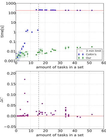
Fig. 4. Comparison of the schedulers in the G4S scenario
C. Quality of the schedules
We can determine which scheduler performs better on a task set by comparing the optimisation criteria of the resulting schedules. The absolute value of this criteria varies by task set, thus we compute the following normalised metric to provide a general comparison:
∆C= P Cp−PCc PC h , (12) where:
• PCpis the optimisation criterion of the result from the
proposed scheduler,
• PCc is the optimisation criterion of the result from
Coltin et. al’s scheduler,
• PCh is the highest (i.e. worst) possible optimisation
criterion for the input setS, which is computed as: X
Ch=
X
j∈S
(dj−pj−rj).
The property ∆C ∈ h−1.0,1.0i holds. This metric can be computed only for such sets when both algorithms have found a schedule. Negative values correspond to the fact that the proposed algorithm has found a better criterion than Coltin’s et al. and vice versa.
The ∆C values are displayed in lower graphs in Figures 4 and 5. In the graphs, sets to the left of the black dashed line are those with small amounts of tasks for which the
solver has found the optimal solution for both schedulers. Sets to the right of the line are those for which the solver has found some solution for Coltin’s approach and the optimal
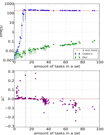
one for the proposed problem. In the G4S data (Fig. 4) the proposed scheduler found mostly worse criterion values, but the differences are negligible. In contrast, in the HdB data (Fig. 5) the proposed scheduler found mostly better criterion.
Fig. 5. Comparison of the schedulers in the HdB scenario
VI. CONCLUSIONS
In this paper we presented a novel fast scheduler for use on mobile robots. The main contribution of our work is the use of Allen’s interval algebra to prune possible solutions within the scheduler. Our experimental results have shown that the proposed scheduler is able to quickly solve task sets with large amounts of tasks, significantly outperforming a state-of-the-art designed for the same domain. In addition, the quality of the schedules found by our proposed approach in a limited time window is often higher (based on the optimisation criteria). This is despite the local nature of the optimisations in our approach potentially ruling out optimal and valid solutions. The proposed scheduler is open source and was integrated into two mobile robots which successfully performed 2948 tasks within 30 days in real-world application scenarios.
ACKNOWLEDGMENT
The research leading to these results has received funding from the European Union Seventh Framework Programme
(FP7/2007- 2013) under grant agreement No 600623, STRANDS.
REFERENCES
[1] M. Beetz and M. Bennewitz, “Planning, scheduling, and plan execu-tion for autonomous robot office couriers,” inIntegrating Planning, Scheduling and Execution in Dynamic and Uncertain Environments, volume Workshop Notes, 1998, pp. 98–02.
[2] S. Thrun, M. Bennewitz, W. Burgard, A. B. Cremers, F. Dellaert, D. Fox, D. Haehnel, C. Rosenberg, N. Roy, J. Schulte, and D. Schulz, “Minerva: A second-generation museum tour-guide robot,” in In Proceedings of IEEE International Conference on Robotics and Au-tomation (ICRA99, 1999.
[3] W. Burgard, A. B. Cremers, D. Fox, D. Haenel, G. Lakemeyer, D. Schulz, W. Steiner, and S. Thrun, “The Interactive Museum Tour-Guide Robot,” in Proc. of the Fifteenth National Conference on Artificial Intelligence (AAAI-98), 1998.
[4] J. Bidot, T. Vidal, P. Laborie, and J. C. Beck, “A theoretic and practical framework for scheduling in a stochastic environment.” Journal of Scheduling, vol. 12, no. 3, pp. 315–344, 2009.
[5] D. E. Smith, J. Frank, and A. K. J´onsson, “Bridging the gap between planning and scheduling.”KNOWLEDGE ENGINEERING REVIEW, vol. 15, p. 2000, 2000.
[6] W.-Y. G. Louie, T. Vaquero, G. Nejat, and J. C. Beck, “An autonomous assistive robot for planning, scheduling and facilitating multi-user activities,” inProceedings of the IEEE International Conference on Robotics and Automation (ICRA), 2014.
[7] J. Benton, A. J. Coles, and A. Coles, “Temporal planning with prefer-ences and time-dependent continuous costs.” inICAPS, L. McCluskey, B. Williams, J. R. Silva, and B. Bonet, Eds. AAAI, 2012. [8] A. E. Gerevini, P. Haslum, D. Long, A. Saetti, and Y. Dimopoulos,
“Deterministic planning in the fifth international planning competition: Pddl3 and experimental evaluation of the planners,”Artificial Intelli-gence, vol. 173, no. 5-6, pp. 619–668, Apr. 2009.
[9] M. D. Rocco, F. Pecora, and A. Saffiotti, “When robots are late: Configuration planning for multiple robots with dynamic goals.” in
IROS. IEEE, 2013, pp. 5915–5922.
[10] M. Mansouri and F. Pecora, “More knowledge on the table: planning with space, time and resources for robots,” inIn Proceedings of IEEE International Conference on Robotics and Automation (ICRA), 2014, pp. 647–654.
[11] R. Dechter, I. Meiri, and J. Pearl, “Temporal constraint networks,”
Artificial intelligence, vol. 49, no. 1, pp. 61–95, 1991.
[12] A. Cesta, G. Cortellessa, R. Rasconi, F. Pecora, M. Scopelliti, and L. Tiberio, “Monitoring elderly people with the robocare domestic en-vironment: Interaction synthesis and user evaluation.”Computational Intelligence, vol. 27, no. 1, pp. 60–82, 2011.
[13] A. Cesta, G. Cortellessa, A. Oddi, N. Policella, and A. Susi, “A constraint-based architecture for flexible support to activity schedul-ing,” inAI* IA 2001: Advances in Artificial Intelligence. Springer, 2001, pp. 369–381.
[14] B. Coltin, M. M. Veloso, and R. Ventura, “Dynamic user task schedul-ing for mobile robots.” inAutomated Action Planning for Autonomous Mobile Robots, ser. AAAI Workshops, vol. WS-11-09. AAAI, 2011. [15] M. M. Veloso, J. Biswas, B. Coltin, S. Rosenthal, T. Kollar, C. Mericli, M. Samadi, S. Brandao, and R. Ventura, “Cobots: Collaborative robots servicing multi-floor buildings.” inIROS. IEEE, 2012, pp. 5446–5447. [16] B. Coltin and M. Veloso, “Optimizing for transfers in a multi-vehicle
collection and delivery problem,” inProc. of DARS, 2012.
[17] M. L. Pinedo,Scheduling: Theory, Algorithms, and Systems, 4th ed. Springer Science+Business Media, 2012.
[18] B. Lacerda, D. Parker, and N. Hawes, “Optimal and dynamic planning for markov decision processes with co-safe ltl specifications,” inIROS. IEEE, 2014.
[19] J. F. Allen, “Maintaining knowledge about temporal intervals.” Com-munications of the ACM, vol. 26, no. 11, pp. 832–843, 1983. [20] T. Achterberg, “SCIP: Solving constraint integer programs,”
Math-ematical Programming Computation, vol. 1, no. 1, pp. 1–41, 2009, http://mpc.zib.de/index.php/MPC/article/view/4.