Using CSTPNs to model traffic control CPS

IET Software

Special Issue: Advances in Knowledge and Information Software

Management

Using CSTPNs to model traffic control CPS

Received on 30th May 2016 Revised 19th February 2017 Accepted on 22nd March 2017 E-First on 24th May 2017 doi: 10.1049/iet-sen.2016.0119 www.ietdl.org

Hongzhuan Zhao

_{, Dihua Sun}

, Hang Yue

_{, Min Zhao}

_{, Senlin Cheng}

1_{Key Laboratory of Cyber Physical Social Dependable Service Computation, Chongqing University, Chongqing, People's Republic of China} 2_{School Architecture and Transportation Engineering, Guilin University of Electronic Technology, Guilin, Guangxi, People's Republic of China} 3_{Johns Hopkins Healthcare LLC, Glen Burnie, MD, USA}

E-mail: [email protected]

Abstract: Transportation cyber-physical system (T-CPS) is a spatiotemporal discrete-continuous hybrid system. However, the hybrid T-CPSs have some analysis and modelling problems, especially the problems related to the spatiotemporal characteristics. Existing coloured Petri net approaches of traffic control cannot effectively analyse dynamic changes of cyber systems and physical entities in space and time. Moreover, some problems, related to the state space explosion and the large complex T-CPSs, have not been well solved. This study develops the innovative methods for T-CPS design and modelling via the development and application of coloured spatiotemporal Petri nets (CSTPNs). The proposed research ideas involve the CSTPN theory creation, the development of traffic intersection coordination control system using CSTPNs, the traffic simulation analysis and the implementation of T-CPS-based CSTPNs. The experimental results show that the new spatiotemporal theories and approaches of the traffic coordination control based on CSTPNs have excellent potentials to address the issues related to the spatiotemporal discrete-continuous characteristics of T-CPS. Moreover, these innovative methods with a good validity can be easily applied into practise for the development of T-CPS.

1 Introduction

Cyber-physical system (CPS), a hybrid system, is the combination of the PS and the cyber system. This hybrid system achieves a real-time monitor and control of the interconnection among the networks, the physics of the system and the computer components using different technologies (such as network, electrical communication, automatic control etc.). Intelligent transport system (ITS) consists of different transportation systems such as advanced traveller information system, advanced traffic management system, advanced transit system and so on [1]. T-CPS is a specific CPS for transportation applications, especially ITS, and the computing elements in the cyber system are coupled with the physical entities of the real world [2]. The authors in [3] described that transportation is a dynamic environment, consists of static roadways and moving objects (e.g. running vehicles and walking pedestrians). However, the spatiotemporal characteristics of traffic events cannot be readily identified from the cyber system, due to the support of insufficient spatiotemporal T-CPS theories. It is a significant problem in the analysis of traffic moving object events in T-CPS.

Fortunately, a Petri net (PN) is one of several mathematical modelling languages for the description of distributed systems. PNs are useful for the system study of information interrelation. As a kind of network, the token flow is used to describe the dynamics of a complex system. Also, PNs are a common modelling methodology for the integration of graphics and mathematics. This modelling methodology can clearly illustrate a system structure through visual graphs and easily analyse the system inherent characteristics using mathematical methods [4]. On the other hand, PNs can depict the entity relationship and the event interaction. More importantly, PNs can be used for the design of discrete event systems [5]. Girault and Valk [6] gave a PN model analysis for the development of design flows. Huang and Kirchner [7] used two different PNs to merge and create an integrated PN. In addition, PNs are very useful for the modelling and analysis of T-CPS. The research [8] described some specific hybrid PNs, and they are the combination of general PNs and continuous PNs; and Júlvez and Boel [9] developed a macroscopic model to describe the

behaviours of a traffic network using a continuous PN method. However, the traffic system analysis approaches are not accurate enough on the description of the spatiotemporal characteristics

concerning discrete-continuous hybrid T-CPS [10]. Febbraro et al.

[11] demonstrated a traffic model in a timed PN (TPN) framework, where the tokens cannot distinguish among different vehicles and their associated routes.

Given a multiform and multidimensional nature in transportation, it is hypothesised that a more efficient T-CPS is required to adequately address the spatial dimension into coloured TPNs (CTPNs). Also, it is hypothesised that using a combined spatiotemporal dimension is able to readily describe the dynamics of T-CPS. It can solve the state space explosion problem using coloured token set. More importantly, the use of coloured spatiotemporal PNs (CSTPNs)-based T-CPS can significantly optimise the performance of traffic intersection coordination control system (TICCS) and the real-time traffic control at intersection. The aim of this paper is to innovatively analyse and model T-CPS via the development and application of CSTPNs. The research content involves the CTPN theory description, the CSTPN theory creation, the TICCS improvement using CSTPNs and the experimental data analysis based on the typical traffic intersection.

Section 2 reviews the related literature. Section 3 depicts the CSTPN theory development based on the CTPN theory. Section 4 describes the CSTPN theory use on TICCS. The traffic simulation analysis is detailed in Section 5. Section 6 gives the implementation of the new theory. Finally, Section 7 gives a brief discussion and some concluding remarks.

2 Literature review

Some researchers discussed the development of spatiotemporal

hybrid systems for T-CPS analysis. Haghighi et al. [12] described

the spatiotemporal relationship using the definition of a spatial– temporal logic. This logic is a unification of a signal temporal logic and a tree spatial superposition logic, it can describe the change of high-level spatial patterns over time; Wu et al. [13] depicted the syntax and operational semantics and demonstrated the calculation methods of the operational and denotational semantics for the

development of the denotational semantics of spatial–temporal

consistency language; Mu et al. [14] developed a spatial–temporal

model to evaluate the impact concerning the large-scale deployment of plug-in electric vehicles on urban distribution networks; Chi et al. [15] created an improved Moving Objects in Networks Tree (MON-Tree), the index is divided into two levels

and the quad tree grid index at the top of the network; Kloog et al.

[16] developed a hybrid spatiotemporal model for the estimation of daily multi-year PM2.5 concentrations across northeastern USA using high-resolution aerosol optical depth data; moreover, the paper [17] used spatiotemporal automata to describe CPS.

Although the above research discussed some issues of spatiotemporal analysis, it was difficult for existing PN approaches to analyse the dynamic changes of cyber systems in time or describe the location changes of physical entities [18, 19]. The space explosion problem means the number of states or types of physical entities in a system is far greater than can be parallel handled in an established model which is mainly caused by the concurrent or interleaving semantics used to represent any sequences of possible actions. Owing to no difference among the different tokens of PNs, the analysis of the large complex systems often caused the state space explosion [20]. Huang and Chung [21] developed the TPNs with the support of time-series modelling to control the time plan of the physical entities, but the tokens of the TPNs cannot effectively analyse different entities and their associated properties.

To identify different physical entities, colours should be applied into the timed PNs, namely CTPNs. List and Cetin [22] used PNs to describe traffic signal control system and analyse the control model by P-invariants, and the model developed can guarantee the traffic operation safety rules. The research [21, 23] applied coloured PNs in traffic control system, but they ignored spatial, temporal or spatiotemporal characteristics of the traffic events. Although Silva and Recalde [24] and Dotoli et al. [25] discussed the hybrid models of discrete space and continuous state, they did not solve the analysis problems of the large complex T-CPSs. To optimise the PN model, Jűlvez and Boel [26] introduced the concept of coloured token transition related to CSTPNs.

The above literature review shows the previous studies have not well explored the spatiotemporal analysis methods for the development discrete-continuous hybrid T-CPS. Existing coloured PN approaches of traffic control cannot effectively analyse dynamic changes of cyber systems and physical entities in space and time. Moreover, some problems, related to the state space explosion and the large complex T-CPSs, have not been well solved. For the purpose of T-CPS optimisation, this study theorises CSTPN, improves TICCS using the new CSTPN theory, simulates the experimental data for the TICCS analysis and discusses the theory implementation.

3 Development of CSTPN theory

3.1 Coloured TPNs

The colour use in CTPNs is a useful tool to analyse the large complex T-CPSs. The CTPN is a bidirectional-digraph, and the basic formula of CTPNs (including seven tuples) is presented in (1) [27]

f_CTPN= (C, T, P, Wk(pi, tj), Pre, Pos, FT) (1)

where C is a colour function related to the elements in P ∪ T, and P ∪ T is a non-empty coloured set in the possible colour set Col. Given c_i= C(pi) is the number of possible coloured tokens in pi,

C maps the place p_i∈ P to the set of possible coloured token colours in (2)

C(pi) = {ai, 1, ai, 2, …, ai,cj} ⊆ Col (2)

C maps the transition tj∈ T to the possible coloured set of

events

C(tj) = {bj, 1, bj, 2, …, bj,cj} ⊆ Col, cj= C(tj) (3)

To keep the number of coloured tokens in a place, the weight function Wk(pi, tj) is defined as the inhibitor arc for the transition

connection of the place. The inhibitor arc is labelled as a ∈ N between p_i∈ P and t_j∈ T [namely W_k(pi, tj) = a]. Once there

were coloured tokens in p_i, the inhibitor arc would prevent the firing of t_j; _Pre(pi, tj) is a mapping from the event colour set of

p_i∈ P to the non-negative multi-sets N[C(pi)] over the colour set

of pi∈ P. Pre(pi, tj):C(tj) → N(C(pi)) is a matrix of non-negative

integers c_i× cj. Pre(pi, tj)(x, y) is equal to the weight of the arc

from the place p_i with the colour a_i,x to the transition t_j with the colour b_j,y.

Similar to the above Pre(pi, tj):C(tj) → N(C(pi)),

Pos(pi, tj):C(tj) → N(C(pi)) with tj∈ T and pi∈ P has the set of

directed arcs from T to P. _Pos(pi, tj) is a matrix of non-negative

integers ci× cj. Pos(pi, tj)(x, y) is equal to the weight of the arc

from the transition t_j with the colour b_j,y to the place p_i with the colour a_i,x. The marking m_i of p_i is described as a non-negative multi-set exceeding C(pi). The mapping mi:C(pi) → N(C(tj)) is

related to the possible coloured token colours in p_i. The marking M of CTPNs is described in (4), and the colour b_j,n enables the transition t_j∈ T at a marking M

M = m1, m2, …, mp T (4)

Given FT is a timing vector; t_j is the firing time of the transition; and FT_j specifies the deterministic duration of the firing of tj, it

satisfies the following two conditions: • m_i(x) ≥ Pre(pi, tj)(x, y), x = 1, 2, …, ci

where p_i∈ ∗ tj, ∗ tj= {pi∈ P:Pre(pi, tj) > 0, named pre-set of

t_j; and • _∑x = 1 ci _m i(x) ≤ Wk(pi, tj) where p_i∈ tj∗ , Wk(pi, tj) > 0, tj∗ = {pi∈ P:Pos(pi, tj) > 0}, named pos-set of t_j.

If the transition tj∈ T fires with respect to the colour bj,y, then it

would obtain a new marking m*, mi∗(x) = mi(x) + Pos(pi, tj)(x, y) −Pre(pi, tj)(x, y) with pi∈ P and x = 1, 2, …, ci.

The above analysis shows the PNs in CTPNs are discrete, but the continuous place changes of the physical entities in T-CPS have a requirement on the dynamical transition process. It is necessary to develop CSTPN to overcome the shortcoming of CTPNs.

3.2 Coloured STPNs

T-CPS is a special CPS for transportation applications. The analysis of temporal and spatial orders can address the issues related to the spatiotemporal characteristics of T-CPS. The temporal orders specify the relative marking sequences of the physical objects and line up a series of T-CPS events in time; and the spatial orders describe the directions, distances and priorities of the physical entities in space. Each traffic entity can be defined as a quintuple notation

TPE = (TPEid_{, TPE}attribute_{, TPE}behaviour_{, BA}mapping_{, CSTPNs) (5)}

where TPEid _{is the IDs of traffic physical entities; TPE}attribute _{is the}

attribute set of traffic physical entities; TPEbehaviour _{is the behaviour}

set of traffic physical entities; and _BAmapping is the mapping process from a TPE behaviour set to a TPE attribute set.

CSTPNs are used to depict the behaviours of traffic physical entities and the place transition processes of these entities using the coloured tokens. As an extension of CTPNs, CSTPNs can better model T-CPS, and have new types of places, functions, transitions and firing arcs. More importantly, CSTPNs offer the rules of storing, computing and transferring spatial information among the physical objects. The function of CSTPNs is given in (6)

f_CSTPN= (C < S > , T, P, Wk(pi, tj), Pre, Pos, FT) (6)

The spatial factor _{S = ⋃i}n_{= 1TPEi} is an entity abstraction set. Using the new storage and calculation methods of spatial information, CSTPNs can better describe the process of traffic cyber-physical

fusions and the dynamic interactions between TPEi and TPEj, and

these TPEs may have a change from the initial status to the target status. The use of this spatial factor, as an entity set, is better than the use of more parameters to describe the features of traffic physical entities and their dynamic interactions and status changes. Thus, it is the solution to the state space explosion problem.

Given that P_id is the identity name of state places (SPs),

Tokencolour is the coloured tokens set, Tokeninitial is the initial value

of the coloured tokens, SP can be presented as

SP(P_id, Token_colour, Token_initial). In terms of traffic event time records, traffic event positions and traffic information propagation in cyber systems, event transition (ET) is presented as

ET(Tran_id, Fung, Trancs), where Tranid is ET identity name; Fung is

a function to judge if the ET would happen or not; Trancs is a

function to describe ET process. About the temporal and spatial relationships between traffic state and traffic event. Arc of

Causation (AC) is presented as

AC(AC_id, Fun_arc, Token_number, Token_change), where AC_id is the AC identity name; Funarc is an arc function to describe the relationship

between places and transitions; Token_number is the number of

coloured migrated tokens; Token_change is the number of the

coloured changed tokens. Once the time stamp _FTj instantly

happens, the enabled transition t_j is ready to fire with respect to colour cj.

The above SP, ET and AC are the main parts of CSTPNs architecture for T-CPS modelling, as shown in Fig. 1.

CSTPNs for modelling T-CPS is defined in (7)

fT−CPS=< C(Pcoloured, Tcoloured), T, P, E, W, SR, D, R,

S_tat0 _> (7)

(see equation below) S_tat0 _{is given in (8)}

S_tat0 _{=< M}

0, Ca0, Ad0, Pt0, Ms0> (8) M0, Ca0, Ad0, Pt0and Ms0 denote initial markings, change attributes, addresses, playing time and firing states of the state No.0

in the propagation function, respectively. M_j, Caj, Adj, Ptjand Msj

denote these parameters of the state _{No . j} in the propagation function (see equation below) ‘0’ in Mj means that there is no

coloured token in a place and ‘1’ means there is one coloured token in a place. Ptj records the time spent by a coloured token. In the

firing state of every transition Msj, ‘true’ means a successful fired

transition and ‘false’ means a failed fired transition.

Once the coloured tokens arrive or leave, the states of these coloured tokens need to be updated. If a transition Tiis fired in the

state No . (j − 1) with a relative time τ, the firing rules of the modelled T-CPS are given in following equation:

M_j(P) =

Mj− 1(P) + W(Ti, P), for E(Ti, P) M_{j− 1}(P) − W(P, Ti), for E(Pi, T)

M_{j− 1}(P) + W(Ti, P) − W(P, Ti), for E(Pi, T) and E(Pi, T)

M_{j− 1}(P), otherwise

(9)

All Ca values would be copied from related places to address places; the previous traffic states would inherit their values to other places. Ph is the chosen vertex in a horizontal dimension

Ca_j(P) = Ca_Caj− 1(Ph), for E(Ph, Ti) and E(Ti, P) j− 1(P), otherwise

(10) The playing time of a place should not exceed its duration. When a new coloured token arrives, it would be reset as ‘null’. Meanwhile, the playing time would be reset as ‘0’ (see (11) and (12)) Some media places are between the initial and final places, and the media places have three types for the address information propagation, and these types are place, system function and the previous state. The address place would directly copy its address information from

the related place using address function (see (12)) Ms would track

the firing state of traffic states transition. A fired traffic transition

would be ‘true’ in the Ms entity until a new coloured token arrives

in an inputting place. When the new coloured token would enter the inputting place, the coloured token would leave this place at the same time. Moreover, then the firing state would become ‘false’

Ms_j(T) =

True, for ∃P_hE(Ti, Ph) ∧ E(Ph, Ti) ∧ W(Ti, Ph) = 1 False, for ¬(∃P_hE(Ti, Ph) ∧ E(Ph, Ti) ∧ W(Ti, Ph) = 1)

Ms_{j− 1}(Ti) otherwise

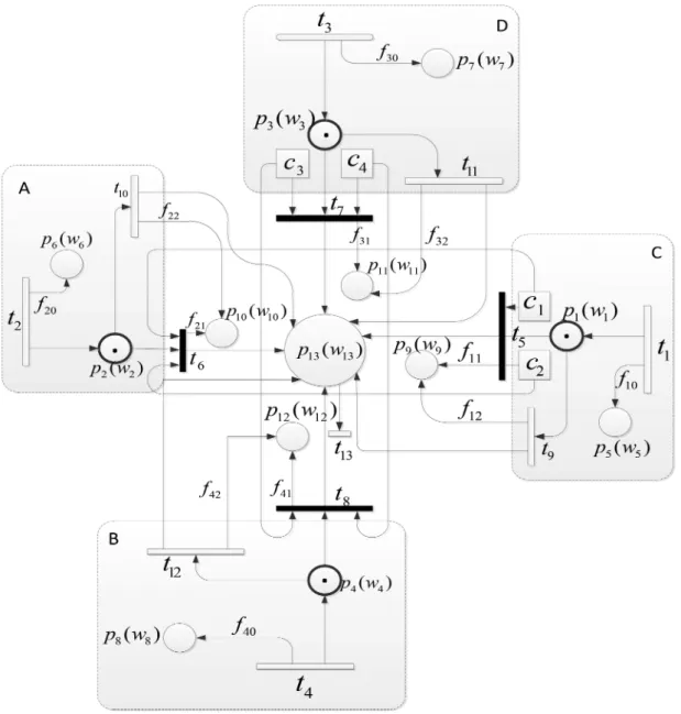
(13) In the end Fig. 2 illustrates the T-CPS model based on CSTPNs as follows.

4 CSTPN theory use on TICCS

4.1 Traffic test bed

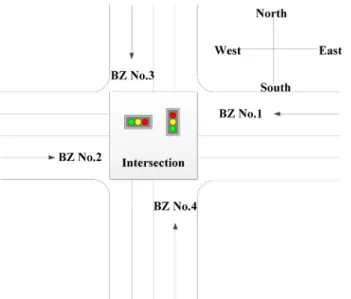
At the traffic intersection, all vehicles were assumed to pass the buffer zone (BZ) area before entering the intersection. The BZ is normally a right lane area in front of the traffic intersection about 30 m [9, 28]. The traffic intersection in Fig. 3 has four BZs, and they are BZ No.1, BZ No.2, BZ No.3 and BZ No.4. Also, traffic flows come from four different directions, and they are from South

Fig. 1 Architecture of CSTPNs

to North (SN), from North to South (NS), from East to West (EW) and from West to East (WE).

With the support of CSTPNs, T-CPS can offer the solution to the state space explosion problem by describing spatiotemporal characteristics of transportation flows in different colours and traffic light controls in TICCS. The whole traffic flow can be viewed as two parts: part 1 consists of NS and WE traffic flows and part 2 consists of SN and EW traffic flows.

4.2 TICCS formula

For the purpose of TICCS optimisation and avoid the state space

explosion, the coloured function

C(picoloured, ticoloured) = Injk, Oujk, Rojk| j = 1, 2, 3, 4; k ∈ Z is

developed to describe the attributes and states of traffic physical entities. Fig. 4 gives the phase design of traffic light control at the

traffic intersection, and TICCS using T-CPS-based CSTPNs is defined as a seven-tuple function

f_TICCS=< P, T, C(picoloured, ticoloured), Pre, Pos, Con, Wk(pi, tj) >

(14) where P = p1, p2, …, p13 is the place set of traffic physical

entities at intersection; T = t1, t2, …, t13 is the transition set of traffic cyber states at intersection; C < S >= C(picoloured, ticoloured)

associates with each element in P ∪ T that is a non-empty ordered

colour set in the possible colour set, and; _C(picoloured_{, ti}coloured₎ maps each place p_i∈ P and each transition t_i∈ T to the possible token

colour set _C(picoloured_{, ti}coloured_{) =}

In_jk, Oujk, Rojk| j = 1, 2, 3, 4; k ∈ Z ⊆ C(picoloured, ticoloured);

C < S >= C(Pcoloured_{, T}coloured_{) = {(Per}coloured_{, Con}coloured_{, Act}coloured_{, Eve}coloured_),

T = {T1, T2, …}, P = {P1, P2, …},

(Hucoloured_{, Ve}coloured_{, Ro}coloured_{, En}coloured_)},

E ⊆ P × T ∪ T × P = {True, False}, W ⊆ P × T ∪ T × P = {0, 1}, SR ⊆ P × P,

D: real number of P; R: resource of media P;

S_tat0 _{: initial states of traffic physical object;} where

C(Pcoloured_{, T}coloured_{)records the types of traffic physical objects and cyber elements;}

T is a transitions set of traffic physical object states; P is a set of places about traffic physical objects; E is an arc set that connects P with T;

W is a weight set for E;

SR presents the spatial relationship among traffic physical object places; D presents the durations among places;

R presents the media places; and S_tat0 _{is an initial state}

M_j:{status} × P = {0, 1},

Ca_j:{status} × P = { < Hucoloured_{, Ve}coloured_{, Ro}coloured_{, En}coloured_{> , null},}

Ad_j:{status} × P = { < x, y, z > , null},

Pt_j:{status} × P = { < the real number of P > , null}, Ms_j:{status} × T = {True, False}

Pt_j(P) =

min (Ptj− 1(P) + τ, D(P)), for ¬(E(Ti, P) ∧ Wj(Ti, P) = 1) ∧ Mj(P) = 1 0, for E(Ti, P) ∧ Wj(Ti, P) = 1

null, otherwise

(11)

Adj(P) =

AF(Adj− 1(Pk), Caj− 1(Pk), Caj− 1(P), SR(Pk, P)), for E(Pk, Ti) ∧ E(Ti, P) ∧

Mj(P) = 1 ∧ Mj(Pk) = 1 SF(P, Ptj(P)), for Mj(P) = 1 ∧ ¬(∃PkSR(Pk, P))

Ad_{j− 1}(Pk), for E(Pk, Ti) ∧ E(Ti, P)

null, for Mj(P) = 0

Ad_{j− 1}(P), otherwise

Con = c1, c2, c3, c4 is the control place set, and In_jk, Oujkand Rojk present the moments of the vehicle arrive,

departure and turn right at the time No._k in BZ No._j, respectively;

Pre, Pos are the pre-incidence and post-incidence matrices, respectively; and Wk (pi, tj) is a weight function as a criteria

condition concerning the number of coloured tokens in the place pi

at time t_j. For W_k (p_i, t_j) = m with _{m ∈ C(pi}coloured_{, ti}coloured₎ between p_i∈ P and t_i∈ T, if there are m tokens in p_i, the criteria condition prevents the t_j firing.

4.3 TICCS design model

The above innovative theory describes the hybrid characteristics of TICCS using the places and transitions. The theory application is useful for solving the problem concerning the state space explosion using a coloured set. Fig. 5 gives TICCS using T-CPS-based CSTPNs. There are four continuous PNs and one discrete sub-PN in this TICCS. The continuous sub-sub-PN presents the spatial flow model and the discrete sub-PN presents the discrete traffic lights scheduling model. The TICCS components are the signalised intersections, links, vehicles and traffic lights. In TICCS, the places represent the linking cells of BZ No.i or crossing sections at intersection, the tokens are running vehicles and the token colours represent the paths that vehicles are following and each cell can accommodate the time of vehicles. CSTPNs can model the signal

timing plans of traffic lights for traffic control operations at intersections.

In this above TICCS, the places p1, p2, p3, p4and p13 present BZ No.1, BZ No.2, BZ No.3, BZ No.4 and the described intersection, respectively. The places of coloured p₅, p6, …, p12 present the time

of vehicles that are entering or leaving BZ (see Table 1). The coloured transitions t1, t2, …, t13 in Table 2 describe the coloured tokens and these coloured tokens are listed in Table 3. When a transition fires, the colour of a token produced or consumed is indicated using different arc inscriptions f_ij. Some arc inscriptions are shown besides the arcs, but such arc inscriptions are ignored if their values have no influence on the model.

Table 4 gives the weight function description. Table 5 gives the physical meanings of the inputting control places. All meanings and values are the further explanation of the parameters in (14) based on the typical intersection with the normal phase design and the TICCS design model (see Figs. 3–5).

4.4 Waiting time theory

In terms of the real-time intersection control using the proposed

TICCS, the total waiting time of all vehicles in BZ No.k is recorded

as TTk

Fig. 2 T-CPS model based on CSTPNs

Fig. 3 Traffic flow at intersection Fig. 4 Intersection phase design

Fig. 5 TICCS using T-CPS-based CSTPNs

Table 1 Meanings of places

Places Meanings Places Meanings

p₁ BZ No.1 p₂ BZ No.2

p3 BZ No.3 p4 BZ No.4

p₅ the moment of vehicles enter p₁ records cache p₆ the moment of vehicles enter p₃ records cache

p7 the moment of vehicles enter p4 records cache p8 the moment of vehicles enter p5 records cache

p₉ the moment of vehicles leave p₁ records cache p₁₀ the moment of vehicles leave p₂ records cache

p11 the moment of vehicles leave p3 records cache p12 the moment of vehicles leave p4 records cache

p₁₃ the described intersection

Table 2 Meanings of transitions

Transitions Meanings Transitions Meanings

t1 vehicles enter BZ No.1 t2 vehicles enter BZ No.2

t₃ vehicles enter BZ No.3 t₄ vehicles enter BZ No.4

t5 vehicles leave BZ No.1 t6 vehicles leave BZ No.2

t₇ vehicles leave BZ No.3 t₈ vehicles leave BZ No.4

t₉ vehicles leave _BZ No.1 and turn right t₁₀ vehicles leave _BZ No.2 and turn right

t11 vehicles leave BZ No.3 and turn right t12 vehicles leave BZ No.4 and turn right

TT1=

∑

∑

∑

∑

∑

∑

∑

∑

where M_i is an arbitrary current marking; T_current is the current time; and C₅, C6, …, C12 presents the coloured tokens set in the

places of p₅, p6, …, p12.

The total vehicular waiting time (TT_SN) in SN, the total vehicular waiting time (TT_EW) in EW, the total vehicular waiting time (TT_SN) in SN and the total vehicular waiting time (TT_EW) in EW are calculated by using (16)

TT_SN= TT3+ TT4 TT_EW= TT1+ TT2 TT_SN= _MTTSN 3+ M4 TTEW= _MTTEW 1+ M2 (16)

The difference of the total vehicular waiting time _ΔTTEWNS

between EW and NS, the difference of the total vehicular waiting

time ΔTT_NSEW between NS and EW, the difference of the average

vehicular waiting time ΔTT_EWNS between EW and NS and the

difference of the average vehicular waiting time ΔTT_NSEW between

NS and EW are calculated by using (17)

ΔTT_EWNS= TT_EW− TT_NS ΔTTEWNS= TTEW− TTNS ΔTTNSEW= TTNS− TTEW ΔTT_NSEW= TT_NS− TT_EW

(17)

On the other hand, the mean error (ME) over a period TT is estimated in (18) [29] MEi= 1_TT

∫

where ϕ_isimulated_{(τ) presents the simulation flows; and; ϕ} i measured_(τ)

presents the corresponding measured flows.

To obtain the maximum vehicles passing the intersection per unit time and get the minimum average waiting time in the new TICCS, it is necessary to select the lower limit X, Y of the average vehicular waiting time in different directions. Júlvez and Boel [9] described the detail information related to the selection of the

lower limit X, Y. The real-time intersection control process

involves the following five steps:

i. If the light of the direction SN is green and the direction EW

shows the red light, then TICCS would execute the next step, or else TICCS would execute the third step.

ii. If ΔTT_EWNS≥ X or ΔTT_EWNS≥ Y, the green light of SN is switched into an yellow colour, and wait until there is no vehicle in the direction SN, then the red light of EW would be switched into a green colour.

iii. If the light of the direction EW is green, the light of the direction SN is red, then it would execute the next step.

Table 3 Meanings of coloured tokens

Tokens Meanings Tokens Meanings

C(p1coloured, t1coloured) vehicles enter p1 C(p2coloured, t2coloured) vehicles enter p2

C(p3coloured, t3coloured) vehicles enter p3 C(p4coloured, t4coloured) vehicles enter p4

C(p5coloured, t5coloured) vehicles leave p1 C(p6coloured, t6coloured) vehicles leave p2

C(p7coloured, t7coloured) vehicles leave p3 C(p8coloured, t8coloured) vehicles leave p4

C(p9coloured, t9coloured) vehicles leave p1 and turn right C(p10coloured, t10coloured) vehicles leave p2 and turn right

C(p11coloured, t11coloured) vehicles leave p3 and turn right C(p12coloured, t12coloured) vehicles leave p4 and turn right

C(p13coloured, t13coloured) vehicle leave the intersection Table 4 Meanings of weight functions

Weight function Meanings

W₁(pi, tj) = 4, (k = 1, j = 1, 2, 3, 4) C(pcolouredj , tcolouredj ) = (In11, In21, In31, In41)

W₂(pi, tj) = 4(k = 2, j = 1, 2, 3, 4) C(pcolouredj , tcolouredj ) = (Ou12, Ou22, Ou32, Ou42)

W3(pi, tj) = 4(k = 3, j = 1, 2, 3, 4) C(pcolouredj , tcolouredj ) = (Ro13, Ro23, Ro33, Ro43)

W₄(pi, tj) = 1(k = 4) C(p₁₃coloured, t₁₃coloured)

Table 5 Physical meanings of inputting control places

Control places (SN–NS) Red light Yellow light Green light Control places (WE–EW) Red light Yellow light Green light

c₁ 0 1 1 c₁ ∗ ∗ ∗

c2 0 0 1 c2 ∗ ∗ ∗

c₃ ∗ ∗ ∗ c₃ 0 1 1

c₄ ∗ ∗ ∗ c₄ 0 0 1

‘∗’ presents c₁, c2, c3, c4 can select 0 or 1.

iv. If ΔTTNSEW≥ X or ΔTTNSEW≥ Y, the green light of EW is

switched to an yellow colour and then it would wait until there is no vehicle in the direction EW, then the red light of SN would be switched into a green colour.

v. If the vehicular trajectory in BZ No.3 depends on the vehicular trajectory in BZ No.1, then the vehicles in BZ No.3 cannot

enter any of the BZs reserved by the vehicles in BZ No.1.

The above process of five steps makes two rules: (a) when

ΔTT_EWNS or ΔTT_NSEW reaches the lower limit X and executes a traffic light switch, it could extend the delay of heavy traffic flow

and (b) when ΔTT_EWNS or ΔTT_NSEW reaches the lower limit Y and

executes a traffic light switch, it could guarantee that the average value of the total vehicular waiting time is not so long to make sure the vehicles have the same opportunity to pass a traffic intersection in every direction. The above five steps can avoid the deadlock [30]. The real-time intersection control process using the proposed TICCS can dynamically show the spatiotemporal hybrid characteristics and accurately make the scheduling schemes.

5 Experimental simulation study

Given that the traffic simulation scenario has two-lane roads with one lane in each direction (see Fig. 3), the transit time is the time taken from the marked start-point in the front of the intersection to the marked end-point behind the intersection. The transit time is related to the intersection phase design in Fig. 4. The transit time of the vehicles created by the simulation model maybe different from the transit time of the vehicles with a constant velocity and non-stop at the intersection. This transit time difference is viewed as a transit delay due to the intersection traffic interference. The average transit delay of all vehicles can be calculated for the simulation analysis.

Also, there are some additional assumption conditions in the traffic simulation study analysis. Traffic simulation has a Poisson random distribution at the four-way perfect-cross intersection. Traffic flow is homogeneous, that is, there is the equal amount of traffic volume in every direction with an equal amount of vehicular turning ratios. Moreover, the average traffic flow rate of each intersection direction has a range between 0.1 vehicles per second and 1 vehicle per second. The whole traffic simulation is implemented for 100 times, the simulation data each time involve 1000 vehicles. After the last vehicle leaves away from the intersection, the simulation would be terminated. The traffic parameters ϕ_isimulated_{(τ) and ϕ}

i

measured_{(τ) present the simulated traffic}

flows and the measured traffic flows at the end of each road stretch, respectively. Febbraro and Sacco [8] used the two parameters for the ME calculation.

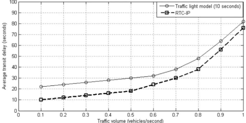
In contrast to the traffic light model with 10 s green light time [31], the average transit delay of real-time control intersection protocol (RTC-IP) is much lower, as shown in Fig. 6. The RTC-IP has totally 39.24% improvement over the traffic light model (10 s). When traffic simulation volumes were changed at that intersection and traffic density from the SN direction was higher than the EW direction, the RTC-IP model gave much better data results than the traffic light model, as shown in Fig. 7.

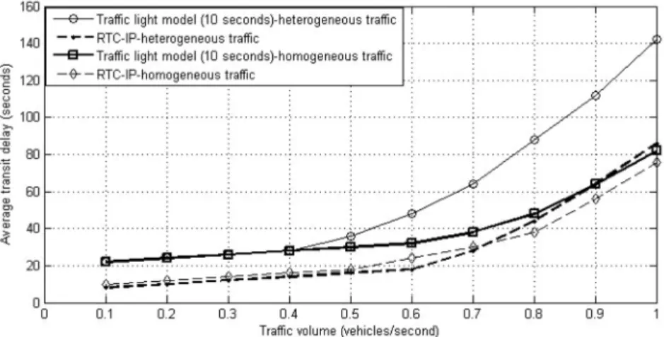
Fig. 8 shows the comparison between the heterogeneous traffic (different traffic volumes from the intersection directions) and the homogeneous traffic via the use of RTC-IP and the traffic light model (10 s). A higher traffic density would cause a higher delay, that is, the average transit delay would be higher. The difference of the average transit delay between the heterogeneous traffic and the homogeneous traffic was inconsistent for RTC-IP and the traffic light model. In terms of the traffic light model, a higher traffic volume caused a higher average transit delay and the heterogeneous traffic had a more significant increase than the

Fig. 6 Average transit delay of traffic light model and RTC-IP

homogeneous traffic. However, in RTC-IP a higher traffic volume also caused a higher average transit delay and the heterogeneous traffic had a similar increase to the homogeneous traffic. It implies that the RTC-IP can achieve more vehicles to pass the intersection over the same time period with a less waiting time.

To evaluate the model accuracy, Table 6 gives the ME results

(ME_i) of the RTC-IP and the traffic light model. It shows that the

TICCS using T-CPS-based CSTPNs can offer a better result in data accuracy, the ME of the RTC-IP was less than the traffic light model in BZ Nos. 1, 2 and 4, except BZ No. 3.

6 Theory implementation

T-CPS-based CSTPNs is a new theory in the information application for the improvement of traffic control system performance. To realise a better secure and efficient dynamic traffic control operation, the performance of T-CPS-based CSTPNs theory is the integration of traffic physical, information and behaviour processes on the configuration and deployment of the traffic control CPS system (see Fig. 9). This elaborate and coordinate paradigm involves three levels, i.e. the integration of information and transportation processes using T-CPS-based CSTPNs theory, traffic data detection and collection, the technical solution and support of modern computing, communication and control technologies.

Also, the traffic environment is a real dynamic physical world and the cyberspace is a virtual world. Fig. 10 gives the interaction between the cyberspace and the physical world for traffic control CPS. The data detection, information communication and auto computation, related to T-CPS-based CSTPNs theory, are the core of this interaction. In fact, the interaction between the cyberspace

Fig. 8 Average transit delays of heterogeneous and homogeneous traffic data

Table 6 MEs comparison (10 s)

BZs RTC-IP Traffic light model (10 s)

BZ No 1 _{5.6 × 10}−5 _{7.1 × 10}−5

BZ No 2 _{−8.7 × 10}−3 _{−9.3 × 10}−3

BZ No 3 _{1.2 × 10}−2 _{0.96 × 10}−2

BZ No 4 _{1.6 × 10}−2 _{1.8 × 10}−2

Fig. 9 Integration of traffic physical, information and behaviour processes [32]

and the physical world is a mapping concerning traffic control comprehensive information of the traffic PS, process and behaviour.

7 Concluding remarks

On the basis of the CTPN theory, this paper develops the CSTPN theory for the description of the discrete-continuous hybrid T-CPS, and then applies the new CSTPN theory for the development of TICCS. These research theories and methods can not only reveal the inherent spatiotemporal characteristics of T-CPS, but also solve the state space explosion problem using coloured tokens sets. Using the modelling and simulation analyses, this paper demonstrates that the proposed approaches can effectively handle dynamic traffic interactions from all directions of traffic intersections to reduce the average transit delays and the MEs. In addition, these theories and methods created have a good validity and practicality for the development of T-CPS.

Further research may develop verification platforms or methods for the development of T-CPSs with different road or intersection geometrical features and more complicate traffic simulation situations. Also, it would be useful for dynamic information optimisation and traffic delay analysis via the integration of CSTPNs, advanced traffic event data collection techniques [33], advanced traffic data models [34] and spatiotemporal transportation databases [35].

8 Acknowledgments

The authors gratefully acknowledge the research funding support from the National Natural Science Foundation of China (NSFC) (Grant No. 61573075), the core projects of Chongqing City ‘151’ science and technology (Grant No. cstc2013jcsf-zdzxqqX0003), National Key R&D Program (Grant No. 2016YFB0100904), Scientific and Technological Research Program of Chongqing Municipal Education Commission (Grant No. KJ1503301) and the Fundamental Research Funds of China Central Universities (Grant No. 10611214CDJZR178801).

9 References

[1] Yue, H., Yang, R.J.: ‘Development of intelligent transportation systems and plan of integrated information system’, J. Wuhan Univ. Technol., 2005, 109, (1), pp. 57–70

[2] Sun, D.H., Li, Y.H., Liu, W.N., et al.: ‘Research summary on transportation cyber physical systems and the challenging technologies’, Zhongguo Gonglu Xuebao (China J. Highway Transp.), 2013, 26, (1), pp. 144–154

[3] Yue, H., Revesz, P.Z.: ‘TVICS: an efficient traffic video information converting system’, 19th Int. Symp. on Temporal Representation and Reasoning (TIME), (Prentice Hall inc, NJ, 2012), pp. 141–148

[4] Peterson, J.L.: ‘Petri net theory and the modeling of systems’, 1981 [5] Murata, T.: ‘Petri nets: properties, analysis and applications’, Proc. IEEE,

1989, 77, (4), pp. 541–580

[6] Girault, C., Valk, R.: ‘Petri nets for systems engineering: a guide to modeling, verification, and applications’ (Springer Science and Business Media, Berlin, 2003)

[7] Huang, H., Kirchner, H.: ‘Policy composition based on Petri nets’. 33rd Annual IEEE Int. Computer Software and Applications Conf., COMPSAC'09, 2009

[8] Febbraro, A.D., Sacco, N.: ‘On modelling urban transportation networks via hybrid Petri nets’, Control Eng. Pract., 2004, 12, (10), pp. 1225–1239 [9] Júlvez, J., Boel, R.K.: ‘A continuous Petri net approach for model predictive

control of traffic systems’, IEEE Trans. Syst. Man Cybern. A, Syst. Hum., 2010, 40, (4), pp. 686–697

[10] Ng, K.M., Reaz, M.B.I., Ali, M.A.M.: ‘A review on the applications of Petri nets in modeling, analysis, and control of urban traffic’, IEEE Trans. Intell. Transp. Syst., 2013, 14, (2), pp. 858–870

[11] Febbraro, A.D., Giglio, D., Sacco, N.: ‘On applying Petri nets to determine optimal offsets for coordinated traffic light timings’. Proc. The IEEE Int. Conf. on Intelligent Transportation Systems, 2002, 2002

[12] Haghighi, I., Jones, A., Kong, Z., , et al.: ‘SpaTeL: a novel spatial–temporal logic and its applications to networked systems’. Proc. of the 18th Int. Conf. on Hybrid Systems, Computation and Control, 2015, pp. 189–198

[13] Wu, H., Chen, Y., Zhang, M.: ‘On denotational semantics of spatial-temporal consistency language – SteC’. 2013 Int. Symp. on Theoretical Aspects of Software Engineering (TASE), 2013

[14] Mu, Y., Wu, J., Jenkins, N., et al.: ‘A spatial–temporal model for grid impact analysis of plug-in electric vehicles’, Appl. Energy, 2014, 114, pp. 456–465 [15] Chi, M., Yubin, H., Yongyong, Z., et al.: ‘Spatial–temporal indexing research

based on road network: improved-MON-tree’, Int. J. Hybrid Inf. Technol., 2014, 7, (4), pp. 407–416

[16] Kloog, I., Chudnovsky, A.A., Just, A.C., et al.: ‘A new hybrid spatio-temporal model for estimating daily multi-year PM 2.5 concentrations across northeastern USA using high resolution aerosol optical depth data’, Atmos. Environ., 2014, 95, pp. 581–590

[17] Shao, Z., Liu, J.: ‘Spatio-temporal hybrid automata for cyber-physical systems’, In: Liu, Z., Woodcock, J., Zhu, H. (eds): ‘International colloquium on theoretical aspects of computing (ICTAC)’, (Springer, Berlin Heidelberg), 2013, pp. 337–354

[18] Thong, W.J., Ameedeen, M.A.: ‘A survey of Petri net tools’, in Sulaiman, H.A., Othman, M.A., Othman, M.F.I, Pee, N.C., Rahim, Y.A., Pee, N.C. (EDs.): ‘Advanced Computer and Communication Engineering Technology’ (Springer International Publishing, 2015), pp. 537–551

[19] Zhang, G., Zhang, M., Yan, R., et al.: ‘Modeling and analysis for CPS physical entities based on spatio-temporal Petri net’, J. Comput., 2014, 9, (2), pp. 499–505

[20] Aized, T.: ‘Modelling and performance maximization of an integrated automated guided vehicle system using coloured Petri net and response surface methods’, Computers & Industrial Engineering, 2009, 57, (3), pp. 822–831

[21] Huang, Y.S., Chung, T.H.: ‘Modelling and analysis of air traffic control systems using hierarchical timed coloured Petri nets’, Trans. Inst. Meas. Control, 2011, 33, (1), pp. 30–49

[22] List, G.F., Cetin, M.: ‘Modeling traffic signal control using Petri nets’, IEEE Trans. Intell. Transp. Syst., 2004, 5, (3), pp. 177–187

[23] Cheng, Y.H., Yang, L.A.: ‘A fuzzy Petri nets approach for railway traffic control in case of abnormality: evidence from Taiwan railway system’, Expert Syst. Appl., 2009, 36, (4), pp. 8040–8048

[24] Silva, M., Recalde, L.: ‘On fluidification of Petri nets: from discrete to hybrid and continuous models’, Annu. Rev. Control, 2004, 28, (2), pp. 253–266 [25] Dotoli, M., Fanti, M.P., Iacobellis, G.: ‘An urban traffic network model by

first order hybrid Petri nets’. IEEE Int. Conf. on Systems, Man and Cybernetics, SMC 2008, 2008, pp. 1929–1934

[26] J, űlvez, J.J., Boel, R.K.: ‘A continuous Petri net approach for model predictive control of traffic systems’, IEEE Trans. Syst. Hum. Syst. Man Cybern. A, 2010, 40, (4), pp. 686–697

[27] Dotoli, M., Fanti, M.P.: ‘An urban traffic network model via coloured timed Petri nets’, Control Eng. Pract., 2006, 14, (10), pp. 1213–1229

[28] Ma, N.: ‘Influence factors of coordination control system in signalized intersections’, Harbin Gongye Daxue Xuebao (J. Harbin Inst. Technol.), 2011, 43, (6), pp. 112–117

[29] Di Febbraro, A., Sacco, N.: ‘On modelling urban transportation networks via hybrid Petri nets’, Control Eng. Pract., 2004, 12, (10), pp. 1225–1239 [30] Perronnet, F., Abbas-Turki, A., El Moudni, A.: ‘Vehicle routing through

deadlock-free policy for cooperative traffic control in a network of intersections: reservation and congestion’. 2014 IEEE 17th Int. Conf. on. Intelligent Transportation Systems (ITSC), 2014, pp. 2233–2238

[31] Azimi, R., Bhatia, G., Rajkumar, R., et al.: ‘Intersection management using vehicular networks’, SAE Technical Paper, 2012

[32] Jianjun, S., Xu, W., Jizhen, G., et al.: ‘The analysis of traffic control cyber-physical systems’, Procedia, Soc. Behav. Sci., 2013, 96, pp. 2487–2496 [33] Liu, C., Sharma, A., Smaglik, E., et al.: ‘TraSER: a traffic signal event-based

recorder’, Softwarex, 2016, 5, pp. 156–162

[34] Yue, H., Jones, E.G., Revesz, P.: ‘Local polynomial regression models for average traffic speed estimation and forecasting in linear constraint databases’. 2010 17th Int. Symp. on Temporal Representation and Reasoning (TIME), 2010, pp. 154–161

[35] Yue, H., Rilett, L.R., Revesz, P.Z.: ‘Spatio-temporal traffic video data archiving and retrieval system’, GeoInformatica, 2016, 20, (1), pp. 59–94