University of Wisconsin Milwaukee
UWM Digital Commons
Theses and DissertationsAugust 2018
Developing a Probabilistic Heavy-Rainfall
Guidance Forecast Model for Great Lakes Cities
Cory Kevin Rothstein
University of Wisconsin-Milwaukee
Follow this and additional works at:https://dc.uwm.edu/etd
Part of theAtmospheric Sciences Commons
This Thesis is brought to you for free and open access by UWM Digital Commons. It has been accepted for inclusion in Theses and Dissertations by an authorized administrator of UWM Digital Commons. For more information, please [email protected].
Recommended Citation
Rothstein, Cory Kevin, "Developing a Probabilistic Heavy-Rainfall Guidance Forecast Model for Great Lakes Cities" (2018).Theses and Dissertations. 1911.
DEVELOPING A PROBABILISTIC HEAVY-RAINFALL GUIDANCE FORECAST MODEL FOR GREAT LAKES CITIES
by Cory Rothstein
A Thesis Submitted in Partial Fulfillment of the Requirements for the Degree of
Master of Science in Atmospheric Science
at
The University of Wisconsin-Milwaukee August 2018
ABSTRACT
DEVELOPING A PROBABILISTIC HEAVY-RAINFALL GUIDANCE FORECAST MODEL FOR GREAT LAKES CITIES
by Cory Rothstein
The University of Wisconsin-Milwaukee, 2018 Under the Supervision of Professor Paul Roebber
A method for predicting the probability of exceeding specific warm-season (April-October) 0-24 hour precipitation thresholds is developed based upon daily maximums of
meteorological parameters. North American Regional Reanalysis and Daily Unified Precipitation data from 2002-2017 were used to gather meteorological data for the Milwaukee and Chicago County Warning Areas. Individual artificial neural networks and multiple logistic regressions were conducted for daily rainfall thresholds above 0.5'', 1'', 1.5'' and 2'' to determine the probability of threshold exceedances for each County Warning Area. The most important
parameters were 1000-500 hPa specific humidity, vertical velocities at various levels, high cloud cover, precipitable water percentile relative to climatology, and surface convergence. Critical Success Indices were universally higher than the average 2017 warm-season WPC threat scores across all thresholds, showing potential promise in operational forecasting use. Sensitivity analyses were conducted to determine degradation of model results when using NWP model forecasts, with mixed results between the two cases studied. Future work includes using additional years of reanalysis and rainfall data to increase heavy-rainfall case counts and boost model skill, as well as to include additional case studies to further analyze model degradation when using NWP model forecasts.
TABLE OF CONTENTS
I. INTRODUCTION...1
II. METHODOLOGY...6
a. Data and Parameter Selection...6
b. Model Construction...8
III. RESULTS AND VERIFICATION...12
a. MLR and MLP ANN model results......12
b. Sensitivity analysis...15
c. Model degradation case studies...18
IV. CONCLUSIONS AND FUTURE WORK...23
V. REFERENCES...51
VI. APPENDIX...53
a. MLR Equations for the Milwaukee CWA...53
b. MLR Equations for the Chicago CWA....54
c. MLP ANN Equations for the Milwaukee CWA......55
d. MLP ANN Equations for the Chicago CWA.......59
e. Multiple (least squares) linear regression equation for the Milwaukee and Chicago CWAs MLR and ANN exceedance probability thresholds.....63
LIST OF FIGURES
Figure 1. A map showing the Milwaukee (MKX) and Chicago (LOT) National Weather Service (NWS) county warning areas (CWAs) outlined in red (NWS 2018b)...32
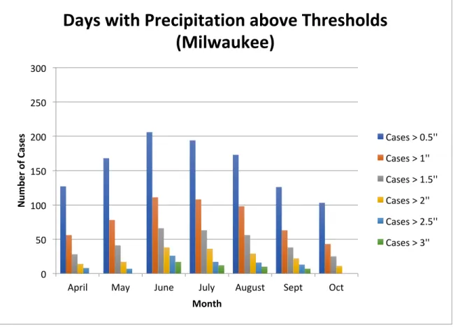
Figure 2. A histogram showing the number of days with precipitation thresholds above 0.5 in. (blue), 1.0 in. (orange), 1.5 in. (gray), 2.0 in. (yellow), 2.5 in. (light blue), and 3.0 in. (green) stratified by month for the Milwaukee CWA...33
Figure 3. A histogram showing the number of days with precipitation thresholds above 0.5 in. (blue), 1.0 in. (orange), 1.5 in. (gray), 2.0 in. (yellow), 2.5 in. (light blue), and 3.0 in. (green) stratified by month for the Chicago CWA...34
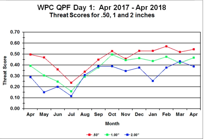
Figure 4. WPC Day 1 Quantitative Precipitation Forecast (QPF) threat scores for 0.50 in., 1 in. and 2 in. by month for April 2017 to April 2018 (Weather Prediction Center 2018)...35
Figure 5. The regional domain used to average the NARR 32-km data for every 3-hour interval between April-October of 2002-2017...36
Figure 6. The sub-domains used to average the NARR 32-km data for every 3-hour interval between April-October of 2002-2017. The red box shows the domain used for the Milwaukee CWA, while the purple box shows the domain used for the Chicago CWA...37
Figure 7. Correlation values for the maximum daily precipitation (maxp) and variables being input into the MLR and MLP ANNs for the Milwaukee CWA. Correlations range from -1 to 1, with negative values denoting negative correlations and positive values denoting positive
correlations...38
Figure 8. Correlation values for the maximum daily precipitation (maxp) and variables being input into the MLR and MLP ANNs for the Chicago CWA. Correlations range from -1 to 1, with negative values denoting negative correlations and positive values denoting positive
correlations...39
Figure 9. Schematic of a MLP ANN obtained from Roebber et al. (2003), including the input layer, hidden layer and output layers. For this study, the input layer is the meteorological variables being put into the model, the hidden layer involves the range of 3-6 nodes that were used for weighting, and the output layer is the probabilities of surpassing the 12.7 mm (0.5 in.), 25.4 mm (1.0 in.), 38.1 mm (1.5 in.), and 50.8 mm (2.0 in.) daily rainfall thresholds...40
Figure 10. Performance diagram (Roebber 2009) for the Milwaukee CWA. Red shapes indicate MLP ANNs and black shapes indicate MLR models. Circles represent the P ≥ 25.4 mm (1 in.) threshold, squares represent the P ≥ 38.1 mm (1.5 in.) threshold, and stars represent the P ≥ 50.8 mm (2 in.) threshold. Bias is shown in the dashed line, CSI is shown in the solid curved lines, success ratio (1-FAR) is shown on the x-axis and POD is shown on the y-axis...41
Figure 11. Performance diagram (Roebber 2009) for the Chicago CWA. Red shapes indicate MLP ANNs and black shapes indicate MLR models. Circles represent the P ≥ 25.4 mm (1 in.) threshold, squares represent the P ≥ 38.1 mm (1.5 in.) threshold, and stars represent the P ≥ 50.8 mm (2 in.) threshold. Bias is shown in the dashed line, CSI is shown in the solid curved lines, success ratio (1-FAR) is shown on the x-axis and POD is shown on the y-axis...42
Figure 12. 24-hour rainfall accumulations ending 1200 UTC 8 September 2016 for the upper Midwest, obtained from the Advanced Hydrologic Precipitation Service Precipitation Analysis (NWS 2018a). Precipitation amounts (in inches) are denoted by the colorbar on the lefthand side of the image...43
Figure 13. (a)-(d) Sensitivity analysis results for the Milwaukee CWA for: (a) Daily maximum 1000-500 hPa mean specific humidity (MAXSHUM; kg/kg), (b) daily minimum 300 hPa vertical motion (MINOMEGA300; Pa/s), (c) daily maximum high cloud fraction (MAXHCDC; %), and (d) daily maximum surface convergence (MINDMAX; *10^(-5)/s). The lines indicate
probabilities of exceedance for the P ≥ 12.7 mm (blue), P ≥ 25.4 mm (red), P ≥ 38.1 mm (green), and P ≥ 50.8 mm (purple) MLP ANN model thresholds...44
Figure 14. (a)-(d) Sensitivity analysis results for the Milwaukee CWA for: (a) Daily maximum 1000-500 hPa mean specific humidity (MAXSHUM; kg/kg), (b) daily minimum 500 hPa vertical motion (MINOMEGA500; Pa/s), (c) daily minimum 850 hPa vertical motion (MINOMEGA850; Pa/s), and (d) daily maximum high cloud fraction (MAXHCDC; %). The lines indicate
probabilities of exceedance for the P ≥ 12.7 mm (blue), P ≥ 25.4 mm (red), P ≥ 38.1 mm (green), and P ≥ 50.8 mm (purple) MLP ANN model thresholds...45
Figure 15. (a)-(d) Probabilities of threshold exceedance (%) for the MLR vs. ANN models in the Milwaukee CWA for the (a) P ≥ 12.7 mm, (b) P ≥ 25.4 mm, (c) P ≥ 38.1 mm, and (d) P ≥ 50.8 mm thresholds. Red circles denote cases where the daily observed maximum precipitation was above the threshold level, while blue circles denote daily observed maximum precipitation that was below the threshold level...46
Figure 16. (a)-(d) Probabilities of threshold exceedance (%) for the MLR vs. ANN models in the Chicago CWA for the (a) P ≥ 12.7 mm, (b) P ≥ 25.4 mm, (c) P ≥ 38.1 mm, and (d) P ≥ 50.8 mm thresholds. Red circles denote cases where the daily observed maximum precipitation was above the threshold level, while blue circles denote daily observed maximum precipitation that was below the threshold level...47
Figure 17. 24-hour rainfall accumulations ending 1200 UTC 9 April 2013 for the upper Midwest, obtained from the Advanced Hydrologic Precipitation Service Precipitation Analysis (NWS 2018a). Precipitation amounts (in inches) are denoted by the colorbar on the lefthand side of the image...48
Figure 18. (a)-(d) Base reflectivity taken during the period from 1200 UTC 8 April 2013 to 12 UTC 9 April 2013 at (a) 15 UTC, (b) 18 UTC, (c) 21 UTC, and (d) 12 UTC 9 April. Images were obtained from the UCAR image archive at http://www2.mmm.ucar.edu/imagearchive/
Figure 19. (a)-(d) Base reflectivity taken during the period from 1200 UTC 7 Sept. 2016 to 1200 UTC 8 Sept. 2016 at (a) 12 UTC, (b) 18 UTC, (c) 21 UTC, and (d) 12 UTC 8 Sept. Images were obtained from the UCAR image archive at http://www2.mmm.ucar.edu/imagearchive/
LIST OF TABLES
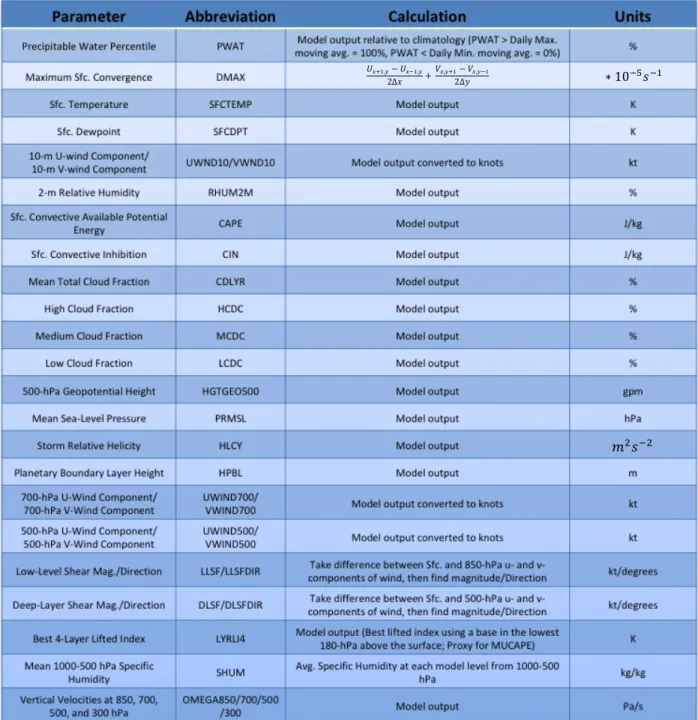
Table 1. A list of the initial 31 meteorological variables included in this study, with their
abbreviations, calculations and units displayed in the table...26
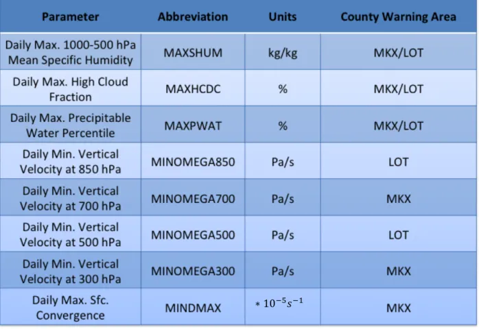
Table 2. A list of the final variable list that was used for the MLR and MLP ANN models, with their abbreviations, units, and which county warning area (CWA) they were used for. MKX denotes variables used in the Milwaukee CWA models, while LOT denotes variables used in the Chicago CWA models...27
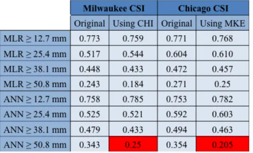
Table 3. Critical Success Index (CSI) scores for the test data in the Milwaukee and Chicago CWAs across all threshold levels for both the MLR and MLP ANN using the original predictors for each CWA, as well as using the respective predictors from the other CWA. Boxes
highlighted in red show where CSI scores dropped by more than 5% by using the other CWA’s predictors relative to the original predictors...28
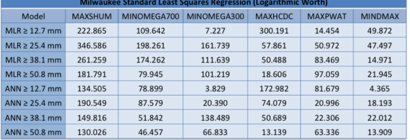
Table 4. Logarithmic worth of each variable for the standard least squares regression for all MLR and ANN probability exceedance thresholds for the Milwaukee CWA...29
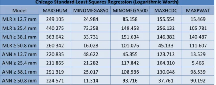
Table 5. Logarithmic worth of each variable for the standard least squares regression for all MLR and ANN probability exceedance thresholds for the Chicago CWA...30
Table 6. Probabilities of threshold exceedances for the Milwaukee and Chicago CWAs across all threshold levels for both the MLR and MLP ANN models for 8-9 April 2013 and 7-8 Sept. 2016. NARR columns denote original probabilities using values for the input variables from the NARR dataset, while probabilities in the NAM columns are using NAM data. Boxes highlighted in red show thresholds were probabilities dropped by more than 10% by using the NAM data, while boxes highlighted in green show a more than 10% increase in probabilities using the NAM data...31
ACKNOWLEDGEMENTS
I would like to thank Professor Paul Roebber for his guidance as my advisor throughout this research, as well as his constant assistance with Fortran 77 scripting. I would also like to thank Professor Clark Evans for his assistance with GrADS scripting and futher ideas for this project and Professor Jon Kahl for being on my committee. Finally, I would like to thank NOAA Sea Grant for providing grant funding for my research assistantship and this project.
I. INTRODUCTION
According to Doswell et al. (1996), flash flooding annually produces the most fatalities of convective storm related events due, in part, to the difficulty of not only predicting the occurrence of an event, but also accurately predicting the magnitude and scope of the heavy rainfall associated with such an event. Significant vulnerabilities to flooding exist in large urban areas such as the Milwaukee and Chicago communities, with flooding risks dependent on recent and current environmental conditions in conjunction with the magnitude of heavy rainfall during an event. Examples of environmental conditions may include: pre-existing and current conditions at the surface, such as soil moisture and temperature, time since the previous precipitation event, topography of the land surface, and land use. However, the focus of this research will not be on the environmental conditions associated with flooding, but rather to improve upon heavy rainfall prediction to enhance situational awareness for weather forecasters.
The impact of heavy rainfall on communities continues to be a driving factor in improving forecasting methods, due to the demand for accurate precipitation forecasts that are used in the industry, commercial, and residential sectors, especially for extreme precipitation events (i.e. those events above the 99th percentile) (Sukovich et al. 2014). The recent analysis from Sukovich et al. (2014) found that the forecasting skill for NWS forecasts from 2001-2011 was the lowest for areas in which convective precipitation was dominant, resulting in a low probabilities of detection (PODs) and high false alarm ratios (FARs) during the warm season (May 1st – October 31st), particularly in the upper Midwest. Thus, it is necessary to improve the
To understand the nature of heavy rainfall events and their causality, it is necessary to look at environmental conditions and precipitation modes that are generally associated with heavy rainfall. The storm structures and meteorological parameters associated with heavy rainfall events have been extensively researched, with general agreement on the frequency and archetypes of storm structures that are closely correlated to heavy rainfall events. Schumacher and Johnson (2005) identified 116 total cases of “extreme” rainfall events (classified as when 24-hour precipitation totals exceed a 50-yr occurrence interval in the case of their study) during the warm seasons between 1999 and 2001 in the eastern two-thirds of the United States, of which 65 percent were determined to be mesoscale convective systems (MCSs). The MCSs were further broken down into two main patterns: training line/adjoining stratiform (TL/AS) and back-building/quasi-stationary (BB) systems. TL/AS storms typically form in very moist and unstable environments on the cold side of a pre-existing quasi-stationary surface boundary, where warm, stable air flows over the frontal zone (Maddox 1979). Peters and Roebber (2014) determined that TL/AS storms can also occur along local outflow boundaries, with deep layer wind shear roughly parallel to the boundary. BB systems are generally more dependent on storm-scale processes, such as lifting provided by cold pools rather than synoptic boundaries and are also less common than TL/AS systems.
Another set of MCS storm structures were identified by Parker and Johnson (2000), in which three main linear storm modes were determined: Trailing Stratiform (TS), Leading Stratiform (LS), and Parallel Stratiform (PS). TS storms comprised roughly 60 percent of MCS archetypes during the study, while LS and PS archetypes comprised only 20 percent of MCSs, respectively (refer to their Fig. 4). The majority of these storm systems formed in areas associated with the core or terminus of a low-level jet. Analysis shows that TS storms were the
fastest moving archetype and had durations that were twice as long when compared to the LS and PS storm archetypes. The relative strength of the cold pools for the TS archetype was the largest, followed by PS, and finally LS had the weakest archetypes. It was also noted that over 50 percent of linear MCSs evolve towards a TS structure at some point during a life cycle.
Other storm structures associated with heavy rainfall production have also been extensively researched, although MCSs remain disproportionately as the predominant storm structure for heavy rainfall and flash floods (Parker and Johnson 2004). High precipitation (HP) supercells generally produce heavy rainfall, but only occur over a relatively short period of time due to their rapid motion and small areal extent (Doswell 1996). Multicellular storms also have the potential to produce heavy rainfall for a specific area, but only if the storm duration becomes elongated due to multiple convective cells repeatedly traveling over the same location. In fact, when applied generally to heavy rainfall events, Doswell (1996) determined that substantial rainfall accumulations were due to slow storm movement, prolonged heavy rainfall rates, large areal storm extent, or a combination of these factors.
On a more general note, there are multiple meteorological parameters associated with heavy rainfall accumulations regardless of storm structure. A majority of cases involved low to moderate deep-layer wind shear with substantial low-level veering and relatively weak magnitudes, precipitable water (PW) values on the order of 150 percent or more of mean climatological values, and relative humidity (RH) values in the 1000-mb to 500-mb layer of greater than 70 percent (Moore 2003; Maddox 1979; Junker 1999; Schumacher and Johnson 2015). For cases in which surface boundaries were present, such as MCSs and frontal-type storm archetypes, storms primarily formed on the cold side and parallel to a low-level boundary, in which a southerly low-level jet was present to supply moisture feeds for the storms. Also, the
center of heaviest rainfall occurred in areas of maximum equivalent potential temperature advection, along the southern gradient of the 250-mb divergence maximum, and in areas of high 850-mb warm air advection ahead of 500-mb cut-off lows (Junker 1999).
The majority of the studies mentioned above focus on specific case studies of heavy and extreme precipitation, composite analyses over multiple cases, or numerical weather prediction (NWP) models to assess the meteorological environments associated with heavy precipitation as a method to improve situational awareness to forecasters and, subsequently, quantitative
precipitation forecasts. However, this study looks to improve upon weather model guidance through the use of a multi-layer perceptron artificial neural network (MLP ANN) as a statistical post-processing tool using various meteorological variable outputs from model guidance output in order to predict the likelihood of heavy rainfall events above certain thresholds for a 0-24 hour, Day 1 forecast for the Milwaukee and Chicago National Weather Service (NWS) county warning areas (CWAs) according to the methodology described in section 2 of this study. ANNs are one class of a wide variety of methods that perform the function of mapping inputs to
outputs. Here, the inputs are the meteorological variables identified as relevant to heavy precipitation production and the output is the probability of rainfall exceeding the threshold values chosen for this study. This forecasting tool will be developed using reanalysis data from the North American Regional Reanalysis (NARR) dataset during the warm season (April-October) from 2002-2017, with specific meteorological parameters from this dataset chosen based on their significance in connection with heavy rainfall events examined in previous research. Studying which meteorological parameters are most closely correlated with heavy rainfall events and mapping them to probabilities of rainfall exceeding specific thresholds, the goal is to improve the predictability of such events for NWS forecasters, and, in turn, increase
situational awareness for both forecasters and the communities of the Milwaukee and Chicago CWAs.
The organization of this study is as follows. Section 2 describes the data methods used in producing the MLP ANN based on previous research and other statistical methods. Section 3 describes the model results and verification process, as well as a sensitivity analysis for two specific cases. Finally, section 4 summarizes the conclusions as well as any future directions for the research.
II. METHODOLOGY
a. Data and parameter selection
In order to first classify heavy rainfall thresholds for the Milwaukee (MKX) and Chicago (LOT) CWAs (Fig. 1), the initial idea was to quantify the rainfall categories based on extreme (99th percentile) events in the North Central River Forecast Center (NCRFC) region that includes
both CWAs for this study (Sukovich et al. 2014). According to that study, rainfall over 38.1 mm (1.5 in.) averaged over 32-km grids constitutes the upper 1% of the precipitation distribution. However, the NCRFC is a relatively large region including the majority of Minnesota, Iowa, Illinois, Wisconsin and Michigan, so thresholds that are more representative of the specific CWAs were deemed necessary. This led to considering the 1-year recurrence intervals for 24-hour precipitation amounts according to NOAA Atlas 14 from the Precipitation Frequency Data Server, with the base locations of Milwaukee Mitchell Airport and Chicago O’Hare Airport used to represent the recurrence interval for the Milwaukee and Chicago CWAs, respectively (HDSC 2017). 1-yr, 24-hour recurrence intervals were found to be 2.35 inches for both CWAs, with 90-percent confidence intervals of 2.13-2.61 inches for Milwaukee and 2.10-2.64 inches for
Chicago. This threshold was a good starting point, but threshold levels were further refined after conversing with utilities that have operational experience in managing storm water flow for major urban communities, such as the Milwaukee Metropolitan Sewage District (MMSD). Finally, daily-accumulated precipitation (P) thresholds were classified into 4 categories: P ≥ 12.7 mm (0.5 in.), P ≥ 25.4 mm (1.0 in.), P ≥ 38.1 mm (1.5 in.), and P ≥ 50.8 mm (2 in.).
Heavy rainfall cases were then identified from 16 years (2002-2017) of warm-season (April-October) daily 1200 UTC-1200 UTC gridded precipitation data from the Daily U.S. Unified Precipitation dataset for verification purposes (NOAA/OAR/ESRL PSD, 2018). This
analysis was created from observations of rain gauges throughout the continental United States (CONUS) and then interpolated onto a 0.25° × 0.25° grid. The grid with the maximum daily
precipitation in each CWA was then extracted. Daily precipitation data were then screened to remove any days where precipitation amounts were less than 6.37 mm (0.25 in.) to reduce bias in the forecasts since a forecast of no major rainfall amounts is trivial for heavy rainfall prediction. This resulted in 1517 total days with rainfall above 0.25 in. for the Milwaukee CWA and 1732 total days for the Chicago CWA. After the screening process, data was binned into the
precipitation thresholds defined above, with histograms showing the number of cases above each threshold by month for the Milwaukee and Chicago CWAs shown in Figures 2 and 3,
respectively. The peak amount of days with precipitation above all threshold values in both CWAs occur during the months of June through August, which coincides with the lowest
quantitative precipitation forecast (QPFs) verification scores from the Weather Prediction Center (WPC) shown in Figure 4 (Weather Prediction Center 2018). This further highlights the need for heavy rainfall forecast improvements during the warm season when the skills are the lowest.
As stated in the “Introduction” section of this paper, meteorological variables chosen for this study were obtained from the NARR 32-km dataset for the same time period as the daily rainfall data on a 3-hourly basis for each day from 1200 UTC to 1200 UTC to coincide with the rainfall accumulation period (NOAA/OAR/ESRL PSD, 2017). Table 1 shows the initial 31 variables extracted from the NARR dataset, abbreviations for this study, calculations, and units. The majority of these variables were chosen to align closely with the variables from previous research, while some of the variables were chosen based on the necessary ingredients for thunderstorm development: lift (OMEGA, DMAX), instability (CAPE, CIN, LYRLI4), shear (LLSF, DLSF and directions), and moisture (SHUM, RHUM2M, SFCDPT). All variables were
then averaged over a large domain encompassing much of the upper Midwest, shifted upstream of the CWAs to capture synoptic conditions during each 3-hourly period (Fig. 5). Variables were also averaged over sub-domains at each 3-hour period encompassing the Milwaukee and
Chicago CWAs to capture more local signals of the meteorological variables as shown in Figure 6. This use of reanalysis data—which act as a proxy for observations—in obtaining
meteorological variables to be used as predictors in statistical models for precipitation forecasts is known as the “perfect prog” method (Vislocky and Yound 1989). There are two drawbacks that limit the skill of this method: biases from NWP models are not taken into account nor are the uncertainties inherent in NWP model forecasts, which leads to forecasts derived from the perfect prog method leading to less accurate forecasts at longer lead times since the method assumes a perfect forecast from NWP models. However, the issues inherent in the perfect prog method are accounted for in this study by only making Day 1 precipitation forecasts that only extend out 24 hours as well as looking at degradation of our model results in two case studies by including data from the North American Mesoscale (NAM) model 0-24 hour forecasts. Using this perfect prog approach allows access to the large and consistent database of variables in the NARR deemed necessary to properly train our statistical models that would not be available with model forecasts.
b. Model construction
The methods in part (a) of this section used to obtain and calculate maximum daily rainfall and meteorological variables were completed using Fortran 77 programs and outputs into separate text files for each CWA before finally being pulled into the JMP Pro 13 software to develop statistical models. Due to the large amount of variables and time periods for each day,
the first step was to obtain the maximum (or minimum) 3-hourly value of each day for every meteorological variable. Next, variables were split into either a training, cross-validation or test dataset for use in the model. Training data consisted of the first two-thirds of the entire dataset, while the cross-validation and test datasets were split evenly amongst the last third of the data, with the test dataset then set aside for later use. A correlation analysis was then conducted to further refine the variable list, with correlation values < 0.25 between an individual variable and precipitation amount being eliminated (not shown). This procedure reduced the variable amount to 13 for the Milwaukee CWA and 12 for the Chicago CWA. The reason for reducing the variable count being considered for the models was based on the fact that including a larger amount of variables in the model would also require increases to the amount of data needed to properly train the models, as well as variables with low correlations to maximum precipitation not expected to add any significant performance quality to the statistical models. Next, a linear stepwise multiple regression was performed. This resulted in a list of 14 variables for the
Milwaukee CWA (R-squared 0.4928), and 7 variables for the Chicago CWA (R-squared 0.4708). The final list of variables to be included in the MLR ANN and multiple logistic regression
(MLR) models was constructed from that set of variables that survived the initial screening (correlation ≥ 0.25) and also appeared in the stepwise multiple regression model.
Before constructing the MLP ANN and the MLR models, however, collinearities
between the input variables were examined, and any variable exhibiting correlation values > 0.8 were eliminated, This procedure resulted in the elimination of only one variable: the daily maximum best 4-layer lifted index (MAXLYRLI4) from the Milwaukee CWA dataset. Table 2 shows the resulting list of variables that were input into the models after these tests had been performed, with MKX denoting variables for the Milwaukee CWA and LOT denoting variables
for the Chicago CWA. Correlations between maximum precipitation (maxp) and the variables put into the models for the Milwaukee and Chicago CWAs are shown in Figures 7 and 8, respectively.
Once the final variable lists were obtained, variables from each CWA were input into separate MLR models for each of the precipitation thresholds denoted above using only the training dataset in each case. The basic structure of an MLR model is defined as:
MLR=!!!"# (!! ) (1)
where x represents a weighted linear combination of the meteorological variables being input into the model. The MLR forecast formula for each precipitation threshold level was then applied to the cross-validation dataset and test dataset independently to assess performance, using false-alarm ratios (FAR), probabilities of detection (PODs), critical success indices (CSI), and model bias.
Similarly, the same set of variables was input into separate MLP ANNs for each precipitation threshold independently for both CWAs. MLP ANNs consist of a set of input, hidden and output layers, as shown in the schematic diagram in Figure 9 obtained from Roebber et al. (2003). For this study, the input layer for each independent MLP ANN includes the 6 meteorological variables for the Milwaukee CWA and the 5 variables for the Chicago CWA. The hidden layer then applies various numbers of weights to the variable list, which ranged from 3 to 6 nodes in this study. The weighting from each MLP ANN node set was then used to create an output probability of surpassing the precipitation thresholds for each threshold level (i.e. 4 outputs, 1 for each threshold level). This method was applied to the training dataset for each CWA, with an excluded holdback of the cross-validation datasets to determine the robustness of the model and prevent overfitting. The MLP ANNs with the highest CSI score in each county
warning area for the cross-validation datasets were then used on the test dataset to measure the quality of the output forecast relative to observed precipitation amounts for each day, which is shown in the following results section. Finally, the MLR and MLP ANN models were rerun for the Milwaukee and Chicago CWAs using the respective variable list from the other CWA to assess the impacts on model results.
III. RESULTS AND VERIFICATION a. MLR and MLP ANN model results
The results from the MLR and ANN models are described in this section, with the equations used in the models included in the appendix. There is some promise shown in the results from the MLR for each threshold level in both the Milwaukee and Chicago CWAs. The test dataset for the P ≥ 12.7 mm (0.5 in.) threshold showed forecasts with high probabilities of detection of 0.883 for the Milwaukee CWA and 0.861 for the Chicago CWA, while false alarm ratios were also low in both cases, at 0.139 and 0.143, respectively. Bias and CSI scores were also computed to assess model performance across all threshold levels, with the P ≥ 12.7 mm (0.5 in.) threshold showing little bias, with the Milwaukee and Chicago CWA forecasts scoring 1.025 and 1.004, respectively. This implies that the models for this threshold level are neither under- nor overforecasting these events. The respective CSI scores of 0.773 and 0.753 also show some promise with these models, as these scores are higher than WPC scores for any warm season month during the period from April-October of 2017 (Fig. 4), with the WPC 0.5 in. threshold peaking at approximately 0.53 in the month of October. This comparison is to provide some context for the (MLR and ANN) model performance, since the WPC scores are for the entire continental United States rather than the Milwaukee and Chicago CWAs. Also, it should be noted that the MLR and ANN models are using reanalysis data, so some degradation in forecast performance should be expected when using real-time NWP model data rather than analysis data as inputs. This issue is considered by examining two case studies later in this section.
The model statistics for the remaining threshold levels are shown in Figures 10 (Milwaukee) and 11 (Chicago), with the performance diagrams (Roebber 2009) showing the
success ratio (1-FAR) on the x-axis, POD on the y-axis, bias in the dashed lines, and CSI in the solid curved lines. MLP ANNs are shown in red while the MLRs are shown in black, with the shapes denoting P ≥ 25.4 mm (1.0 in.; circles), P ≥ 38.1 mm (1.5 in.; squares), and P ≥ 50.8 mm (2 in.; stars). As expected, model performance falls off across all measures as the threshold levels increase for both model types, with the MLR for the Milwaukee CWA showing P ≥ 25.4 mm (P ≥ 38.1 mm, P ≥ 50.8 mm) FARs of 0.142 (0.231, 0.500), PODs of 0.566 (0.517, 0.321), biases of 0.660 (0.672, 0.643) and CSIs of 0.517 (0.448, 0.243). For the Chicago CWA, the FARs are 0.160 (0.220, 0.346), PODs are 0.667 (0.575, 0.436), biases are 0.794 (0.738, 0.667), and CSIs are 0.592 (0.495, 0.354). With biases remaining uniformly below 1,, the MLR models are underforecasting for these thresholds. CSIs for the 1 in. and 2 in. thresholds, however, are also higher than average warm-season WPC scores at the corresponding threshold levels (Fig. 4).
All models for each threshold level in the MLP ANNs included the 6 (5) variables from the methods section for the Milwaukee (Chicago) CWA as the inputs with the output being the probability of reaching or exceeding the threshold.. The hidden nodes use a hyperbolic tangent activation. For the ANNs, based on CSI for the cross-validation dataset , the models that showed the best potential for the Milwaukee CWA included 5 hidden nodes for the P ≥ 12.7 mm, P ≥ 25.4 mm, and P ≥ 38.1 mm thresholds, and 6 hidden nodes for the P ≥ 50.8 mm threshold. For the Chicago CWA, the P ≥ 12.7 mm and P ≥ 25.4 mm thresholds had 3 hidden nodes while the P ≥ 38.1 mm and P ≥ 50.8 mm thresholds had 6 hidden nodes. While the numbers of hidden nodes were chosen based on the highest CSI for the cross-validation dataset, most of the models with fewer hidden nodes were only marginally worse on the order of a few percentage points. For example, the CSI of the Chicago CWA’s cross-validation dataset that was chosen for the P ≥ 25.4 mm threshold (3 nodes) was 0.677, while the CSI for the ANNs using 4, 5, and 6 nodes
were 0.599, 0.623, and 0.605, respectively. This trend was the case across all threshold levels for both CWAs.
For the P ≥ 12.7 mm threshold, results from the ANNs were relatively similar to those from the MLR models in both CWAs. Biases in both of the Milwaukee CWA cases were 1.025, while the bias for the Chicago CWA ANN was slightly lower at 1.004. FARs in both CWAs were also within a percentage point of one another, with 0.149 in Milwaukee and 0.143 in Chicago. PODs were 0.873 in the Milwaukee CWA and 0.861 in Chicago, with CSIs of 0.758 and 0.752, respectively.
Across all three rainfall thresholds, the ANNs for the Milwaukee CWA were less biased than those from the MLPs (Fig. 10), a result that is also true for all but the P ≥ 25.4 mm threshold for Chicago. However, the MLPs also show an underforecast bias, as with the MLRs. With respect to overall performance, the Milwaukee CWA has slightly higher CSI scores for the P ≥ 25.4 mm and P ≥ 38.1 mm thresholds with the ANN model, but substantial improvement for the P ≥ 50.8 mm threshold (0.343 vs. 0.243). Similarly, for the Chicago CWA, CSI’s are very similar for both ANN and MLR for the two lower thresholds, while substantial improvement is evident for the P ≥ 50.8 mm threshold (0.354 vs. 0.271). It is reasonable to speculate that at least some of this volatility in the P ≥ 50.8 mm threshold results is owing to the limited sample size for these events in the test dataset (28 cases for the Milwaukee CWA and 39 cases for the Chicago CWA).
Additional tests on the model performances were performed by swapping the variables being fed into the each model for the Milwaukee and Chicago CWAs across all threshold levels (i.e. using the Chicago variables for Milwaukee and vice-versa), with the CSI for the test dataset of each threshold shown in Table 3. Although the variable lists were similar, different omega
levels were used for each CWA in addition to the Milwaukee CWA using maximum surface divergence (MINDMAX). The tests showed little change across most thresholds, with CSIs varying by ± 0.05, except for respective 0.09 and 0.15 drops for the Milwaukee and Chicago CWAs when using the other CWA predictors relative to the original predictors for the ANN P ≥ 50.8 mm threshold, which may be a result of the limited sample sizes. Overall, the relatively small change in CSI scores when preforming a variable swap suggests that the variable lists may be interchangeable between the CWAs and may possibly allow for the use of only one predictor list for future work.
b. Sensitivity analysis
In order to assess a measure of the importance of each variable within the MLR and ANN models, we perform a sensitivity analysis. Note that for MLR models, it is possible to assess variable importance directly, but this is not the case for ANNs, and so we use a similar procedure for both types of models in order to make these comparisons.
First, we fit a multiple (least squares) linear regression model between the model output probabilities and the input variables. Since both the MLR and ANN models are nonlinear, this procedure cannot assess the effect of nonlinearities in these models but does provide a first-order estimate of variable importance and has the advantage of ease of interpretation. This analysis indicates that all of the variables used in both the Milwaukee and Chicago CWA models (both MLR and ANN) were statistically significant across all threshold levels with p-values less than 0.001. The linear analysis shows the particular importance of the daily maximum 1000-500 hPa mean specific humidity for all thresholds, a result that is physically consistent with an
variable for all model exceedance probability thresholds are shown in Table 4 for the Milwaukee CWA and Table 5 for the Chicago CWA. The intercept and linear weights of the variables in the linear analysis are also included in the appendix.
A second sensitivity analysis, which can capture the full response of the models including nonlinearities, is also performed. This analysis is constructed by choosing a day in which rainfall amounts slightly above all the threshold levels, which turned out to be 1200 UTC 7-8 September 2016, a time period in which the maximum rainfall in both CWAs was 55.8 mm (2.2 in.). Figure 12 shows rainfall amounts during this period across the upper Midwest (NWS 2018a). To test the sensitivity of the ANN model probabilities for each threshold to the individual variables, each variable was allowed to vary in turn while all other variables were held constant. For example, precipitable water would be changed to multiple different values while all the other variables in the model would remain fixed at the original value for the selected case, and then this process is repeated for all variables. The variables were restricted to observable ranges that preserved physical consistency. For example, based on correlations to the other input variables,
MAXSHUM values for the Milwaukee CWA were limited to the 0.004-0.0122 kg/kg range. The ANN was then used with these new inputs to provide new probabilities and the results plotted as a function of the changing value of the variable in question.
Figures 13a-d show the results from this analysis for Milwaukee for the variables of MAXSHUM, MINOMEGA300, MINDMAX, and MAXHCDC, respectively. Notably, the ANN probabilities for P ≥ 12.7 mm (0.5 in.) were not nearly as sensitive as the higher threshold levels due to the fact that the observed precipitation for this case was 55.8 mm (2.2 in.). Overall, changes in MAXSHUM and MINOMEGA300 led to the largest sensitivities for all three thresholds. As one might expect, beyond a critical value near 0.004 kg/kg, exceedance
probabilities increased as the maximum specific humidity (MAXSHUM) increased. Again, not surprisingly, as rising vertical motions increased (MINOMEGA300), these probabilities
increased. There was less sensitivity to convergence (MINDMAX). The sensitivity to high cloud fraction was not straightforward – exceedance probabilities generally increased from up to around 80 percent daily maximum high cloud fraction before slightly decreasing with MAXHCDC values above 80 percent for the P ≥ 25.4 mm and P ≥ 50.8 mm thresholds. We speculate that this could be a result of clearer skies being necessary prior to the storm initiation stage to help mix out the surface layer and break the capping inversion. A detailed case study of a number of such events would be needed to answer this question and such an effort is beyond the scope of this study.
There were some similarities but also noticeable differences in the sensitivity analysis for the Chicago CWA, (Figs. 14a-d). For Chicago, the most sensitivity was shown to specific
humidity (MAXSHUM), a result that also agrees well with the linear sensitivity analysis. The sensitivity to vertical motion (MINOMEGA500, MINOMEGA850) is most apparent for weaker ascent, while for high cloud fraction (MAXHCDC), there was substantial sensitivity up to approximately 70 percent.
The MLR and ANN models were then compared to each other for both the Milwaukee and Chicago CWAs to assess the relationship to one another at each threshold level, as shown in figures 15a-d and 16a-d, respectively. The general trend across all threshold levels is for the cases to roughly follow a y=x line, with MLR exceedance probabilities generally increasing as the ANN exceedance probabilities increase. This is especially the case for the P ≥ 12.7 mm threshold where most cases are tightly packed along the y=x line. However, as threshold levels increase there is a trend for cases to meander from the y=x line for both CWAs. This provides
useful additional information regarding forecast uncertainty (i.e., where both methods agree, there is higher confidence and where the two methods disagree, this is a warning flag to forecasters). Another general trend is for lower exceedance probabilities to be associated with cases in which the threshold level was not exceeded for maximum daily precipitation. Again, this is especially true for the P ≥ 12.7 mm threshold, while higher threshold levels see increasing fractions of cases where the observed precipitation did not surpass threshold levels at higher model exceedance probabilities in both CWAs, which is likely a result of poorer model quality at higher model thresholds.
c. Model degradation case studies
Although the MLR and ANN model results are promising, the input data are obtained from a reanalysis using the “perfect prog” approach, which would not be available to forecasters in real-time. Therefore, we wish to assess the possible impact of forecast errors in input NWP data that would be used in an operational setting. For this purpose, we replaced the reanalysis input data for both CWA models with these same variables but obtained from the North
American Mesoscale (NAM) mode and then analyzed the change in probabilities of exceedance for each threshold level for two specific cases (UCAR RDA 2018). WHAT IS THIS
REFERENCING? These data were obtained using the Grid Analysis and Display System (GrADS), with the necessary calculations and manipulation of data performed to obtain the variables for the MLR and ANN model inputs (Doty 2015). To account for threshold level sensitivities to observed rainfall amounts, one of the cases had an observed daily rainfall amount between 25.4-38.1 mm (1-1.5 in.) and the second case had an observed daily rainfall amount between 50.8-63.5 mm (2-2.5 in.).
The first case took place on 1200 UTC 8-9 April 2013, with observed maximum precipitation in the Milwaukee CWA of 36.6 mm (1.44 in.) and 33.51 mm (1.32 in.) in the Chicago CWA, based on reports from the Daily Unified Precipitation Dataset, while the NAM QPF forecast for this period suggested 1.56 in. in the Milwaukee CWA and 0.94 in. in the Chicago CWA. It should be noted that since these precipitation data are interpolated to a 0.25-degree grid, observed locally heavier rainfall may have been smoothed over the analysis grid box. This is evident in Figure 17, where the Advanced Hydrologic Precipitation Service (AHPS) precipitation analysis shows rainfall amounts between 1.5-2 in. in the far southwestern portion of the Milwaukee CWA (NWS 2018a). However, the rainfall maxima generally fall into the 1-1.5 in. threshold in a large portion of the southwestern portion of the CWA. This case was
characterized by two periods of rainfall production from relatively unremarkable convection. The first period was characterized by a large swath of moderate rainfall moving through northern Illinois and southern Wisconsin during the mid to late morning (Figs. 18a-b, obtained from Ahijevych 2018). Both CWAs then experienced mainly dry conditions until around 0000 UTC on April 9th when a line of discrete convection began to develop along a warm front in the
eastern portion of the Chicago CWA (Fig. 18c). Precipitation then continued to build northward to the north of the warm front, once again developing a large area of moderate rainfall in portions of northern Illinois and southern Wisconsin by the end of the period on 1200 UTC April 9th (Fig. 18d).
According to the NAM forecast in this case, most variables were relatively close to the values obtained from the NARR dataset. All of the MINOMEGA values, however, showed much less upward vertical motion than the equivalent variables from the NARR dataset in both CWAs (for example, MINOMEGA700 for Milwaukee had a NAM value of -0.0763 Pa/s while the
NARR had -0.7934 Pa/s, with similar discrepancies for the Chicago vertical velocities). Effectively, the NARR is partially incorporating elements of mesoscale vertical motion compared to the NAM, which is only representing synoptic-scale ascent. Maximum surface convergence for Milwaukee was also about half as large in the NAM data as the NARR data (-4.969 vs. -9.491, respectively). As can be seen in Table 6, original probabilities of threshold exceedance using the NARR data were above 50% for the P ≥ 12.7 mm and P ≥ 25.4 mm thresholds in both CWAs while less than 50% for the higher thresholds, which would originally have made this a correct forecast for both the MLR and MLP ANN models since maximum precipitation was between 1-1.5 in. However, with the inclusion of the NAM data we see exceedance probabilities fall below 50% for all thresholds of both model types, besides the P ≥ 12.7 mm threshold in the Chicago CWA, with percentage drops of upwards of 60%. Again, this is likely due to reduced surface convergence and less substantial vertical velocities suggested by the NAM data relative to the NARR data.
The second case took place on 1200 UTC 7-8 September 2016, with observed maximum precipitation in the Milwaukee and Chicago CWAs of 55.8 mm (2.2 in.) from the Daily Unified Precipitation Dataset, while the NAM QPF forecast for this period suggested 3.61 in. in the Milwaukee CWA and 2.41 in. in the Chicago CWA. Again, the coarser resolution of this dataset smoothed out the localized heavy-rainfall amounts since the AHPS precipitation analysis shows maxima at or above 3 in. in the central and southeastern portions of the Chicago CWA and on the far southwestern border of the Milwaukee CWA, but these only encompass very localized areas (Fig. 12; NWS 2018a). This case began with a cluster of scattered to widespread discrete thunderstorms over most of Wisconsin and extending into far northern Illinois from around 1200 to 1800 UTC on September 7th (Figs. 19a –b, from Ahijevych 2018). From around 1800 UTC
September 7th to 0000 UTC September 8th, a quick-moving quasi-linear convective system (QLCS) pushed through portions of southern Wisconsin and the northern half of Illinois before weakening and moving eastwards (Fig. 19c). Convection then began reforming around 0300 UTC September 8th in west-central Illinois and, subsequently, continued to fill in and backbuild before finally pushing into the northern and central portions of the state through 1200 UTC September 8th to finish out the daily rainfall accumulation period (Fig. 19d).
Models in this case using the NAM forecast performed much closer to or even better than the model forecasts using NARR data. Again, most variables were relatively close to the values obtained from the NARR dataset with the only moderate discrepancies being MINOMEGA700 (-0.343 Pa/s for NARR and -0.695 Pa/s for NAM) and MINDMAX ( -4.428 forNARR and -3.66 for NAM). Otherwise, all other variables were within 10-20% of each other between the datasets. As can be seen in Table 5, original probabilities of threshold exceedance using the NARR data were above 50% for the P ≥ 12.7 mm, P ≥ 25.4 mm and P ≥ 38.1 mm thresholds in the MLR and only the first two thresholds in the MLP ANN for the Milwaukee CWA thresholds while less than 50% for the higher thresholds. The probabilities for the Chicago CWA were all above 50% using the NARR data except for the P ≥ 50.8 mm threshold for the MLP ANN. This would be considered a correct model performance for the MLR in the Chicago CWA since maximum rainfall was 55.8 mm (2.2 in.), while the MLP ANN for both CWAs and the MLR for
Milwaukee failed to forecast above the 2 in. threshold. However, with the inclusion of the NAM data we see exceedance probabilities either stay the same or increase for the most part across the majority of thresholds of both model types, besides the P ≥ 50.8 mm threshold in the Milwaukee CWA for the MLP ANN, with saw a percentage drop of around 11 percent.
One possible reason for the better performance with this case is that MAXSHUM values were much higher (around 0.01-0.0125 kg/kg vs. 0.005-0.0057 kg/kg present in the April 2013 case), indicating around double the amount of moisture present in the 1000-500 hPa layer to be potentially accessed by storms. This, coupled with more closely aligned NARR and NAM variable values allowed exceedance probabilities to remain similar. It could be inferred that the 8-9 April 2013 case could be considered as more of a pseudo-warm season convective event since surface temperatures were around 4-6 degrees Celsius with that system and more precipitation was falling as the stratiform variety. Since the models in the study are geared towards warm-season convection that tends to primarily result from training or backbuilding convection, this could at least partially explain the poor performance during the April case. Looking at additional cases would likely give a clearer picture of the forecast quality that the MLR and ANN models are giving when using actual NWP model forecast data. Such
information can be obtained in real-time by forecasters with operational use of a model of this kind, particularly in the light of knowledge of the model sensitivities to specific humidity and vertical motion. For example, it would be possible for forecasters to address uncertainty in estimates of future vertical motion by varying this input for a specific case and adjusting their expectations for the event accordingly.
IV. CONCLUSIONS AND FUTURE WORK
This study looked at meteorological parameters from the NARR and daily gridded precipitation from the Daily Unified Precipitation dataset for the warm seasons (April-October) of 2002-2017 in an attempt to improve the predictability of forecasting heavy-rainfall events and improve situational awareness for forecasters in the Milwaukee and Chicago CWAs. Since non-linear, probabilistic relationships are inherent between meteorological variables and heavy rainfall production, both MLR and ANN models were used to account for this character. The models for the Milwaukee CWA used the meteorological predictors of MAXSHUM,
MINOMEGA700, MINOMEGA300, MAXHCDC, MAXPWAT and MINDMAX , while the Chicago CWA used MAXSHUM, MINOMEGA850, MINOMEGA500, MAXHCDC, and MAXPWAT. Thresholds for the MLR and ANN models were P ≥ 12.7 mm, P ≥ 25.4 mm, P ≥ 38.1 mm, and P ≥ 50.8 mm. As expected, model skill gradually dropped off as exceedance probability threshold levels increased, with the P ≥ 12.7 mm threshold having the highest CSI scores for the MLR (ANN) of 0.758 (0.773) for the Milwaukee CWA and 0.753 (0.771) for the Chicago CWA. Results show promise when compared to other warm-season rainfall forecasts, with all thresholds having higher CSI scores than the respective threshold forecasts for the 2017 warm-season average from the WPC.
Not surprisingly, 1000-500 hPa specific humidity and upward vertical velocities at multiple levels showed importance in the models during the sensitivity analysis, with increasing specific humidity and increasing upward vertical motions leading to higher probabilities of rainfall threshold exceedances. Results from increasing surface convergence also suggested this, but to a lesser degree. High cloud cover fraction was less straightforward, with probabilities of
exceedance asymptoting around 80 percent. Precipitable water percentile values showed little change to the probabilities over the limited range in which the values were valid.
Models were developed and tested using reanalysis data from the NARR, which would not be available to forecasters in a forecast setting. To alleviate this bias, NAM forecast data was implemented into the MLR and ANN models to assess forecast degradation for two cases: 1200 UTC 8-9 April 2013 and 1200 UTC 7-8 September 2016. Results were mixed across the cases, with the probabilities of threshold exceedance dropping as much as 60 percent when
implementing NAM forecasts in the April case, while probabilities remain effectively unchanged or even slightly improved for the September case. We speculate that higher 1000-500 hPa
specific humidity values in the September case versus the April case may have partially influenced the model response. Also, vertical motions were more significant in the September case than the April case, which could suggest the NAM forecast data picking up on more mesoscale features in the September case versus more synoptic-scale features in the April case. However, additional case studies are necessary to more comprehensively address this
discrepancy.
Variations in the results for this study suggest the need for future work to improve the model forecast qualities. There was particular volatility in the P ≥ 50.8 mm exceedance
probabilities, due in part to limited samples in the cross-validation and testing datasets (28 each for the Milwaukee CWA and 39 each for the Chicago CWA). Adding additional years of warm-season data on top of the 16 years of data used in this study would at least partly alleviate this issue, and possibly provide enough cases to perform analysis on even higher threshold levels. It should be noted that the Daily Unified Precipitation data is only on a 0.25° × 0.25° grid, so there
higher resolution dataset, such as the Stage IV Precipitation dataset, could potentially better capture these maxima and provide additional heavy-rainfall cases for future studies, albeit at the expense of narrowing the focus to resolutions not scientifically feasible in a forecast setting, owing to intrinsic uncertainty in the location as well as the occurrence of heavy rainfall.
At this point, the resolution of reanalysis and NWP model datasets for training only allow for relative use of the models in this study on CWA-size scales due to both spatial and temporal errors that compound as forecast times increase, but continued improvements to NWP models in the future may improve accuracy sufficiently for smaller scales or even to longer lead times (day 2 or day 3 forecasts). More generally, the forecasts from this study are to be used by forecasters as a supplemental situational awareness tool in conjunction with other operational data available to them, with the goal of improving future heavy-rainfall forecasts in the operational setting.
Table 1. A list of the initial 31 meteorological variables included in this study, with their abbreviations, calculations and units displayed in the table.
∗10!!𝑠!! 𝑚!𝑠!! 𝑈!!!,!−𝑈!!!,! 2∆𝑥 + 𝑉!,!!!−𝑉!,!!! 2∆𝑦
Table 2. A list of the final variable list that was used for the MLR and MLP ANN models, with their abbreviations, units, and which county warning area (CWA) they were used for. MKX denotes variables used in the Milwaukee CWA models, while LOT denotes variables used in the Chicago CWA models.
Table 3. Critical Success Index (CSI) scores for the test data in the Milwaukee and Chicago CWAs across all threshold levels for both the MLR and MLP ANN using the original predictors for each CWA, as well as using the respective predictors from the other CWA. Boxes
highlighted in red show where CSI scores dropped by more than 5% by using the other CWA’s predictors relative to the original predictors.
Table 4. Logarithmic worth of each variable for the standard least squares regression for all MLR and ANN probability exceedance thresholds for the Milwaukee CWA.
Table 5. Logarithmic worth of each variable for the standard least squares regression for all MLR and ANN probability exceedance thresholds for the Chicago CWA.
Table 6. Probabilities of threshold exceedances for the Milwaukee and Chicago CWAs across all threshold levels for both the MLR and MLP ANN models for 8-9 April 2013 and 7-8 Sept. 2016. NARR columns denote original probabilities using values for the input variables from the NARR dataset, while probabilities in the NAM columns are using NAM data. Boxes highlighted in red show thresholds where probabilities dropped by more than 10% by using the NAM data, while boxes highlighted in green show a more than 10% increase in probabilities using the NAM data.
Figure 1. A map showing the Milwaukee (MKX) and Chicago (LOT) National Weather Service (NWS) county warning areas (CWAs) outlined in red (NWS 2018b).
Figure 2. A histogram showing the number of days with precipitation thresholds above 0.5 in. (blue), 1.0 in. (orange), 1.5 in. (gray), 2.0 in. (yellow), 2.5 in. (light blue), and 3.0 in. (green) stratified by month for the Milwaukee CWA.
0 50 100 150 200 250 300
April May June July August Sept Oct
Num be r of C ase s Month
Days with Precipitation above Thresholds
(Milwaukee)
Cases > 0.5'' Cases > 1'' Cases > 1.5'' Cases > 2'' Cases > 2.5'' Cases > 3''Figure 3. A histogram showing the number of days with precipitation thresholds above 0.5 in. (blue), 1.0 in. (orange), 1.5 in. (gray), 2.0 in. (yellow), 2.5 in. (light blue), and 3.0 in. (green) stratified by month for the Chicago CWA.
0 50 100 150 200 250 300
April May June July August Sept Oct
Num be r of C ase s Month
Days with Precipitation above Thresholds
(Chicago)
Cases > 0.5'' Cases > 1'' Cases > 1.5'' Cases > 2'' Cases > 2.5'' Cases > 3''Figure 4. WPC Day 1 Quantitative Precipitation Forecast (QPF) threat scores for 0.50 in., 1 in. and 2 in. by month for April 2017 to April 2018 (Weather Prediction Center 2018).
0 50 100 150 200 250 300
April May June July August Sept Oct
Num be r of C ase s Month
Days with Precipitation above Thresholds
(Milwaukee)
Cases > 0.5'' Cases > 1'' Cases > 1.5'' Cases > 2'' Cases > 2.5'' Cases > 3''Figure 5. The regional domain used to average the NARR 32-km data for every 3-hour interval between April-October of 2002-2017.
Figure 6. The sub-domains used to average the NARR 32-km data for every 3-hour interval between April-October of 2002-2017. The red box shows the domain used for the Milwaukee CWA, while the purple box shows the domain used for the Chicago CWA.
Figure 7. Correlation values for the maximum daily precipitation (maxp) and variables being input into the MLR and MLP ANNs for the Milwaukee CWA. Correlations range from -1 to 1, with negative values denoting negative correlations and positive values denoting positive correlations.
Figure 8. Correlation values for the maximum daily precipitation (maxp) and variables being input into the MLR and MLP ANNs for the Chicago CWA. Correlations range from -1 to 1, with negative values denoting negative correlations and positive values denoting positive correlations.
Figure 9. Schematic of a MLP ANN obtained from Roebber et al. (2003), including the input layer, hidden layer and output layers. For this study, the input layer is the meteorological variables being put into the model, the hidden layer involves the range of 3-6 nodes that were used for weighting, and the output layer is the probabilities of surpassing the 12.7 mm (0.5 in.), 25.4 mm (1.0 in.), 38.1 mm (1.5 in.), and 50.8 mm (2.0 in.) daily rainfall thresholds.
Figure 10. Performance diagram (Roebber 2009) for the Milwaukee CWA. Red shapes indicate MLP ANNs and black shapes indicate MLR models. Circles represent the P ≥ 25.4 mm (1 in.) threshold, squares represent the P ≥ 38.1 mm (1.5 in.) threshold, and stars represent the P ≥ 50.8 mm (2 in.) threshold. Bias is shown in the dashed line, CSI is shown in the solid curved lines, success ratio (1-FAR) is shown on the x-axis and POD is shown on the y-axis.
Figure 11. Performance diagram (Roebber 2009) for the Chicago CWA. Red shapes indicate MLP ANNs and black shapes indicate MLR models. Circles represent the P ≥ 25.4 mm (1 in.) threshold, squares represent the P ≥ 38.1 mm (1.5 in.) threshold, and stars represent the P ≥ 50.8 mm (2 in.) threshold. Bias is shown in the dashed line, CSI is shown in the solid curved lines, success ratio (1-FAR) is shown on the x-axis and POD is shown on the y-axis.
Figure 12. 24-hour rainfall accumulations ending 1200 UTC 8 September 2016 for the upper Midwest, obtained from the Advanced Hydrologic Precipitation Service Precipitation Analysis (NWS 2018a). Precipitation amounts (in inches) are denoted by the colorbar on the lefthand side of the image.
Figure 13. Sensitivity analysis results for the Milwaukee CWA for: (a) Daily maximum 1000-500 hPa mean specific humidity (MAXSHUM; kg/kg), (b) daily Minimum 300 hPa vertical motion (MINOMEGA300; Pa/s), (c) daily maximum high cloud fraction (MAXHCDC; %), and (d) daily maximum surface convergence (MINDMAX; *10^(-5)/s). The lines indicate
probabilities of exceedance for the P ≥ 12.7 mm (blue), P ≥ 25.4 mm (red), P ≥ 38.1 mm (green), and P ≥ 50.8 mm (purple) MLP ANN model thresholds.
(d)
(a) (b)
Figure 14. Sensitivity analysis results for the Milwaukee CWA for: (a) Daily maximum 1000-500 hPa mean specific humidity (MAXSHUM; kg/kg), (b) daily minimum 1000-500 hPa vertical motion (MINOMEGA500; Pa/s), (c) daily minimum 850 hPa vertical motion (MINOMEGA850; Pa/s), and (d) daily maximum high cloud fraction (MAXHCDC; %). The lines indicate
probabilities of exceedance for the P ≥ 12.7 mm (blue), P ≥ 25.4 mm (red), P ≥ 38.1 mm (green), and P ≥ 50.8 mm (purple) MLP ANN model thresholds.
(d) (c)
(b) (a)
Figure 15. (a)-(d) Probabilities of threshold exceedance (%) for the MLR vs. ANN models in the Milwaukee CWA for the (a) P ≥ 12.7 mm, (b) P ≥ 25.4 mm, (c) P ≥ 38.1 mm, and (d) P ≥ 50.8 mm thresholds. Red circles denote cases where the daily observed maximum precipitation was above the threshold level, while blue circles denote daily observed maximum precipitation that was below the threshold level.
(a) (b)
Figure 16. (a)-(d) Probabilities of threshold exceedance (%) for the MLR vs. ANN models in the Chicago CWA for the (a) P ≥ 12.7 mm, (b) P ≥ 25.4 mm, (c) P ≥ 38.1 mm, and (d) P ≥ 50.8 mm thresholds. Red circles denote cases where the daily observed maximum precipitation was above the threshold level, while blue circles denote daily observed maximum precipitation that was below the threshold level.
(a) (b)
Figure 17. 24-hour rainfall accumulations ending 1200 UTC 9 April 2013 for the upper Midwest, obtained from the Advanced Hydrologic Precipitation Service Precipitation Analysis (NWS 2018a). Precipitation amounts (in inches) are denoted by the colorbar on the lefthand side of the image.
Figure 18. (a)-(d) Base reflectivity taken during the period from 1200 UTC 8 April 2013 to 12 UTC 9 April 2013 at (a) 15 UTC, (b) 18 UTC, (c) 21 UTC, and (d) 12 UTC 9 April. Images were obtained from the UCAR image archive at http://www2.mmm.ucar.edu/imagearchive/ (Ahijevych 2018).
((a) (b)
Figure 19. (a)-(d) Base reflectivity taken during the period from 1200 UTC 7 Sept. 2016 to 1200 UTC 8 Sept. 2016 at (a) 12 UTC, (b) 18 UTC, (c) 21 UTC, and (d) 12 UTC 8 Sept. Images were obtained from the UCAR image archive at http://www2.mmm.ucar.edu/imagearchive/
(Ahijevych 2018).
(b) (a)
(d) (c)
V. REFERENCES
Ahijevych, David: NCAR, 2018: Radar Composites. Accessed 16 June 2018, http://www2.mmm.ucar.edu/imagearchive.
Doswell, C.A., III, H.E. Brooks, and R.A. Maddox., 1996: Flash flood forecasting: an ingredients-based methodology. Wea. Forecasting, 11, 560-581.
Doty, B., 2015: The Grid Analysis and Display System (GRADS). Accessed 14 April 2018, http://cola.gmu.edu/grads/gadoc/gadoc.php.
Hydrometeorlogical Design Studies Center (HDSC), 2017: Precipitation Frequency Data Server (PFDS). Accessed 12 November 2017, https://hdsc.nws.noaa.gov/hdsc/pfds.
Junker, N.W., R.S. Schneider, and S.L. Fauver, 1999: A study of heavy rainfall events during the Great Midwest Flood of 1993. Wea. Forecasting, 14, 701-712.
Maddox, R.A., 1979: Methodology for forecasting heavy convective precipitation and flash flooding. Natl. Wea. Dig., 4, 30-42.
Moore, J.T., F.H. Glass, C.E. Graves, S.M. Rochette, and M.J. Singer, 2003: The environment of warm-season elevated thunderstorms associated with heavy rainfall over the central United States. Wea. Forecasting, 18, 861-878.
NOAA/OAR/ESRL PSD, 2018: CPC US Unified Precipitation Dataset. Accessed 4 February 2018, https://www.esrl.noaa.gov/psd/data/gridded/data.unified.html.
—, 2017: NCEP North American Regional Reanalysis: NARR. Accessed 15 March 2017, https://www.esrl.noaa.gov/psd/data/gridded/data.narr.html.
NWS, 2018a: Advanced Hydrologic Precipitation Service Precipitation Analysis. Accessed 3 June 2018, https://water.weather.gov/precip/index.php.
—, 2018b: NWS Enhanced Data Display. Accessed 14 June 2018, https://preview.weather.gov/edd.
Parker, M.D., and R.H. Johnson, 2004: Structures and dynamics of quasi-2D mesoscale convective systems. J. Atmos. Sci., 61, 545-567.
—, and R.H. Johnson, 2000: Organizational modes of midlatitude mesoscale convective systems. Mon. Wea. Rev., 128, 3413-3436.
Peters, J.M., and P.J. Roebber, 2014: Synoptic control of heavy-rain-producing convective training episodes. Bull. Amer. Meteor. Soc., 142, 2464-2482.
—, and R.S. Schumacher, 2015: Mechanisms for organization and echo training in a flash-flood-producing mesoscale convective system. Mon. Wea. Rev., 143, 1058-1085.
Roebber, P. J., S. Bruening, D. M. Schultz, and J. V. Cortinas Jr., 2003: Improving snowfall forecasting by diagnosing snow density. Wea. Forecasting, 18, 264–287.
Schumacher, R. S., and R. H. Johnson, 2005: Organization and environmental properties of extreme-rain-producing mesoscale convective systems. Mon. Wea. Rev., 133, 961–976. —, and R.H. Johnson, 2008: Mesoscale processes contributing to extreme rainfall in a midlatitude warm-season flash flood. Bull. Amer. Meteor. Soc., 136, 3964-3986.
Sukovich, E.M., F.M. Ralph, F.E. Barthold, D.W. Reynolds, and D.R. Novak, 2014: Extreme quantitative precipitation forecast performance at the Weather Prediction Center from 2001 to 2011. Wea. Forecasting, 29, 894-911. Doi:http://dx.doi.org/10.1175/WAF-D-13-00061.1 UCAR RDA, 2018: NCEP North American Mesoscale (NAM) 12 km Analysis. Accessed 21 May 2018, https://rda.ucar.edu/datasets/ds609.0/#!description.
Vislocky, R. L. and G. S. Young, 1989: Perfect Prog forecasts to improve model output statistics forecasts of precipitation probability. Wea. Forecasting, 4, 202-209.
Weather Prediction Center, 2018: WPC Verification. Accessed 9 May 2018, http://www.wpc.ncep.noaa.gov/html/hpcverif.shtml.