Aeroelastic Flight Data Analysis
with the Hilbert-Huang Algorithm
Marty Brenner
∗NASA Dryden Flight Research Center, Edwards, CA 93523, USA
Chad Prazenica
†University of Florida, Shalimar, FL 32579, USA
This paper investigates the utility of the Hilbert-Huang transform for the analysis of aeroelastic flight data. It is well known that the classical Hilbert transform can be used for time-frequency analysis of func-tions or signals. Unfortunately, the Hilbert transform can only be effectively applied to an extremely small class of signals, namely those that are characterized by a single frequency component at any instant in time. The recently-developed Hilbert-Huang algorithm addresses the limitations of the classical Hilbert transform through a process known as empirical mode decomposition. Using this approach, the data is filtered into a series of intrinsic mode functions, each of which admits a well-behaved Hilbert transform. In this manner, the Hilbert-Huang algorithm affords time-frequency analysis of a large class of signals. This powerful tool has been applied in the analysis of scientific data, structural system identification, mechanical system fault detection, and even image processing. The purpose of this paper is to demonstrate the potential applications of the Hilbert-Huang algorithm for the analysis of aeroelastic systems, with improvements such as localized/on-line processing. Applications for correlations between system input and output, and amongst output sensors, are discussed to characterize the time-varying amplitude and frequency correlations present in the various components of multiple data channels. Online stability analyses and modal identification are also presented. Examples are given using aeroelastic test data from the F/A-18 Active Aeroelastic Wing aircraft, an Aerostruc-tures Test Wing, and pitch-plunge simulation.
Introduction
The Hilbert transform is a classical tool that has been used in the structural dynamics community as an indicator of nonlinearity. It has also been used to estimate nonlinear damping and stiffness functions for single degree-of-freedom systems. The Hilbert transform expresses a signal as a harmonic with time-dependent frequency and amplitude. In this respect, it is an ideal tool for the analysis of nonstationary data. Unfortunately, the Hilbert transform has several shortcomings that limit its usefulness in practice. Most notably, the Hilbert transform computes a single instantaneous frequency for a signal at each instant in time. Therefore, when applied to a multi-component signal (i.e., a signal from a system with multiple modes), the Hilbert transform computes an instantaneous frequency that corresponds to a weighted average of the component frequencies. Such an instantaneous frequency does not provide any information as to the values of the individual component frequencies.4 A further limitation is that the Hilbert transform yields grossly distorted estimates of the frequency when applied to signals with nonzero mean and signals which have more extrema than zero crossings.
In order to address these shortcomings, an Empirical Mode Decomposition (EMD) was developed by Huang et al.8, 9 as a means of decomposing a signal into a series of components known as Intrinsic Mode Functions (IMFs).
∗Aerospace Engineer, Aerostructures Branch, Email: [email protected].
†Visiting Assistant Professor, Graduate Engineering and Research Center, Member AIAA, Email: [email protected].
These IMFs are computed based on local characteristics of the signal and can be viewed as an adaptive, data-dependent basis. The IMFs form a complete, nearly orthogonal set of basis functions. Most importantly, each IMF contains only a single frequency component at any instant in time and therefore admits a well-behaved Hilbert transform. Taken collectively, the Hilbert spectra of the IMFs yield complete time-frequency information about the original signal. This approach, which has been termed the Hilbert-Huang Transform (HHT), makes it possible to apply the Hilbert transform to an extremely general class of functions and signals.
Although a relatively new tool, the Hilbert-Huang transform algorithm has received considerable attention in a number of engineering disciplines. This HHT algorithm has been applied in the analysis of scientific data,8–10 structural system identification,26–28and mechanical system fault detection.11, 15, 25, 29A recent adoption into the image
processing field,13, 14, 16 the two-dimensional EMD is an adaptive image decomposition without the limitations from
filter kernels or cost functions. The IMFs are interpreted as spatial frequency subbands with varying center frequency and bandwidth along the image. The EMD is a truly empirical method, not based on the Fourier frequency approach but related to the locations of extrema points and zero crossings. Based on this, the concept of “empiquency,” used for time or space and short for “empirical mode frequency,” was adopted to describe signal (image) oscillations based on the reciprocal distance between two consecutive extrema points. High concentrations of extrema points have high empiquency with sparse areas having low empiquency. Hence, applications for time-frequency-space signal processing are feasible.
A problem with the very versatile and most commonly used Morlet wavelet in dynamics data analysis is its leakage generated by the limited length of the basic wavelet function, which makes the quantitative definition of the energy-frequency-time distribution difficult. The interpretation of the wavelet can also be counterintuitive. For example, definition of a local event in any frequency range requires analysis in the high-frequency range, for the higher the frequency the more localized the basic wavelet. A local event in the low-frequency range requires an extended period of time to discern it. Such interpretation can be difficult if possible at all. Another problem with wavelet analysis is its nonadaptive nature. Wavelet basis functions are predefined, whether of one type, or a multi-wavelet basis, or a dictionary of wavelets is selected. Data analysis is then constrained to these bases. Since the Morlet wavelet is Fourier based, it also suffers the many shortcomings of Fourier spectral analysis. A truly adaptive basis is a necessary requirement for nonstationary and nonlinear time series analysis and should be based on and derived from the data.
In this paper, results are obtained from the new approach. With the HHT, the intrinsic mode functions yield instantaneous frequencies as functions of time that give sharp identification of imbedded structures. The main concep-tual innovation in this approach is the introduction of the instantaneous frequencies for complicated data sets, which eliminate the need of spurious harmonics to represent nonlinear and nonstationary signals. This paper looks at the effect of enhancements like local/on-line versions of the algorithm.20 To date, HHT analysis has only been performed
on individual signals without regard to correlation with other data channels, or system inputs-to-outputs. Applica-tion for correlaApplica-tions between system signals are introduced to characterize the time-varying amplitude and frequency modulations present in the various components of multiple data channels including input and distributed sensors. In these respects, this paper attempts to elucidate the way EMD behaves in the analysis of F/A-18 Active Aeroelastic Wing (AAW) aircraft,18 aeroelastic and aeroservoelastic flight test data as well as Aerostructures Test Wing12 and pitch-plunge simulation data.
Empirical Mode Decomposition
The classical Hilbert transform is, in principle, an effective tool for time-frequency analysis. Unfortunately, in practice, it can only be applied to an extremely restricted class of signals. In order to extend the utility of the Hilbert transform to more general signals, Huang et al.8, 9 developed the empirical mode decomposition (EMD) as a means
of preprocessing data before applying the Hilbert transform. The EMD procedure decomposes the original signal into a set of intrinsic mode functions (IMFs), each of which admits a well-behaved Hilbert transform. The Hilbert transform is then applied to each individual IMF, yielding an instantaneous frequency and amplitude for each IMF. Therefore, this procedure, termed the Hilbert-Huang transform (HHT), enables the Hilbert transform to be applied to multi-component signals.
There are two criteria that each IMF must satisy in order to be amenable to the Hilbert transform. Namely, each IMF must have zero mean and the number of local extrema and zero crossings in each IMF can differ by no more than one. The first step in the EMD procedure is to connect all the local maxima of the original signal using a cubic spline. Similarly, the local minima are also connected with a cubic spline. The two splines define the envelope, and the mean of this envelope is then calculated and subtracted from the original signal. The resulting signal is then tested to see if it satisfies the criteria for an IMF. If it does not, the sifting process is repeated until a suitable first IMF,c1(t), is obtained.
The sifting process is then applied to the residual signalx(t)−c1(t)to obtain the next IMF. This process is repeated
until all that is left is a final residual,r(t), which represents the trend in the data and is not an IMF. Therefore, as shown in Eq. 1, the EMD procedure yields a decomposition of the original signal in terms ofnIMFs and the residual:
x(t) = n
X
j=1
cj(t) +r(t) (1)
The number of IMFs obtained is dependent on the original signal.
The EMD procedure serves to generate IMFs that are amenable to the Hilbert transform. In particular, the manner in which the EMD is performed guarantees that each IMF will only possess a single harmonic at any instant in time. Currently, the EMD procedure is ad hoc in the sense that there is no rigorous mathematical theory behind it. Recent attempts have been made to formalize EMD, most notably the work of those who explored the properties of B-splines and their use in the EMD process. Despite the lack of a firm theoretical foundation, several mathematical properties of the IMFs are well understood. In particular, it is clear from Eq. 1 that the IMFs, along with the residual, form a complete basis for the original signalx(t). In addition, Huang et al.8demonstrated that the IMFs are nearly orthogonal
with an orthogonality index (OImndefined in Eq. 2) for the IMFs. This definition seems to be global but actually only
applies locally. Adjacent IMFs could have data with the same frequency but at different times.
OImn= t=T X t=0 m X j=1 n X k(6=j)=1 cj(t)ck(t) x(t)2 (2)
The EMD does not yield a unique basis for the original signal since there are countless sets of suitable IMFs that can be generated from a given signal. However, the various IMF sets from the different sifting criteria are all equally valid representations of the data provided their orthogonality indices are sufficiently small.8, 10 The IMFs depend on the stoppage criterion, maximum number of siftings, intermittance criteria, the end point boundary conditions, and use of curvature- or extrema-based sifting.8–10The uniqueness problem can only be meaningful if all these parameters are
fixed a priori. The problem is how to optimize the sifting procedure to produce the “best” IMF set. These questions are difficult to answer theoretically. In Huang et. al.,10a confidence limit is defined for the first time without invoking the
ergodic assumption. This provides a stable range of stopping criteria for the EMD-sifting operation, thereby making the HHT method more definitive. Discussion later points out that the EMD sifting process also acts in such a manner as to obtain IMFs that correspond to approximate bandpass filtering of the original signal.
Once the EMD procedure has been used to generate a set of IMFs, the Hilbert transform can be applied to each individual IMF. In this manner, an instantaneous frequency and amplitude is computed for each function. A common method for displaying the Hilbert spectrum is to generate a two-dimensional plot with time and frequency axes. The amplitude is then plotted as a color spectrogram in the time-frequency plane. By plotting the Hilbert spectra of all the IMFs together one obtains complete time-frequency information about the original signal.
To demonstrate the importance of the EMD in obtaining meaningful Hilbert spectra for general signals, consider the following signals:
x1(t) = sin(2πt) + sin(8πt) + sin(32πt) x2(t) = sin(4πt) +t
The signalx1 is a combination of harmonics with frequencies of{1,4,16}Hz while the signalx2is composed of
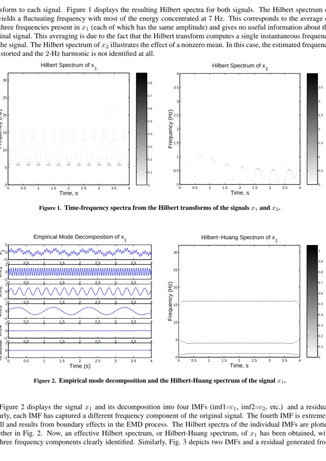
transform to each signal. Figure 1 displays the resulting Hilbert spectra for both signals. The Hilbert spectrum of
x1yields a fluctuating frequency with most of the energy concentrated at7Hz. This corresponds to the average of
the three frequencies present inx1(each of which has the same amplitude) and gives no useful information about the
original signal. This averaging is due to the fact that the Hilbert transform computes a single instantaneous frequency for the signal. The Hilbert spectrum ofx2illustrates the effect of a nonzero mean. In this case, the estimated frequency
is distorted and the2-Hz harmonic is not identified at all.
0 0.1 0.2 0.3 0.4 0.5 0.6 0.7 0.8 Time, s Frequency (Hz) Hilbert Spectrum of x 1 0 0.5 1 1.5 2 2.5 3 3.5 4 0 5 10 15 20 25 30 0 0.5 1 1.5 2 2.5 3 3.5 Time, s Frequency (Hz) Hilbert Spectrum of x 2 0 0.5 1 1.5 2 2.5 3 3.5 4 0 0.5 1 1.5 2 2.5 3 3.5 4
Figure 1. Time-frequency spectra from the Hilbert transforms of the signalsx1andx2.
0 0.5 1 1.5 2 2.5 3 3.5 4
−5 0 5 x 1
Empirical Mode Decomposition of x1
0 0.5 1 1.5 2 2.5 3 3.5 4 −2 0 2 imf1 0 0.5 1 1.5 2 2.5 3 3.5 4 −2 0 2 imf2 0 0.5 1 1.5 2 2.5 3 3.5 4 −2 0 2 imf3 0 0.5 1 1.5 2 2.5 3 3.5 4 −2 0 2 imf4 0 0.5 1 1.5 2 2.5 3 3.5 4 −2 0 2 Time (s) residual 0 0.1 0.2 0.3 0.4 0.5 0.6 0.7 0.8 0.9 1 Time, s Frequency (Hz) Hilbert−Huang Spectrum of x1 0 0.5 1 1.5 2 2.5 3 3.5 4 0 5 10 15 20 25 30
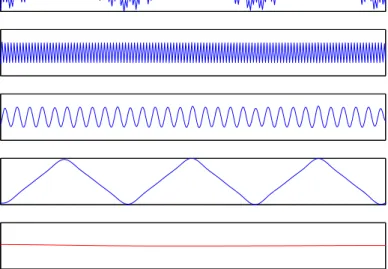
Figure 2. Empirical mode decomposition and the Hilbert-Huang spectrum of the signalx1.
Figure 2 displays the signal x1 and its decomposition into four IMFs (imf1=c1, imf2=c2, etc.) and a residual.
Clearly, each IMF has captured a different frequency component of the original signal. The fourth IMF is extremely small and results from boundary effects in the EMD process. The Hilbert spectra of the individual IMFs are plotted together in Fig. 2. Now, an effective Hilbert spectrum, or Hilbert-Huang spectrum, ofx1 has been obtained, with
0 0.5 1 1.5 2 2.5 3 3.5 4 −5
0 5
x 2
Empirical Mode Decomposition of x 2 0 0.5 1 1.5 2 2.5 3 3.5 4 −2 0 2 imf1 0 0.5 1 1.5 2 2.5 3 3.5 4 −2 0 2 imf2 0 0.5 1 1.5 2 2.5 3 3.5 4 1 2 3 Time, s residual 0 0.5 1 1.5 2 2.5 Time, s Frequency (Hz) Hilbert−Huang Spectrum of x2 0 0.5 1 1.5 2 2.5 3 3.5 4 0 0.5 1 1.5 2 2.5 3 3.5 4
Figure 3. Empirical mode decomposition and the Hilbert-Huang spectrum of the signalx2.
the signalx2. The2-Hz frequency component has been sifted into the first IMF and the ramp component has been
identified as the second IMF. The mean of the signal is2, which has been separated out as the residual. The Hilbert spectrum clearly shows the 2-Hz component and estimates a low frequency for the ramp component. This occurs because the ramp is treated as part of a low frequency wave. The IMFs and Hilbert spectra in Figs. 2 and 3 illustrate that there are some minor boundary effects associated with the EMD process. Most importantly, these examples demonstrate that EMD makes it possible to apply the Hilbert transform to signals that otherwise do not admit well-behaved Hilbert transforms.
Signal
Empirical Mode Decomposition
imf1 imf2 imf3 residual Frequency Signal Mode 1 Time Frequency Mode 2 Time Mode 3 Time Time
Figure 4. Empirical mode decomposition (EMD) and the Hilbert-Huang spectrum of the sum of two sinusoidal frequency modulations (FMs) and one Gaussian wave packet. Original signal (top), FM1, FM2, Gaussian wave packet, and residual.
Finally, two more examples20illustrate automatic and adaptive (signal-dependent) time-variant filtering of general mixtures of signals. A signal composed of three components which significantly overlap in time and frequency is
Signal
Empirical Mode Decomposition
imf1
imf2
imf3
residual
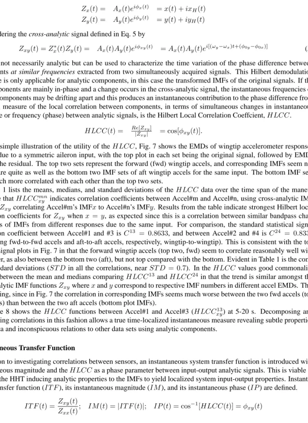
Figure 5. Empirical mode decomposition of the sum of one sinusoid with two triangular waveforms. Original signal (top), high-frequency triangular, sinusoid, low-frequency triangular, and residual.
successfully decomposed in Fig. 4 for the sum of two sinusoidal frequency modulations and one Gaussian wave packet. Another example, accenting the nonharmonic nature of EMD, is given in Fig. 5. The analyzed signal (top) is the sum of three components, a sinusoid superimposed on two triangular waveforms with periods smaller and larger than the sinusoid. The decomposition performed by the EMD is given in the three IMFs and the residue. In this case, both linear (sinusoid) and nonlinear (triangular) oscillations are effectively identified and separated. Harmonic analysis (Fourier, Morlet wavelets) would produce a less succinct and more nondescriptive decomposition.
Filtering Properties
The filtering properties of EMD have been studied in some detail.6, 7, 24 The EMD process yields a data-dependent
decomposition that focuses on local characteristics of the signal. In particular, EMD sifts out the highest-frequency component in the signal at any given time. Indeed, EMD has surprisingly been shown to behave as a dyadic bandpass filter when decomposing Gaussian white noise, much like a multiresolution wavelet decomposition. However, the EMD method as an equivalent dyadic filter bank is only in the sense of its global behavior over the entire time extent. In representing the time-frequency distribution, the Hilbert spectrum of each IMF is actually localized at any time. This is different from predetermined filtering such as with Morlet wavelet filtering.
Analytical Interpretation
The EMD is faced with the fundamental difficulty of not admitting an analytical definition, but of rather being defined by the algorithm itself, thus making the analysis of its performance and limitations difficult. The need for rigorous mathematical foundation is imperative. This fundamental problem of the empirical mode decomposition has to be resolved since only with the intrinsic mode function can nonlinear distorted waveforms be resolved from nonlinear processes. There have been attempts to circumvent the mathematical difficulties in the EMD with some success by casting the IMFs in terms of B-splines,3 and applying towards mechanical system fault-detection.15 System
identi-fication of the IMFs as a multi-component system is suggestive in the light of multiresolution system identiidenti-fication procedures such as multiresolution singular value decompositions, Kalman filters, and subspace algorithms.
More significantly, characterization of IMFs as solutions to certain self-adjoint ordinary differential equations is demonstrated.21, 22 Construction of envelopes which do not rely on the Hilbert transform is used directly to compute
the coefficients of the differential equations. These equations are natural models for linear vibrational problems and provide further insight into both the EMD procedure and utilizing its IMF components to identify systems of differen-tial equations naturally associated with the components. One of the uses of the EMD procedure is to study solutions to differential equations, and vibration analysis was a major motivation in the development of the Sturm-Liouville theory.
Hilbert Transform and Instantaneous Frequency
The Hilbert transform of a time-domain function or signalxis defined in Eq. 3,
y(t) =H{x(t)}= 1 πPV Z ∞ −∞ x(τ) t−τdτ (3)
where PV denotes the Cauchy principal value, needed because the integrand is singular atτ =t. The Hilbert transform can be viewed as the convolution of the original signal with1/t, emphasizing temporal locality ofx(t). Note that, unlike Fourier analysis, the Hilbert transform of a time-domain signal is another time-domain signal. The Hilbert transform is sometimes applied to frequency-domain signals using a similar expression as Eq. 3, but this paper will focus on the time-domain case. In practice, the Hilbert transform is usually calculated using the Fourier transform. Therefore, the fast Fourier transform algorithm can be employed for the efficient calculation of the Hilbert transform.
A signal,x, and its Hilbert transform,y, can be used to define a complex analytical signal as in Eq. 4.
z(t) =a(t)eiθ(t) =x(t) +iy(t) (4)
Therefore, the Hilbert transform pair{x(t), y(t)}can be expressed as a harmonic function with time-varying amplitude
a(t)and time-varying phase angleθ(t).
a(t) = px(t)2+y(t)2 θ(t) = tan−1 µ y(t) x(t) ¶
Given the time-dependent phase angle, the instantaneous frequency of the signal can be defined as5
ω(t) =dθ(t)
dt .
In the context of Eq. 3 with instantaneous frequency, the Hilbert transform of an IMF can be interpreted as giving the best fit with a sinusoidal function to the data weighted by1/t. Instantaneous frequency can be computed using the derivative definition or centralized finite difference.5 In general, there are an infinite number of ways to express a
signal as in Eq. 4, so there can also be an infinite number of instantaneous frequencies. The Hilbert-transform pair was proposed to uniquely define the amplitude and phase by building the complex analytic signal from the given signal with the original signal,x(t), as the real part and the orthogonal transformed signal,y(t), the imaginary part, out of phase withx(t)by π2. Note that Fourier analysis yields the decomposition
x(t) = ∞
X
j=0 ajeiωjt
which is similar to the form of the Hilbert transform in Eq. 4. A key difference, however, is that the Fourier de-composition is in terms of harmonics with constant amplitudes and frequencies. In contrast, the Hilbert transform yields instantaneous amplitudes and frequencies. Therefore, in principle, the Hilbert transform is an ideal tool for the time-frequency analysis of a general class of signals, including nonstationary signals.
Another important distinction between Fourier analysis and the Hilbert transform is that the Fourier decomposition is in terms of multiple harmonics of constant amplitude and frequency, thereby producing artificial harmonics to maintain energy conservation for nonstationary and nonlinear data. In contrast, the Hilbert transform of a signal yields an expression in terms of a single harmonic with a time-varying frequency and amplitude. For this reason, the Hilbert transform is only suitable for the analysis of mono-component signals, or signals that are composed of a single frequency component at any instant in time. This is a considerable limitation as it implies that the Hilbert transform cannot be directly applied to signals that are composed of multiple harmonics. As was shown, the Hilbert transform fails to identify the individual frequencies and instead computes a single instantaneous frequency that corresponds to a weighted average of the component frequencies. The resulting instantaneous frequency is both physically invalid and erroneous4since a multi-component signal has more than one instantaneous frequency. An additional limitation
of the Hilbert transform is that it yields extremely distorted estimates of the instantaneous frequencies of signals with nonzero mean and signals that have more local extrema than zero crossings.
The EMD responds to the dilemma surrounding the applicability of instantaneous frequency. It decomposes a multi-component signal into its associated mono-components while not obscuring or obliterating the physical essen-tials of the signal and allows the traditional definition of instantaneous frequency to be complete by being applicable to signals of both mono- and multi-component. To follow the true frequency evolution within a multi-component signal, it is necessary to break down the components into individual and physically meaningful intrinsic parts. The adaptive and nonarbitrary decomposition using EMD produces an orthogonal set of intrinsic components each retaining the true physical characteristics of the original signal. The mono-components or intrinsic modes satisfy the conditions for a well-defined notion of instantaneous frequency. These conditions include symmetry, no dependence on predefined time scales, revelation of the nature of simultaneous amplitude and phase variation, and near-orthogonality.
Finally, since instantaneous frequency displays frequency variation with time, changes of dynamic states indica-tive of nonlinearity can be identified. For example, if the instantaneous frequency of a new mode is about half of the frequency of the old mode in a bifurcation, period doubling occurs. If the instantaneous frequency of the new mode is disproportionate with the old mode, quasi-periodic bifurcation occurs. Similarly, intermittence and chaotic motion can be determined. A dynamic state can be diagnosed simultaneously by observing the changes in time of the instanta-neous frequency components and their corresponding energy. In summary, the concept of mode defined in relation to instantaneous frequency as a periodic-modal structure in the instantaneous time-frequency plane is found to be more appropriate than artificial sinusoidal harmonics in characterizing nonlinear responses.25 Instantaneous frequency is a
quantity critical for understanding nonstationary and nonlinear processes.
Local On-Line Decompositions
In the original EMD formulation, sifting iterations are applied to the predefined full length signal as long as there exists a locality at which the mean of the upper and lower envelopes is not considered sufficiently small enough. Excessive iterations on the entire signal to achieve a better local approximation contaminates other parts of the signal by overcompressing the amplitude and overdecomposing it by spreading out its components over adjacent intrinsic modes, i.e., overiteration leads to overdecomposition. The various stoppage criteria (to fulfill that the number of extrema and the number of zero crossings must differ at most by one, and that the mean between the upper and lower envelopes must be close to zero) are attempts to avoid the rigor of the symmetry of the envelopes without a mathematically rigorous definition for an adaptive basis. The hierarchical and nonlinear nature of the EMD algorithm will not provide that the EMD of segmented signals will be the segmentation of individual EMDs. Therefore, a variation referred to as local EMD20 introduces an intermediate step in the sifting process. Localities at which the
error remains large are identified and isolated, and extra iterations are applied only to them. This is achieved by introducing a weighting function such that maximum weighting is on those connected segments above a threshold amplitude, with a soft decay to zero outside those supports, much like soft-thresholding is done in wavelet denoising. Another option is based on the idea that sifting relies on interpolations between extrema, and thus only requires a finite number of them (five minima and five maxima in the case of the recommended cubic splines3, 8) for local
This led to the development of the on-line EMD.20A prerequisite for the sliding window extraction of a mode is to
apply the same number of sifting steps to all blocks in order to prevent possible discontinuities. Since this would require the knowledge of the entire signal, the number of sifting operations is proposed to be fixed a priori to a number less than 10 for effective application of the on-line version of the EMD algorithm operating in coordination with the local EMD described above. The leading edge of the window progresses when new data become available, whereas the trailing edge progresses by blocks when the stopping criterion is met on a block. Therefore, an IMF and corresponding residual are computed sequentially, then again applied to this residual, thus extracting the next mode with some delay. An aileron command multisine input used on the F/A-18 AAW for aeroservoelastic response and flutter clear-ance is shown in Fig. 6 (top plots) using the standard EMD (left) and local/on-line version (right). The bandpass nature of IMFs6, 7, 24 is reflected in the three standard IMF mean frequencies,{23.9,16.3,7.7}Hz for each of IMFs
{#1,#2,#3}, respectively, and on-line corresponding IMF mean frequencies{23.6,13.0,7.2}Hz. Immediately no-ticeable is the more efficient extraction of the signal components by the local/on-line algorithm, most evident by the sparse second and third IMFs (imf2 and imf3) being more sparse than the corresponding standard IMFs. Besides the obvious advantage of an on-line algorithm for decomposing data, it has been found to clearly surpass the standard global algorithm in terms of computational burden, especially with long original data records. An added bonus is that it generally has better orthogonality properties among the IMFs, witnessed by an order of magnitude improvement in the orthogonality index defined in Eq. 2.
Signal
EMD (constant plot scales)
imf1 imf2 imf3 0 5 10 15 20 25 30 35 Time, s residual Signal
EMD (constant plot scales)
imf1 imf2 imf3 0 5 10 15 20 25 30 35 Time, s residual
Figure 6. Standard (left) and local/on-line (right) empirical mode decomposition of an F/A-18 AAW multisine aileron com-mand input, with original signal at top and residual at bottom.
Local Analytic Signal Correlation
Since the IMFs allow permissible, meaningful, physically sensible, and unique interpretations of instantaneous frequency of general signals of interest, they fit into the class of asymptotic signals such that the time variation of the IMF amplitude and frequency may directly be recovered from the time variation of the amplitude and of the phase derivative of the associated analytic signal. An IMF after performing the Hilbert transform can be written as in Eq. 4. These complex components are now used for analysis of analytic data correlations1, 2between input-output and amongst spatially distributed sensor outputs. Note that these analyses are all local in nature since there are no assumptions of stationarity, and differ from classical double-time expressions1by being instantaneous.
Local Correlation Coefficient
Correlations are made between transformed IMFs of various signals given the associated complex analytic signals
Zx(t) = Ax(t)eiφx(t) =x(t) +ixH(t)
Zy(t) = Ay(t)eiφy(t) =y(t) +iyH(t)
by considering the cross-analytic signal defined in Eq. 5 by
Zxy(t) =Zx∗(t)Zy(t) = Ax(t)Ay(t)eiφxy(t) =Ax(t)Ay(t)ei[(ωy−ωx)t+(φ0y−φ0x)] (5)
which is not necessarily analytic but can be used to characterize the time variation of the phase difference between components at similar frequencies extracted from two simultaneously acquired signals. This Hilbert demodulation technique is only applicable for analytic components, in this case the transformed IMFs of the original signals. If the two components are mainly in-phase and a change occurs in the cross-analytic signal, the instantaneous frequencies of the two components may be drifting apart and this produces an instantaneous contribution to the phase difference from Eq. 5. A measure of the local correlation between components, in terms of simultaneous changes in instantaneous amplitude or frequency (phase) between analytic signals, is the Hilbert Local Correlation Coeffcient,HLCC.
HLCC(t) = Re[Zxy]
|Zxy| = cos[φxy(t)].
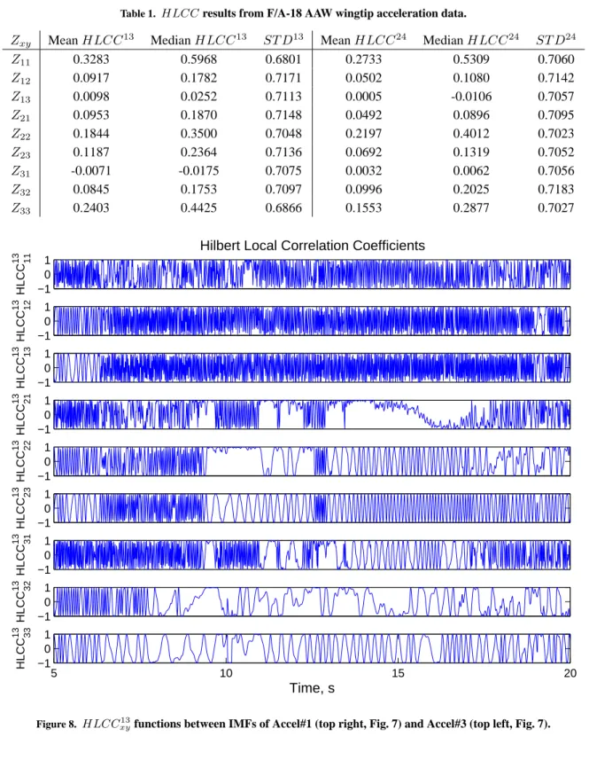
As a simple illustration of the utility of theHLCC, Fig. 7 shows the EMDs of wingtip accelerometer responses (accels) due to a symmetric aileron input, with the top plot in each set being the original signal, followed by EMDs 1-3 and the residual. The top two sets represent the forward (fwd) wingtip accels, and corresponding IMFs seem not to compare quite as well as the bottom two IMF sets of aft wingtip accels for the same input. The bottom IMF sets seem much more correlated with each other than the top two sets.
Table 1 lists the means, medians, and standard deviations of the HLCC data over the time span of the maneu-ver. Note thatHLCCmn
xy indicates correlation coefficients between Accel#m and Accel#n, using cross-analytic IMF
functionZxycorrelating Accel#m’s IMFxto Accel#n’s IMFy. Results from the table indicate strongest Hilbert local
correlation coefficients forZxy whenx= y, as expected since this is a correlation between similar bandpass
char-acteristics of IMFs from different responses due to the same input. For comparison, the standard statistical signal correlation coefficient between Accel#1 and #3 isC13 = 0.8633, and between Accel#2 and #4 isC24 = 0.8332
(correlating fwd-to-fwd accels and aft-to-aft accels, respectively, wingtip-to-wingtip). This is consistent with the top original signal plots in Fig. 7 in that the forward wingtip accels (top two, fwd) seem to correlate reasonably well with each other, as also between the bottom two (aft), but not top compared with the bottom. Evident in Table 1 is the com-mon standard deviations (ST Din all the correlations, nearST D = 0.7). In theHLCC values good commonality is found between the mean and medians comparingHLCC13andHLCC24in that the trend is similar amongst the cross-analytic IMF functionsZxywherexandycorrespond to respective IMF numbers in different accel EMDs. This
is surprising, since in Fig. 7 the correlation in corresponding IMFs seems much worse between the two fwd accels (top plot IMFs) than between the two aft accels (bottom plot IMFs).
Figure 8 shows the HLCC functions between Accel#1 and Accel#3 (HLCC13
xy) at 5-20 s. Decomposing and
representing correlations in this fashion allows a true time-localized instantaneous measure revealing subtle properties in the data and inconspicuous relations to other data sets using analytic components.
Instantaneous Transfer Function
In addition to investigating correlations between sensors, an instantaneous system transfer function is introduced with instantaneous magnitude and theHLCCas a phase parameter between input-output analytic signals. This is viable in terms of the HHT inducing analytic properties to the IMFs to yield localized system input-output properties. Instanta-neous transfer function (IT F), its instantaneous magnitude (IM), and its instantaneous phase (IP) are defined.
IT F(t) =Zxy(t)
Zxx(t); IM(t) =|IT F(t)|; IP(t) = cos
−1[HLCC(t)] =φ xy(t)
Signal
EMD for Accel#3 (left−fwd)
imf1 imf2 imf3 0 5 10 15 20 25 30 35 Time, s residual Signal
EMD for Accel#1 (right−fwd)
imf1 imf2 imf3 0 5 10 15 20 25 30 35 Time, s residual Signal
EMD for Accel#4 (left−aft)
imf1 imf2 imf3 0 5 10 15 20 25 30 35 Time, s residual Signal
EMD for Accel#2 (right−aft)
imf1 imf2 imf3 0 5 10 15 20 25 30 35 Time, s residual
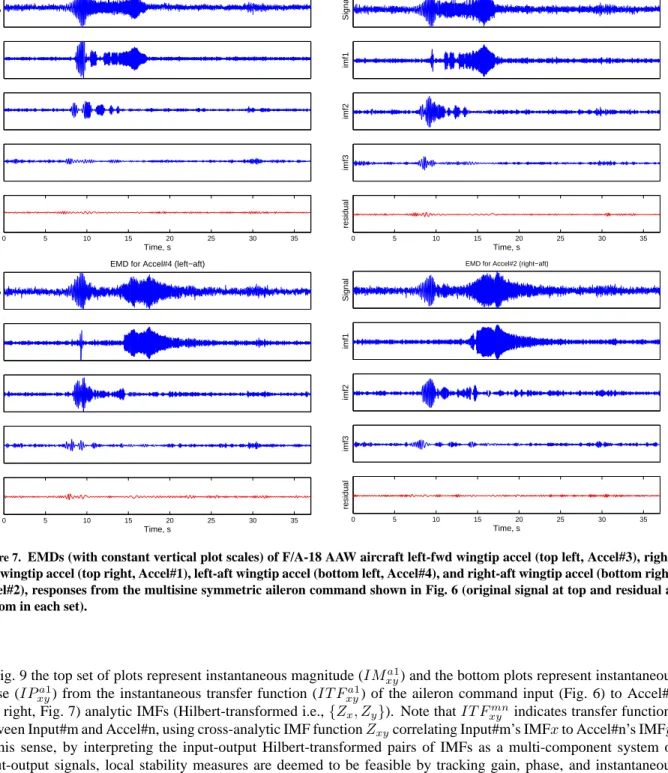
Figure 7. EMDs (with constant vertical plot scales) of F/A-18 AAW aircraft left-fwd wingtip accel (top left, Accel#3), right-fwd wingtip accel (top right, Accel#1), left-aft wingtip accel (bottom left, Accel#4), and right-aft wingtip accel (bottom right, Accel#2), responses from the multisine symmetric aileron command shown in Fig. 6 (original signal at top and residual at bottom in each set).
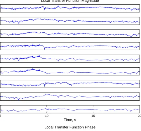
In Fig. 9 the top set of plots represent instantaneous magnitude (IMxya1) and the bottom plots represent instantaneous phase (IPxya1) from the instantaneous transfer function (IT Fxya1) of the aileron command input (Fig. 6) to Accel#1 (top right, Fig. 7) analytic IMFs (Hilbert-transformed i.e.,{Zx, Zy}). Note thatIT Fxymnindicates transfer functions
between Input#m and Accel#n, using cross-analytic IMF functionZxycorrelating Input#m’s IMFxto Accel#n’s IMFy.
In this sense, by interpreting the input-output Hilbert-transformed pairs of IMFs as a multi-component system of input-output signals, local stability measures are deemed to be feasible by tracking gain, phase, and instantaneous frequencies between each IMF pair. How these local IMF properties correspond to global system properties, given the analytic transformed IMFs, and aeroelastic and aeroservoelatic applications in stability and health monitoring, is currently being researched.
Table 1. HLCCresults from F/A-18 AAW wingtip acceleration data.
Zxy MeanHLCC13 MedianHLCC13 ST D13 MeanHLCC24 MedianHLCC24 ST D24
Z11 0.3283 0.5968 0.6801 0.2733 0.5309 0.7060 Z12 0.0917 0.1782 0.7171 0.0502 0.1080 0.7142 Z13 0.0098 0.0252 0.7113 0.0005 -0.0106 0.7057 Z21 0.0953 0.1870 0.7148 0.0492 0.0896 0.7095 Z22 0.1844 0.3500 0.7048 0.2197 0.4012 0.7023 Z23 0.1187 0.2364 0.7136 0.0692 0.1319 0.7052 Z31 -0.0071 -0.0175 0.7075 0.0032 0.0062 0.7056 Z32 0.0845 0.1753 0.7097 0.0996 0.2025 0.7183 Z33 0.2403 0.4425 0.6866 0.1553 0.2877 0.7027 −1 0 1 HLCC 13 11
Hilbert Local Correlation Coefficients
−1 0 1 HLCC 13 12 −1 0 1 HLCC 13 13 −1 0 1 HLCC 13 21 −1 0 1 HLCC 13 22 −1 0 1 HLCC 13 23 −1 0 1 HLCC 13 31 −1 0 1 HLCC 13 32 5 10 15 20 −1 0 1 HLCC 13 33 Time, s
−50 0 50 IM 11 , dB
Local Transfer Function Magnitude
−50 0 50 IM 12 −50 0 50 IM 13 −50 0 50 IM 21 −50 0 50 IM 22 −50 0 50 IM 23 −50 0 50 IM 31 −50 0 50 IM 32 5 10 15 20 −50 0 50 IM 33 Time, s 0 100 200 IP11 , deg
Local Transfer Function Phase
0 100 200 IP 12 0 100 200 IP 13 0 100 200 IP21 0 100 200 IP22 0 100 200 IP 23 0 100 200 IP 31 0 100 200 IP 32 5 10 15 20 0 100 200 IP33 Time, s
Figure 9. Instantaneous log-magnitude (IMa1
xy, top plot set) and phase (IPxya1, bottom plot set) of IMF transfer functions
Empirigrams and Empirical Local Correlation Coefficient
Given two EMDs from different signals, select a common number of IMFs to use for correlation (as three were selected in earlier examples for input and outputs). This is generally not difficult, especially for aeroelasticity data, since the higher-numbered IMFs approach a residual characteristic quickly. From the transformed IMFs,{Zx(t), Zy(t)},
define the corresponding set of two-dimensional Hilbert empirigrams,{Hx(ηx, t), Hy(ηy, t)}, where for each common
η =ηx =ηy, the IMF number from the input EMD corresponds with the output EMD. Define in Eq. 6 the Hilbert cross-empirigram
Hxy(η, t) =Hx∗(η, t)Hy(η, t) (6)
which correlates the respective IMFs from the two Hilbert empirigrams. Empirigrams relate to time-scale wavelet scalograms,5which relate to time-frequency maps, since scales relate to frequencies in standard wavelet
decomposi-tions. Because of the bandpass nature of IMFs discussed previously, a similar construction emanates with the HHT. As with wavelet scalograms, the real part of the cross-empirigram (co-empirigram) gives the instantaneous contribution of each IMF to the correlation between two signals. An Empirical Local Correlation Coefficient,ELCC(η, t), is then defined as
ELCC(η, t) = Re[Hxy(η,t)] |Hxy(η,t)| =
Re[Hxy(η, t)] |Hx(η, t)||Hy(η, t)|
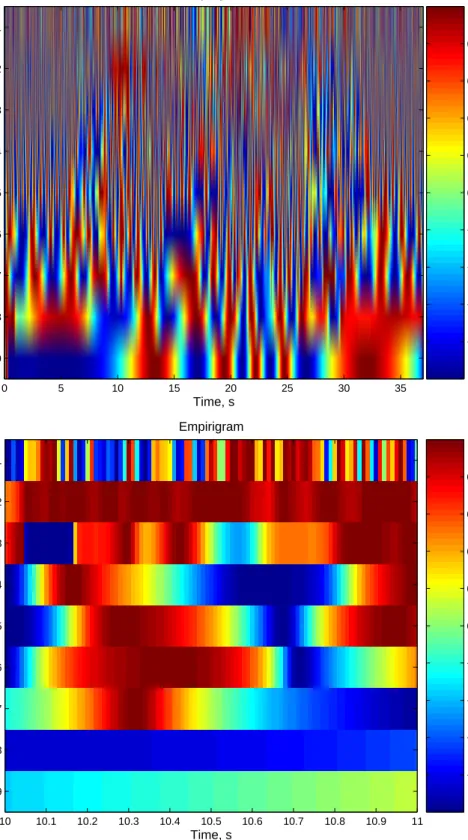
whereELCC(η, t)(between±1, as theHLCC) gives the instantaneous contribution between corresponding IMFs from the two signals to the correlation coefficient. Figure 10 shows an imaged decomposition plot of theELCC between the input signal from Fig. 6 to Accel#1 in Fig. 7, but includes all nine IMFs from the EMDs of the input and output. The first row represents the contributions of the first input IMF to first output IMF, etc., up to the ninth IMF. In each IMF row there is much oscillation (higher frequency in the first and lower frequency to the ninth) of contributions from corresponding IMFs to the correlation. There are generally stronger correlations over longer time spans in the higher-numbered IMFs (lower frequencies), but the lower-numbered IMF correlations are less obvious due to the higher frequency content. There is a tendency to cycle from high-to-low-to-high [strong(positive)-to-none-to-strong(negative)] correlation very rapidly. A more detailed depiction in the zoomed-in bottom plot, between 10-11 s, demonstrates a rich interplay between correlation of mid-to-lower IMFs (higher frequencies) over the shorter time period. Yet another view is presented in Fig. 11, where the contours are split up discretely in three dimensions showing the heavy emphasis in the higher frequencies because the contours are more congested in each of the IMF levels. These representations highlight the areas of commonality and incongruity between corresponding input-output IMFs.
From the Hilbert spectrumH(ω, t)the energy spectrumH2(ω, t)gives instantaneous energy,
IE(t) =
Z
ω
H2(ω, t)dω
which is an indication of the energy fluctuations with time being weighted by the Hilbert spectrum localized energy over the entire set of IMFs. Corresponding to the signals in Fig. 7 are the instantaneous energy profiles of the output accelerometer responses in Fig. 12 (top set of four plots). The aft wingtip accels (bottom plots) are very similar (from the symmetric aileron input), indicating energy at{7−10,13−20,30}s time locations. In this case, with the particular multisine input from Fig. 6 programmed over the3−35Hz frequency range, these times correspond closely to the primary F/A-18 AAW modal frequencies in a corresponding frequency range, i.e.,{6−9,12−20,30−35}Hz, as will be shown with marginal Hilbert spectra. The forward accelerometer responses in the top plots are also very similar indicating modes near{6,12−17,25−32}Hz. Instantaneous energy over a sensor suite is therefore a nonstationary indicator of time-varying energy distribution amongst the sensor array.
Marginal Spectra
From the Hilbert spectrumH(ω, t), the marginal spectrum is also defined.
h(ω) =
Z
t
Time, s IMF Number Empirigram 0 5 10 15 20 25 30 35 1 2 3 4 5 6 7 8 9 −0.8 −0.6 −0.4 −0.2 0 0.2 0.4 0.6 0.8 Time, s IMF Number Empirigram 10 10.1 10.2 10.3 10.4 10.5 10.6 10.7 10.8 10.9 11 1 2 3 4 5 6 7 8 9 −0.8 −0.6 −0.4 −0.2 0 0.2 0.4 0.6 0.8
Figure 10. Empirical local correlation coefficientELCC plots using two different representations of theELCC between the input signal from Fig. 6 to Accel#1 in Fig. 7. Top plot is an intrinsic mode component-by-component depiction, starting
0 10 20 30 2 4 6 8 −0.8 −0.6 −0.4 −0.2 0 0.2 0.4 0.6 0.8 ELCC Empirigram Time, s IMF Number −0.8 −0.6 −0.4 −0.2 0 0.2 0.4 0.6 0.8
0 10 20 30 40 −50 0 50 IE, dB Accel#1 0 10 20 30 40 −50 0 50 Time, s IE, dB Accel#2 0 10 20 30 40 −50 0 50 IE, dB Accel#3 0 10 20 30 40 −50 0 50 Time, s IE, dB Accel#4 0 10 20 30 40 −150 −100 −50 0 Magnitude, dB Accel#1 0 10 20 30 40 −150 −100 −50 0 Frequency, Hz Magnitude, dB Accel#2 0 10 20 30 40 −150 −100 −50 0 Magnitude, dB Accel#3 0 10 20 30 40 −150 −100 −50 0 Frequency, Hz Magnitude, dB Accel#4
Figure 12. Instantaneous energy (top plot set) and marginal spectra (bottom plot set) of right-fwd wingtip accel (top right, Accel#1), right-aft wingtip accel (bottom right, Accel#2), left-fwd wingtip accel (top left, Accel#3), and left-aft wingtip accel
Corresponding to the signals in Fig. 7 are the marginal spectra of the output accelerometer responses in Fig. 12 (bottom set of four plots). The aft wingtip accels (bottom plots) are again similar showing modal response at{5−10,12−
20,30−35}Hz. The forward accelerometer responses in the top plots are also again very similar indicating modes near{6,12−17,25−32}Hz.
The marginal spectrum measures total amplitude (or energy) contributions from each frequency value over the entire data record in a probabilistic sense. Frequency in eitherH(ω, t)orh(ω)is very different from Fourier spectral analysis. In the Fourier analysis the existence of energy at a frequency implies a wave component persisting through the data. Energy at the marginal Hilbert frequency, however, implies a higher likelihood (expected value over time) for such a wave to have appeared locally. As stated earlier, the Hilbert transform of an IMF gives the best fit with a sinusoidal function to the data weighted by 1/t, which makes it instantaneous. In fact, the Hilbert spectrum is a weighted nonnormalized joint amplitude-frequency-time distribution in which the weight assigned to each time-frequency cell is the local amplitude. Consequently, time-frequency in the marginal spectrum indicates only the likelihood that an oscillation with such a frequency exists. Exact occurrence of frequency content is given in the full Hilbert spectrum. The Fourier spectrum is meaningless for nonstationary data, and there is little similarity between Hilbert and Fourier from previous studies8, 9 for nonstationary data. Also, marginal cross-spectra between signals does not
make sense since the time-dependence (causality) is lost and the frequencies are time-ignorant, so an input-output correlation at a certain frequency is meaningless.
The time-frequency Fourier spectrum, a spectrogram, suffers from the same restrictions over time due to window-ing distortions. There is a lower bound on the local time-frequency resolution uncertainty product of the spectrogram due to the windowing operation. This limitation is an inherent property of the spectrogram and is not a property of
the signal or a fundamental limit.17 For many other time-frequency distributions, the local uncertainty product is less than that of the Fourier spectrogram and can be arbitrarily small. These results are contrary to the common notion that the uncertainty principle limits local quantities. Similar considerations apply to window-based filter bank (wavelet) methods. This limitation is due to the window and not to any inherent property of the signal.
This is a key point for application and understanding of HHT analysis, that windowing is not a factor, so standard time-frequency resolution limitations based on the uncertainty principle do not apply. As seen in the on-line analysis, an adaptive sliding window method has good performance simply requiring adequate data in the window to initiate a sifting process for satisfying the two IMF properties for analyticity.
Wing Dynamics Analysis
Dynamics between different sensors from the same input will now be investigated. This information will be used to guide the analysis of a group of wing accelerometer responses from a single input in terms of input-output correlation contribution for the F/A-18 AAW aircraft18and Aerostructures Test Wing (ATW).12
F/A-18 Active Aeroelastic Wing (AAW) Aircraft
Collective F/A-18 AAW aileron position, used as the multisine input, was obtained as the average of four position transducer measurements from the right and left ailerons. Outputs are twelve wing structural accelerometers located at the left (six accels) and correponding right (six accels) outer wings, all sampled at 400 sps, as designated in Table 2. EMDs were calculated for the input and all outputs, with mean frequencies calculated for all the output IMFs compared to the single input IMFs. Table 3 is a summary of the results. Included are the first six IMFs averaged amongst the accels, percentage differences of these compared to the input IMFs, and standard deviations of output sensor IMFs. The accels correspond very well amongst each other in IMF frequencies (as frequency decreases, from left to right). The comparison to the input frequency is excellent even though input and output EMDs are performed independently. Orthogonality of the IMFs in each case was also very good. This shows that for this type of data, where responses are all from a common input (whether it is known or not), IMFs can be used for sensor-to-sensor correlation and input-output analysis.
Now the concept of the using the essentially-orthogonal analytic IMFs from the inputs and outputs is pursued to establish a multi-loop connotation of input IMFs to output IMFs for correlation and even stability properties. The
Table 2. F/A-18 AAW wing accelerometer nomenclature.
3. L-wt-fwd 1. R-wt-fwd
3. Left-wingtip forward 1. Right-wingtip forward
7. L-wof-fwd 5. R-wof-fwd
7. Left-wing outer-fold forward 5. Right-wing outer-fold forward
11. L-wif-fwd 9. R-wif-fwd
11. Left-wing inner-fold forward 9. Right-wing inner-fold forward
4. L-wt-aft 2. R-wt-aft
4. Left-wingtip aft 2. Right-wingtip aft
8. L-wof-aft 6. R-wof-aft
8. Left-wing outer-fold aft 6. Right-wing outer-fold aft 12. L-wif-aft 10. R-wif-aft 12. Left-wing inner-fold aft 10. Right-wing inner-fold aft
Table 3. IMF frequencies from F/A-18 AAW input collective aileron position and outer wing response data.
Signal IMF1 IMF2 IMF3 IMF4 IMF5 IMF6
0. Input 116.62 59.61 29.34 16.75 9.05 4.90 1. R-wt-fwd 99.05 56.94 27.90 12.56 6.96 3.62 2. R-wt-aft 123.85 71.36 35.15 16.83 9.35 5.02 3. L-wt-fwd 114.47 66.05 33.78 15.06 7.95 5.32 4. L-wt-aft 127.56 78.71 41.73 21.06 11.92 6.58 5. R-wof-fwd 105.83 58.52 32.06 17.17 9.34 5.47 6. R-wof-aft 96.31 54.96 29.24 14.91 8.64 4.63 7. L-wof-fwd 115.93 58.77 30.88 16.59 8.66 4.32 8. L-wof-aft 102.99 52.76 27.14 15.35 8.65 4.83 9. R-wif-fwd 112.19 60.61 31.99 17.78 9.90 5.17 10. R-wif-aft 115.39 64.07 36.09 19.05 10.29 5.72 11. L-wif-fwd 124.91 66.06 32.99 18.32 10.53 5.19 12. L-wif-aft 129.41 66.05 34.02 17.97 9.66 4.92
Average Output IMF Frequencies
Absolute 114.0 62.9 32.8 16.9 9.3 5.1
Wrt Input 2.3% 5.2% 10.4% 0.8% 2.9% 3.2% Output IMF Frequency STDs
Absolute 11.2 7.3 4.0 2.2 1.3 0.7
Wrt Mean 9.8% 11.7% 12.1% 13.2% 13.9% 14.4%
input IMFs are interpreted as an orthogonal decomposition of the input(s), and the same for output IMFs for out-put(s). This can be generalized to multi-input-multi-output (MIMO) signal analysis where in reality each signal is represented by its EMD. Recall from the transformed input-output IMFs,{Zx(t), Zy(t)}, the corresponding set of
input and output EMDs. For the analysis described here it is not necessary to use an identical number,η, of IMFs from input and output (but this restriction is maintained here for simplicity). Then the Hilbert cross-empirigram
Hxy(η, t) =Hx∗(η, t)Hy(η, t)correlates the respective analytic IMFs from the two Hilbert empirigrams. Now define
σxy(η) = σ[Hx∗(η, t)HyT(η, t)]
whereσxyrepresents theη-vector of singular values from the singular value decomposition (SVD) of the product of the
empirigrams. The singular values represent relative contributions from the principal cross-correlation analytic IMFs as a result of correlation of all input analytic IMFs to all output analytic IMFs over the entire time span. Therefore, higher
σ-valued cross-analytic IMFs have more input-output significance in terms of operator norm from input to output. The maximum singular value,σ¯xy = maxη(σxy(η)), of this input-output operator corresponds to the structured singular
value with a full-complex uncertainty block structure. In this context, forMηxη = Hx∗(η, t)HyT(η, t), a complex matrix operator of input analytic IMFs to output analytic IMFs, µ∆(M) is a measure of the smallest uncertainty
∆ =Cηxη(note that ifη
x6=ηy, then∆ = Cηyxηx is not square) that causes instability if interpreted as a constant
matrix feedback loop,30
µ{∆=Cηxη}(M) = σ¯[Hx∗(η, t)HyT(η, t)]
and for scalar uncertainty structure∆ ={δIη:δ∈C}representing diagonal structure between input-output IMFs,
µ∆(M) = ρ[Hx∗(η, t)HyT(η, t)]
whereρis the spectral radius (largest magnitude eigenvalue). This is distinctly different from the full-block structure in that uncertainty is only between corresponding input-output analytic IMFs (similar dominant frequencies), while ignoring uncertainty across different analytic IMFs (of different dominant frequencies) between input and output. This is obviously less conservative but generally less realistic as well, especially for nonlinear effects which cross frequencies. Largerµ∆values in either case represent effects of uncertainty between input and output such that higher
correlated IMFs relate to more sensitivity to uncertainty at those dominant IMF frequencies.
For MIMO signal analysis, it would be most appropriate to combine complex blocks (either full or scalar) for each input-output into a multi-block structure, where each complex sub-block corresponds to an input-output analytic IMF complex uncertainty structure. In computation this is often expanded in a block-diagonal context with repeated scalar and full blocks,30 where in this case each of these blocks would correspond to a single input-output analytic IMF uncertainty structure.
Table 4. Normalizedµ∆results from F/A-18 AAW left and right wing acceleration data.
Full 3. L-wt-fwd 7. L-wof-fwd 11. L-wif-fwd 9. R-wif-fwd 5. R-wof-fwd 1. R-wt-fwd Block 4. L-wt-aft 8. L-wof-aft 12. L-wif-aft 10. R-wif-aft 6. R-wof-aft 2. R-wt-aft
Fwd-wing 0.29 0.29 0.73 1.00 0.62 0.80
Aft-wing 0.65 0.67 0.56 0.19 0.31 0.72
Scalar 3. L-wt-fwd 7. L-wof-fwd 11. L-wif-fwd 9. R-wif-fwd 5. R-wof-fwd 1. R-wt-fwd Block 4. L-wt-aft 8. L-wof-aft 12. L-wif-aft 10. R-wif-aft 6. R-wof-aft 2. R-wt-aft
Fwd-wing 0.11 0.13 0.19 1.00 0.47 0.49
Aft-wing 0.23 0.42 0.27 0.11 0.06 0.34
To compare input-to-output correlations from aileron position to wing accels for different uncertainty structures, structured singular values were computed for the full-block and scalar-block structures between the collective aileron position and F/A-18 AAW wing accelerometer responses, then normalized with respect to the largest of the group. Table 4 lists the results for both types of uncertainty structures. Accelerometer#9 has the highest correlation (=1.00) with the input aileron position in either case. Interestingly, comparison between left and right wing accels is poor
0 10 20 30 40 −40
−20 0
1.R−wt−fwd
AAW Wing Accels
0 10 20 30 40 −40 −20 0 2.R−wt−aft Mu, g/deg (dB) 0 10 20 30 40 −40 −20 0 3.L−wt−fwd 0 10 20 30 40 −40 −20 0 4.L−wt−aft 0 10 20 30 40 −40 −20 0 5.R−wof−fwd 0 10 20 30 40 −40 −20 0 6.R−wof−aft 0 10 20 30 40 −40 −20 0 7.L−wof−fwd 0 10 20 30 40 −40 −20 0 8.L−wof−aft 0 10 20 30 40 −40 −20 0 9.R−wif−fwd 0 10 20 30 40 −40 −20 0 10.R−wif−aft 0 10 20 30 40 −40 −20 0 11.L−wif−fwd Time, s 0 10 20 30 40 −40 −20 0 12.L−wif−aft Time, s 0 10 20 30 40 −40 −20 0 1.R−wt−fwd
AAW Wing Accels
0 10 20 30 40 −40 −20 0 2.R−wt−aft Mu, g/deg (dB) 0 10 20 30 40 −40 −20 0 3.L−wt−fwd 0 10 20 30 40 −40 −20 0 4.L−wt−aft 0 10 20 30 40 −40 −20 0 5.R−wof−fwd 0 10 20 30 40 −40 −20 0 6.R−wof−aft 0 10 20 30 40 −40 −20 0 7.L−wof−fwd 0 10 20 30 40 −40 −20 0 8.L−wof−aft 0 10 20 30 40 −40 −20 0 9.R−wif−fwd 0 10 20 30 40 −40 −20 0 10.R−wif−aft 0 10 20 30 40 −40 −20 0 11.L−wif−fwd Time, s 0 10 20 30 40 −40 −20 0 12.L−wif−aft Time, s
even from a symmetric aileron input, thereby indicating asymmetry and/or nonlinearity. Lowerµ∆values indicate a
degree of robustness to uncertainty in a feedback stability sense, and as pointed out previously, scalar uncertainty is prevalently less conservative (as evidenced from absolute values before normalizing since the normalization factor is almost equal between the uncertainty structures). If an apriori bound on gain levels (normalization) between input-output is defined such thatk ∆ k∞< 1is considered acceptable in some sense (stability, health diagnostic, safety
margin), thenµ∆has an absolute (scaled) interpretation such thatµ∆>1indicates that an acceptable threshold has
been exceeded, and this can be used as a health, stability, or safety monitor.
A time-dependent interpretation is also available by calculatingµ∆(M, t)at each time point. µ∆(M, t) = ρ[Hx∗(η, ti)HyT(η, ti)]∀ti (scalar-block uncertainty structure)
= σ¯[H∗
x(η, ti)HyT(η, ti)]∀ti (full-block uncertainty structure).
In Fig. 13 are plots ofµ∆(M, t)for each input-to-output (aileron-to-accel) normalized analytic IMFs where it is evident
that values close to one (0 dB) are near a unity operator norm limit. Again, this depends on the boundk ∆ k∞< 1
indicating an acceptable threshold, in this case maximum input-to-output gain normalized to one. Values close to one (0 dB) approach the acceptable limit. This uncertainty structure application has implications for model validation in the time domain.19
Aerostructures Test Wing (ATW)
Another example which includes an actual instability is taken from Aerostructures Test Wing12(ATW) flight test data.
The input is a sine sweep PZT voltage and outputs are three wingtip accelerometer responses. The EMDs of the PZT input and center wingtip accelerometer output near the flutter condition are displayed in Fig. 14. Flutter response
Signal
EMD (constant plot scales)
imf1 imf2 imf3 0 10 20 30 40 50 60 Time, s residual Signal
EMD (constant plot scales)
imf1 imf2 imf3 0 10 20 30 40 50 60 Time, s residual
Figure 14. Empirical mode decomposition of the ATW input PZT (left plot) and center wingtip accelerometer (right plot) at Mach 0.82, 10,000 feet (3,048 m) altitude, just before flutter (original signal at top and residual at bottom in each set).
EMDs of the center wingtip accelerometer and correspondingµ∆(M, t)plots between input analytic IMFs and all
three wingtip accelerometer output analytic IMFs are shown in Fig. 15. The input PZT was not activated during the flutter occurrence, so the input is essentially a small arbitrary oscillation about zero. It is evident that at the point of instability past 7.5 s, µ∆(M, t)appropriately approaches a value of one (0 dB) since the input and output are
normalized to unity, and assuming this limit corresponds to the limit of stability, and output response approaches its upper limit at flutter.
Signal
EMD (constant plot scales)
imf1 imf2 imf3 0 1 2 3 4 5 6 7 Time, s residual 0 1 2 3 4 5 6 7 −50 −40 −30 −20 −10 0 Fwd−Wingtip−Accel Mu, g/Volt (dB) 0 1 2 3 4 5 6 7 −40 −20 0 Mid−Wingtip−Accel Mu, g/Volt (dB) 0 1 2 3 4 5 6 7 −50 −40 −30 −20 −10 0 Aft−Wingtip−Accel Mu, g/Volt (dB) Time, s
Figure 15. Empirical mode decomposition of the center wingtip accelerometer (left plot) near Mach 0.83, 10,000 feet (3,048 m) altitude, at flutter (original signal at top and residual at bottom), and time-varyingµ∆(M, t)for full-block uncertainty between input and output IMFs of the three wingtip accelerometer outputs (right plots).
Parameter Estimation Using the Hilbert-Huang Transform
The Hilbert transform can used for estimating modal parameters such as natural frequencies and damping ratios. For a single-mode system, the damped natural frequency can be easily determined from the Hilbert transform of the impulse response function. In this case, the damped natural frequencyωdis given by the slope of the instantaneous
phase angle plotted as a function of time, and damping ratioζis estimated in a straightforward manner.23
For a linear single-mode system characterized by a pair of complex conjugate eigenvalues, the eigenvalues are directly related to the modal parameters as−ζωn+ωd, whereωndenotes the natural frequency. The impulse response
function is given by
h(t) = 1
mωd
e−ζωntsin(ω
dt)
wheremdenotes the mass. Provided the damping ratio is small, the following relationships hold23 H©e−ζωntsin(ω dt) ª = e−ζωntcos(ω dt) H©e−ζωntcos(ω dt) ª = −e−ζωntsin(ω dt)
where again H denotes the Hilbert transform. Therefore, the Hilbert transform of the impulse response function can be written as
H{h(t)}:= ˜h(t) = 1
mωd
e−ζωntcos(ω
dt).
The impulse response function can then be viewed as the real part of the following analytic signal23 z(t) = h(t) +i˜h(t) = 1 mωd e−ζωntsin(ω dt) +i 1 mωd e−ζωntcos(ω dt).
The amplitude of this signal is given by
a(t) =
q
h(t)2+ ˜h(t)2= 1
mωd
which represents the envelope of the impulse response. Taking the natural logarithm of the amplitude yields
ln (a(t)) =−ζωnt−ln (mωd).
The slopeσof the natural log ofa(t)plotted against time givesσ=−ζωn. Given thatωdcan be obtained from the
slope of the phase plotted against time, and using the definition of the damped natural frequency, there resultsωn,
ωd = p 1−ζ2ω n ω2 d = (1−ζ2)ωn2=ω2n−σ2 ωn = q ω2 d+σ2
and the damping ratio can be calculated asζ =σ/ωn. This approach to damping estimation is in the same spirit as
the logarithmic decrement technique commonly used in structural dynamics.
Most systems have multiple modes, however, which implies that the impulse response function will generally contain contributions from several modes. Therefore, because they are valid only for single-mode systems, logarithmic decrement or the approach based on the Hilbert transform cannot be used for estimating damping. As emphasized earlier, the Hilbert transform does not yield meaningful frequency information for multiple-mode systems since it attempts to identify a single instantaneous frequency at each time step. The Hilbert-Huang algorithm makes it possible to apply the above technique for damping and frequency estimation because it can decompose a multi-component signal into a series of single-component signals through the EMD process. By performing EMD on the impulse response function of a multiple-mode system, the contributions of the different modes can be extracted and analyzed separately. This approach has been applied by Yang et al.26–28 in a series of papers in which the Hilbert-Huang
algorithm was used for parameter estimation of several multiple degree-of-freedom structures. A similar analysis is used here to estimate damping ratios and frequencies for aeroelastic systems.
As an example, consider a prototypical linear pitch-plunge aeroelastic system that has been studied extensively in the literature. The system consists of an airfoil with pitch and plunge degrees of freedom, and the input is the deflectionβof the trailing edge flap. The equations of motion for this system are given by
" m mxαb mxαb Iα # ( ¨ h ¨ α ) + " ch 0 0 cα # ( ˙ h ˙ α ) + " kh 0 0 kα # ( h α ) =ρU2b clα ³ α+ 1 Uh˙ +U1 ¡1 2−a ¢ bα˙´ cmα ³ bα+ 1 Ubh˙ +U1 ¡1 2−a ¢ b2α˙´ +ρU2b " −clβ cmβb # β
wherehdenotes the plunge displacement of the airfoil andαrepresents the pitch angle. Left-hand side terms describe the structural dynamics of the system while right-hand side terms represent quasi-steady aerodynamic forces and moments. In this study, the flow velocityU is varied until the linear flutter speed is reached at approximatelyU = 11.8m/s. The values of the other system parameters are held constant as listed in Table 5.
Table 5. Parameters for the pitch-plunge aeroelastic system.
m = 12.387 kg a = -0.6 clα = 6.28 kh = 2844.4 N/m
Iα = 0.065 m2kg xα = 0.2466 cmα = -0.628 kα = 2.82 Nm
ρ = 1.225 kg/m3 ch = 27.43 kg/s clβ = 3.358
b = 0.135 m cα = 0.036 m2kg/s cmβ = -0.635
Because this system has two outputs, pitch and plunge, there are two impulse response functions that can be measured. Each of these functions generally contains contributions from both modes of the system. As an example,
0 2 4 6 8 10 12 14 16 −4 −3 −2 −1 0 1 2 3 4x 10
−4 Impulse Response, h − Plunge, U=8 m/s
Time, s Magnitude (m/rad) 0 2 4 6 8 10 12 14 16 −0.4 −0.3 −0.2 −0.1 0 0.1 0.2 0.3 0.4
Impulse Response, α − Pitch, U=8 m/s
Time, s
Magnitude (rad/rad)
Figure 16. Plunge and pitch impulse response functions forU = 8m/s
−5 0 5x 10 −4 Impulse Response −5 0 5x 10 −4 imf1 −5 0 5x 10 −4 imf2 0 5 10 15 −5 0 5x 10 −4 Time, s imf3
Fig. 16 depicts the pitch and plunge impulse response functions for a flow velocity ofU = 8m/s. These were obtained by simulating the pitch and plunge responses to an impulse applied to the trailing edge flap. The plunge impulse responses are used over a range of flow velocities to measure frequencies and damping ratios using the Hilbert-Huang algorithm. These impulse response functions are obtained by way of simulation in this paper, but in practice they can be obtained by way of system identification techniques such as taking the inverse Fourier transform of the measured frequency response function or identifying first-order Volterra kernels from measured input-output data.
0 2 4 6 8 10 12 14 16 0 20 40 60 80 100 120 140 160 180 Time, s
Phase Angle (rad)
Region I: Plunge (h) slope = ω
d=15.75 rad/s
Region II: Pitch (α) slope = ωd=8.004 rad/s 0 2 4 6 8 10 12 14 16 −20 −18 −16 −14 −12 −10 −8 −6 Time, s
Amplitude (Natural Log)
Region II: Pitch, (α) slope=−ζωn=−.4857 rad/s
Region I: Plunge (h) slope=−ζωn=−1.448 rad/s
Figure 18. Instantaneous phase and amplitude plots used to estimate modal parameters from the first IMF of the plunge impulse response function atU = 8m/s.
The plunge impulse response functions were used to estimate the damped natural frequencies, damping ratios, and natural frequencies over a range of flow velocities. The results are summarized in Table 6, which lists the actual and estimated damped natural frequencies and damping ratios for flow velocities ranging fromU = 1m/s toU = 11.9m/s (just past the linear flutter speed). The actual frequencies and damping ratios were calculated by solving for the eigenvalues of the system. The estimation of the modal parameters forU = 8m/s is demonstrated in Figs. 17 and 18. Figure 17 illustrates the EMD of the plunge impulse response function atU = 8m/s. In this case, both modes of vibration are evident in the first intrinsic mode function. This is because the first, higher-frequency mode damps out quickly and the second mode persists for a longer period of time. Therefore, the frequencies and damping ratios of both modes were estimated by using different portions of the first IMF, as depicted in Fig. 18. The figure shows plots of the instantaneous phase and the natural log of the amplitude of the first IMF. Recall that the slopes of these lines are used to estimate the modal parameters. The initial portion of the amplitude plot is not a straight line because of initial transients in the IMF and possible boundary effects. Therefore, the portions of the plot that most resembled straight lines were used for the slope calculations for each mode, as labeled in the figure. Because this analysis technique is only approximate depending on the magnitude of the damping ratio (increased error for larger damping), the amplitude curve tends to oscillate about an average slope. Therefore, the slope in each case was obtained using a linear least-squares curve-fit of the data.26–28
The results presented in Table 6 show that the estimates of the damped natural frequencies and damping ratios are fairly accurate in most cases. As the linear flutter speed (approximatelyU = 11.8 m/s) is approached, the plunge mode is not discernible in the IMFs. In this regime, the system behaves essentially as a single-mode system and it was not possible to estimate the damping and frequency of the plunge mode. The actual and estimated damping ratios for each mode are plotted as a function of flow velocity in Fig. 19.
A few observations are now presented. The first IMF was used to estimate the parameters of both modes. The analysis would be somewhat cleaner if each mode appeared in a different IMF. This is indeed the case in the work of Yang et al.26–28in which the frequency range of each IMF is controlled in the EMD process. Therefore, controlling the