Road classification for two-wheeled vehicles

This version is available at https://doi.org/10.14279/depositonce-8144

Gorges, C., Öztürk, K., & Liebich, R. (2017). Road classification for two-wheeled vehicles. Vehicle System Dynamics, 56(8), 1289–1314.

https://doi.org/10.1080/00423114.2017.1413197

This is an Accepted Manuscript of an article published by Taylor & Francis in Vehicle System Dynamics on 14 December 2017, available online:

http://www.tandfonline.com/10.1080/00423114.2017.1413197.

Gorges, C.; Öztürk, K.; Liebich, R.

Road classification for two-wheeled

vehicles

Accepted manuscript (Postprint) Journal article |

Road classification for two-wheeled vehicles Christian Gorgesa, Kemal Öztürka, Robert Liebichb

a_{BMW AG, Munich, Germany;}b_{Chair of Engineering Design and Product Reliability,} Berlin Institute of Technology, Berlin, Germany

(This is an Accepted Manuscript of an article published by Taylor & Francis in Vehicle System Dynamics on 14/12/2017, available online: http: // www. tandfonline. com/ 10. 1080/ 00423114. 2017. 1413197.)

This publication presents a three-part road classification system that util-ises the vehicle’s onboard signals of two-wheeled vehicles. First, a curve estimator was developed to identify and classify road curves. In addition, the curve estimator continuously classifies the road curviness. Second, the road slope was evaluated to determine the hilliness of a given road. Third, a modular road profile estimator has been developed to classify the road profile according to ISO 8608, which utilises the vehicle’s transfer functions. The road profile estimator continuously classifies the driven road. The proposed methods for the classification of curviness, hilliness, and road roughness have been validated with measurements. The road classification system enables the collection of vehicle-independent field data of two-wheeled vehicles. The road properties are part of the customer usage profiles which are essential to define vehicle design targets.

Keywords: Road classification, road profile estimation, ISO 8608, curve detection, customer usage profiles, motorcycle dynamics

1 Introduction

Customer usage profiles are a key factor in durability analysis and product design. The detailed knowledge of customer usage profiles improves design loads and ultimately the vehicle development process. On the one hand they are essential to define vehicle design targets as Gorges et al. [1] and Johannesson and Speckert [2] discussed. On the other hand customer usage profiles enable a virtual load acquisition, where customer loads are simulated on virtual test tracks. Johannesson and Speckert [2] highlight that the customer usage distribution consists of three components: customer usage, vehicle-independent road properties, and the vehicle model. The vehicle-vehicle-independent road prop-erties are the main focus of the present research. It has the objective to collect information about the driven road classes using the onboard signals of two-wheeled vehicles.

Common methods to obtain customer loads are survey sampling and online- monit-oring systems. Survey sampling is expensive due to extra measurement equipment and cannot reveal the entire customer load distribution. Müller [3] and Matz [4] already

developed model-based online monitoring system with integrated counting of durability-related values. This has become possible because the number of onboard sensors rises anyway due to the increased functions of motorcycles including an anti-lock braking sys-tem, dynamic traction control, or curve assistant. Onboard signals are defined as signals that can be accessed by the vehicle’s Controller Area Network (CAN) bus. In addition, Gorges et al. [1] developed a customer load acquisition system for two-wheeled vehicles that utilises the vehicle’s onboard signals to gather wheel forces and vehicle loading. As a result, customer loads are revealed that are directly associated with the fatigue of the vehicle. Hence, the loads are vehicle-dependent. On the contrary, the present research has the objective to collect vehicle-independent road properties. Karlsson [5] has already discussed methods to derive customer loads from road classification but the question remains how the distribution of road classes driven by the customers can be revealed.

Therefore, this publication presents methods to detect and evaluate road classes in terms of curviness, hilliness, and most importantly road roughness, which is evaluated in terms of ISO 8608 [6]. On the small scale, the knowledge of the current road class en-ables further real-time applications, that is, active suspension systems or curve warning systems. On the large scale, the distribution of driven road classes helps understanding the customer usage and makes a virtual load acquisition feasible. In detail, the distri-bution of curve characteristics gives useful information about the lateral wheel forces and abrasion of the outer tyre flanks. The distribution of travelled altitude differences improves design targets for the powertrain. Third, road roughness is highly correlated to the severity of vertical wheel forces. Therefore, the distribution of road roughness is an essential part of the customer usage profiles.

In summary, the information about driven road classes improves the vehicle design tar-gets and enables the design of artificial test tracks for a virtual product development and validation. Furthermore, the overall road class distribution helps designing real meas-urement campaigns according to the customer usage. Speckert et al. [7] developed the Virtual Measurement Campaign (VMC) which improves the derivation of design loads by geo-referenced data. Real existing roads have been recorded in a database and were scored within different classes for curviness, hilliness, and road roughness. Together with the information of road classes driven by the customers, specific measurement tracks could be selected that correspond with the the customer distribution. In contrast to specific application-driven publications, the contribution of this paper is the road classi-fication with onboard signals of two-wheeled vehicles. This paper is organised as follows. Section2 describes the reference motorcycle and the onboard measurement equipment. Section 3 describes the algorithm for the curve detection and classification. Section 4

explains the counting and classification method of the road slope to obtain the elevation gain. Section 5 introduces the evaluation of measured road profiles, the generation of pseudo-random road profiles, the utilised full-vehicle model and ultimately the estimation and classification algorithm to evaluate the road profile. Section6presents the results of the developed methods and Section 7provides a summary and conclusion.

2 Experimental set-up

A motorcycle (BMW R1200GS) with data-logging devices was prepared for experimental tests and validation of the algorithms, as introduced in the previous work [1]. The reference frame will not rotate around the roll axes during banking of the motorcycle, which means that it is aligned with the road plane. When the motorcycle is upright, it coincides with the vehicle’s coordinate system. The following onboard signals were logged during pre-defined routes and manoeuvres for an offline simulation of the developed algorithms:

• vehicle velocityv,

• front and rear spring deflectionssft,srr, and • model-based signals (e.g. roll angle φ).

These signals were logged through the CAN bus. Additionally, the vehicle was equipped with a Global Positioning System (GPS) logging device, which provided information about the position and the altitude for subsequent validation. The logged signals were imported in a Simulink⃝R model to simulate vehicle dynamics and validate the developed algorithms. The discrete model uses the same time step size as the vehicle’s onboard system, which is set tots= 0.01 s. This in principle enables an online application of the developed algorithms. It is not part of the present study to evaluate specific hardware requirements for an implementation of the methods into existing or new production vehicles.

3 Road curve estimator

The first part of the road classification system is the road curve estimator. The knowledge about road curve characteristics has two major applications: First, the estimation of the current curve properties helps driving assistant systems to detect dangerous situations in which the rider exceeds the physical limitation of velocity for a given curve, see, for example, Biral et al. [8]. They developed a curve warning system, which is part of

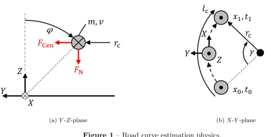
the SAFERIDER1 _{project. The detection strategy is based on the difference between} the actual state of the vehicle and a previewed optimal safe state, which is forecasted with the help of the GPS position. Therefore, a detailed model of the motorcycle’s dynamic behaviour during cornering is essential for real-time applications, see Cossalter et al. [9–11] and Tanelli et al. [12]. The second purpose for estimating the current road curve properties is field data collection, which is part of the main focus of this research. Compared to the detailed and more complex models [9–12], the authors propose a simpler approach, which requires less onboard sensors and is therefore more suitable for field data collection. According to Cossalter [11], a two-wheeled vehicle during cornering can be described as a lumped mass with physical properties mass m, velocity v, and banking angleφ, see Figure1a. During steady-state cornering and on the assumption of infinitely slim tyres and a negligible steering angle, the equilibrium of moments around the X -axis can be applied to obtain the curve radius rc, see Equations (1)–(3). The normal force FN appears due to gravity. The centrifugal force FCen occurs due to the circular movement of the motorcycle around the rotational axis, which is the centre of the curve. The curvatureκ is defined as the inverse of the curve radiusrcand is always positive.

FN=mg, (1) FCen=FNtan|φ|= mv2 rc (2) ⇒rc= v2 gtan|φ|, κ= gtan|φ| v2 . (3)

The developed algorithm detects the beginning of a curve with the help of the absolute value of the banking angle φ. There are two additional conditions. First, the vehicle velocity must exceed a given threshold to omit the detection of banking during parking. Once a curve is detected, the algorithm calculates the running mean of the velocity¯v, the running mean of the banking angleφ¯, and the timespan∆tfor the cornering manoeuvre. When the absolute value of the banking angle falls below a given threshold, the mean curve radiusr¯cand the mean curve angleγ¯are computed, see Figure1band Equation (4). Second, the mean curve angleγ¯must be >60◦ to omit the detection of small curves and

1_{SAFERIDER Consortium is a paradigm of cooperation between the users, the motorcycle industry,}

the ARAS (Advanced rider assistance systems)/OBIS (On bike information systems), subsystems sup-pliers and the Research and Academic world, see www.saferider-eu.org.

φ

𝑚, 𝑣

𝑟

𝐹

𝐹

𝑍

𝑌

𝑋

𝑟

γ

𝑋

𝑌

𝑥

, 𝑡

𝑙

𝑥

, 𝑡

𝑍

Figure 1– Road curve estimation physics.

overtaking manoeuvres. ¯ γ = v¯∆t ¯ rc , ∆t=t1−t0. (4)

For the evaluation of the curve characteristics, preliminary assumptions must be con-sidered. The objective of the algorithm is to classify a curve with feasible parameters. Assuming a curve is designed as a circular arc, it can be described by the curve radius and the curve angle. The obtained parameters mean curve radiusr¯cand mean curve angle ¯γ describe the curve in a geometrical manner, but they lead to a loss of information due to the simplification of the curve as a circular arc. Instead, a road curve is designed with clothoids at the beginning and at the end of the curve to ensure a smooth derivative of the curvatureκ. For this reason, the authors suggest to establish a further parameter named

curviness c, see Figure1band Equation (5). The curvatureκis therefore integrated over the travelled curve path x:

c= lc ∫

0

κ(x)dx with lc=x1−x0. (5)

The calculation of the curviness c requires the length lc of the curve path which can easily be derived from the velocity once the curve is detected. The curviness parameter

curve since the curvature is also defined by κ= ⏐ ⏐ ⏐ ⏐ dγ dx ⏐ ⏐ ⏐ ⏐ . (6)

Although the curviness parameter c has also the dimensions of an angle, it takes the clothoids into account and is more suitable for distorted curves than the pure calculation of the mean curve angle. Therefore, the curvinessc describes the curve by meanings of its curve angle, assuming the curve would have an ideal circular shape with the same overall curvature as the real curve the rider went through. These advantages justify the introduction of the curviness c.

In principle, the obtained parameters describing the curve characteristics can be clas-sified by diverse possibilities, depending on the purpose of classification and memory requirements. The authors prefer a two-dimensional counting of mean curve radius over mean curve angle. This approach allows the identification of challenging curves with a small curve radius and a large curve angle, for example, sharp bends. The number of gradations of the data bins can be chosen by the users. The curviness c can also be classified into bins. To sum up, a single curve can be classified by its mean curve radius ¯

rc, mean curve angleγ¯ and curviness c.

The classification of the curve by its characteristic parameters is a kind of event de-tection and event classification. To score the curviness of a given road or road segment, the travelled distance shall also be considered. Therefore, the authors propose to integ-rate the curvature κ not just over the curve path, but also over a standard distance of

l= 1 km to compute theroad curviness C, see Equation (7).

C =

l

∫

0

κ(x)dx with l= 1 km. (7)

A higher amount of curves as well as the curviness c of the curves located within

l= 1 kmlead to a higher road curvinessC. In contrast to the single event classification, this approach allows a continuous classification of the road segments in terms of curviness. In summary, the curve estimator is based on a lumped-mass model and requires the velocityv and the roll angleφas input signals.

4 Road slope classification

The second part of the road classification system is the evaluation of the travelled eleva-tion gain. Gorges et al. [1] developed a road slope estimator, which estimates the current road slope α (◦) of two-wheeled vehicles with the help of a linear Kalman filter. They utilise the road slope to compute the slope resistance force and finally the wheel forces to identify customer loads. It is also possible to utilise the current road slope for a real-time application, that is, a downhill brake assistant. In the present paper, the road slope is utilised to score the hilliness of a driven road. The difference in altitude is defined as the elevation gain. The knowledge of the elevation gain travelled by the customers helps for a better understanding of the customer usage. In addition, it improves the design of virtual or real measurement campaigns. For a differentiation between positive and negative elevation gain, the road slopeα is prior splitted into only positive and negative values, see Equation (8).

αp= ⎧ ⎨ ⎩ α forα ≥0 0 forα <0 and αn = ⎧ ⎨ ⎩ 0 for α≥0 α for α <0 . (8)

The road slope α is integrated over the distance x to determine the elevation gain h, see Equation (9). hp = ∫ sinαp(x)dx and hn = ∫ sinαn(x)dx. (9) The elevation gain is accumulated separately for positive and negative sign of the road slope in order to compute continuous elevation gains hp and hn for positive and negative values. This distinction makes it possible to differentiate between uphill and downhill ride. The continuous integration of the road slope results in absolute values, which describe the overall amount of elevation gain travelled by the motorcycle. Similar to the road curviness C it is convenient to score the road hilliness H of road segments. Hence, the positive and negative elevation gain for a standard distance of l = 1 km is computed to obtain the road hillinessH, see Equation (10).

Hp = l ∫ 0 sinαp(x)dx and Hn = l ∫ 0 sinαn(x)dx, (10) with l= 1 km.

The road hillinessH is also accumulated separately for positive and negative elevation gain. It can be classified into bins to make an online classification and subsequent count-ing feasible. In contrast to the accumulated values, this approach allows a continuous classification of the road hilliness. In a nutshell, the proposed method takes the velocity

v and the road slopeα as input signals.

5 Road profile estimator

The third part of the road classification system is the road profile estimator. Road roughness causes vehicle vibrations and has a direct influence on vehicle wear, comfort, safety, and fuel consumption. In addition, the dynamic wheel forces induced by road roughness cause road deterioration [13]. For this reason, the knowledge of road roughness has various applications. Road manufacturers and public authorities are interested in the road conditions due to maintenance reasons, see, for example, [14,15]. Moreover, road roughness affects traffic safety and helps defining speed limits. Vehicle engineers utilise the current road roughness for real-time applications, for example, active suspension systems, as shown in [16–21]. The present study aims at the evaluation of the road roughness to derive customer usage profiles in terms of durability, as it is also the focus in [22,23].

Various studies have already been published to estimate the current road profile from mechanical responses of the vehicle, using different techniques. Ngwangwa et al. [15] and Yousefzadeh et al. [24] adopted an Artificial Neuronal Network (ANN) to reconstruct and classify the road profile depending on the measured vehicle responses. One disadvantage of the ANN method is that it requires high computational efforts for an online application and a large set of training data. Imine et al. [25] and Rath et al. [26] developed sliding mode observers to estimate the road profile. Other methods of control theory have been applied by Doumiati et al. [18,19] and Tudón-Martínez et al. [21], who used an adaptive observer with the Q-parameterisation method. The methods of control theory require in general more onboard sensors than the present study can provide. Kalman filters and augmented Kalman filters have been utilised by Doumiati et al. [16], Yu et al. [17], Jeong et al. [27], and Fauriat et al. [23]. Furthermore, anH∞ observer was adopted by

Tudón-Martínez et al. [20]. These methods based on observer theory utilise a Quarter-of-Vehicle model to estimate the road profile. This is unsuitable for motorcycle dynamics, since two-wheeled vehicles have a distinct pitch mode that needs consideration. Burger [22] formulated an inverse control problem to estimate the road profile and solved it with the help of the control-constraints method, which requires the solution of

differential-Lateral road profile

Longitudinal road profiles

𝑋 𝑌

𝑍

Figure 2– Definition of longitudinal road profiles.

algebraic equations. Mathematical optimisation techniques have been applied by Harris et al. [28] and Nordberg [29]. Wavelet transformation of the vehicle’s response signals and a subsequent Adaptive Neuro-Fuzzy Inference System for the road classification has been developed by Qin et al. [30,31]. The application of wavelets has also been accomplished by Solhmirzaei et al. [32]. The rather simple but fast approach of estimating the road profile in the frequency domain with the help of transfer functions has been published by González et al. [14] and Barbosa [33–35].

The cited methods differ in complexity, objective, and computational cost. The present study uses the approach of transfer functions [14,33–35] and extends it to a full-vehicle model with a delayed rear-wheel excitation. The main disadvantage of constant vehicle velocity is eliminated by applying the method just to a small time span with velocity-dependent transfer functions, which is the novel contribution of this research. The ob-jective is to develop an algorithm that can estimate the current road profile continuously with the onboard signals.

5.1 Road profile evaluation

Sayers and Karamihas postulate that “a road profile is a two-dimensional slice of the road surface, taken along an imaginary line” [36]. If the line is following the road direction, the profile is defined to be a longitudinal profile, as illustrated in Figure2. Longitudinal road profiles describe the roughness and texture of the road.

Road profilers evaluate and measure the longitudinal road profile. They exist in several variations. In the 1960’s, the first inertial profilers developed by General Motors Research Laboratories [37] had a breakthrough to measure large road networks at high speed. An accelerometer measures the inertial reference and a non-contacting sensor measures the

relative height, for example, a laser transducer. Inertial profilers must be moving to measure the road roughness and require a minimum speed. They have been proven to produce accurate results even if they cannot collect long road undulations. However, spatial frequencies less than 0.01 cycles/m(wavelengths above 100 m) are negligible for road statistics in sense of durability [36]. Other road profilers have been developed, for instance, the Longitudinal Profile Analyzer [25], whereby a single-wheel trailer is towed by a car and the movement of the wheel is transformed to the profile elevation. A similar road profiler was developed by Barbosa [35], who transformed the wheel movement with the systems transfer function to obtain the road profile. In 1986, the World Bank published the International Road Roughness Experiment [13] to establish a standard for road roughness measurements and evaluation methods. The authors proposed the

International Roughness Index (IRI) to evaluate the road roughness on a single scale. The IRI is a statistical value that is computed with a virtual quarter car travelling over a road profile with a constant velocity of v = 80 km h−1. The accumulated suspension motion y(x) = zs(x)−zu(x) is divided by the travelled distance L, see Equation (11). The sprung mass displacement is defined byzs(x) and the unsprung mass displacement by zu(x). IRI= 1000 1 vL L ∫ 0 |y˙(x)|dx. (11)

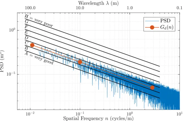
IRI has the unit of slope (m km−1_{). The specific set of parameters characterising the} quarter car system is calledThe Golden Car. The IRI is well known and widely accepted in the automobile industry. One advantage is that it measures the vehicle response to a given road profile and makes a comparison possible. A more detailed description can be found in [13]. Furthermore, ASTM-E1926 [38] defines a standard procedure for computing the IRI. Andrén [39] points out, that the IRI is related to the comfort experienced by a private car, but it is unsuitable for a mathematical description of the road profile. Accordingly, another method to evaluate the road roughness is the power spectral density (PSD) of a road profile. The ISO 8608 [6] defines a method to report the PSD of a given road profile measurement as illustrated in Figure3. The original PSD of an artificial road profile is shown in the spatial frequency domain. According to ISO 8608, the road profile can be classified into eight different road classes (A–H). Furthermore, the ISO proposes a straight line fit Gd(n)with the two parameters roughness coefficient

Gd(n0) and wavinessw, see Equation (12). The roughness coefficient Gd(n0) represents the PSD of the road profile at the reference spatial frequency n0 = 0.1 cycles/m.

Figure 3– PSD and straight line fit of an artificial road profile according to ISO 8608. Gd(n) =Gd(n0) ( n n0 )−w with n0 = 0.1 cycles/m, (12) for 0.011 cycles/m< n <2.83 cycles/m.

The spatial frequency nhas the unitcycles/mand is the inverse of the wavelengthλ. The ISO fixed w = 2, which defines the slope of the fitted PSD. For an evaluation of the straight line fit and other PSD approximations with more parameters, see [39, 40]. For the description of a road profile with a PSD, the road profile is assumed to be a homogeneous and isotropic two-dimensional random process, as Dodds and Robson [41] describe it. On the contrary, Bogsjö [42,43] showed that short segments of irregularities cannot be modelled with Gaussian processes. Hence, Bogsjö et al. [44] proposed a new class of random processes called Laplace models to take the irregularities into account. Furthermore, Johannesson and Rychlik [45] describe a non-stationary Laplace model to stochastically reconstruct the road profile from condensed roughness data in form of IRI. They also formulated a relation between the IRI and the roughness coefficientGd(n0).

Table 1– Properties of the road classes according to ISO 8608 and Sayers and Karamihas [36].

ISO Gd(n0) IRI vmax

Class (10−6_m3_{) (m km}−1_{) Description (m s}−1₎ A 16 1.6 Airport runways and superhighways 60

B 64 3.1 Normal pavements 50

C 256 6.3 Unpaved roads and damaged pavements 30

D 1024 12.5 Rough unpaved roads 20

E 4094 25.1 Enduro tracks 10

F 16 384 49.7 Off-road tracks 5

G 65 536 99.1 Rough off-road tracks 5

H 262 144 198.5 Simulation purpose only 5

5.2 Road profile generation

Synthetic road profiles are required for the development of algorithms to estimate the road roughness. Tyan et al. [46] discussed the two most commonly used methods to create synthetic road profiles: shaping filter and approximation with sinusoids. The first method applies linear digital filters to white noise. This generates coloured noise and in this case pink noise, whose PSD is characterised by a linear declining slope in double logarithmic scale as shown in [30, 47]. The second method is described by Cebon [48] and has been applied by González et al. [14], Ngwangwa et al. [15], and Sun [49]. This method is also utilised by the present research. For the approximation of a pseudo-random road profile zR(x), a large number of N sinusoids with different amplitudes Ai and random phase anglesΦi is superimposed, see Equations (13)–(14).

zR(x) = N ∑ i=1 Aisin (2πnix+ Φi) with (13) Ai = √ Gd(ni)∆n and Φi =U[0,2π). (14)

The amplitudes Ai are calculated from the straight line fit Gd(ni), see Equation (12), for the N different spatial frequencies ni. The relation of the PSD to the amplitude of the road profile is obtained from Fourier analysis, where ∆nis the spatial frequency increment, see Equation (14). The random phase angle Φi is taken from the uniform distribution U. The spatial variable x is defined along the longitudinal direction of the road profile. The reference values Gd(n0) are taken from ISO 8608 [6], which are illustrated in Table1together with an exemplary description of the different road classes [36] and the maximum possible velocity vmax, respectively. Additionally, the IRI is reported for the generated pseudo-random test tracks.

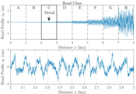
0 1 2 3 4 5 6 7 8 Distancex (km) -1 0 1 R oa d P ro fi le zR (m ) _{A B C} Road Class_{D E F G H} Detail 2 2.1 2.2 2.3 2.4 2.5 2.6 2.7 2.8 2.9 3 Distancex (km) -5 0 5 R oa d P ro fi le zR (c m )

Figure 4– Pseudo random test track comprising road classes A–H and a detailed extract of class C.

classes. For the validation of the developed algorithms, random profiles for all road classes (A–H) were linked together to obtain a complete virtual test track, see Figure4. The upper plot shows the complete test track while the bottom plot shows a detailed extract of the class C road profile. The characteristic PSD of the class C road profile is shown in Figure3. The ISO mentions that road class H is only for simulation purposes. The particular profiles have a length ofl= 1 kmand are multiplied by a window function to ensure a smooth transition between them. This test track enables the development and validation of specific algorithms in order to estimate the current road roughness.

5.3 Full-vehicle model

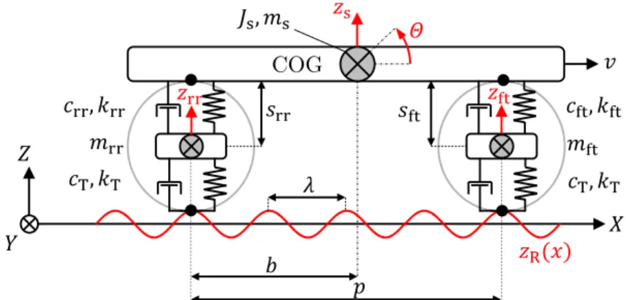
A motorcycle in its plane of symmetry can be represented by three rigid bodies with four independent coordinates. Hence, a full-vehicle model with four degrees of freedom (DOF) was utilised to describe the system dynamics, as illustrated in Figure5. Additionally, the spring deflections are illustrated because they are utilised for the estimation algorithm. The full-vehicle model has been used in several publications to simulate in-plane dynamics of motorcycles, see [11,12, 14, 35, 50]. The in-plane dynamics are generally excited by

𝑝 𝑏 𝑍 𝑋 𝑌 &2* 𝑧R(𝑥) 𝑧_s 𝑧_rr 𝑧ft 𝑚_rr 𝑚_ft 𝜆 𝐽s, 𝑚s _𝛩 𝑣 𝑐ft, 𝑘ft 𝑐_T, 𝑘_T 𝑐_rr, 𝑘_rr 𝑐T, 𝑘T 𝑠_rr 𝑠ft

Figure 5– Full-vehicle model with four DOFs.

road undulationszR(x)and inertial effects due to rider manoeuvres such as accelerating and braking. On the assumption of a constant vehicle velocity v, the in-plane dynamics are reduced to four DOFs: vertical motion of the chassis zs, pitch of the chassis Θ, rear unsprung mass motion zrr, and front unsprung mass motionzft. These four DOFs are related to the vibration modes: bounce, pitch, front wheel hop, and rear wheel hop [12]. The sprung mass ms has the moment of inertia Js and comprises the frame, the engine, the chassis, and the rider. Additionally, parts of the front and rear suspension system are counted to the sprung mass. The sprung mass is lumped in the centre of gravity (COG). The rear unsprung massmrrcomprises the rear wheel, the rear brake, and parts of the rear suspension. The front unsprung massmftcomprises the front wheel, the front brake, and parts of the front suspension. Furthermore, the main geometric dimensions are illustrated: wheelbasepand perpendicular distancebof the COG from the rear-wheel

Z-axis. The lumped masses are connected with parallel spring-damper elements, which are represented by reduced stiffness and damping coefficients for front suspension (kft, cft) and rear suspension (krr, crr). The tyre stiffness and damping coefficients are defined by

kTandcT. The full-vehicle model properties used for this study are illustrated in Table2. The reduced stiffness and damping coefficients are derived with the help of a multi-body simulation. The equations of motion of the full-vehicle model with road excitation are as follows:

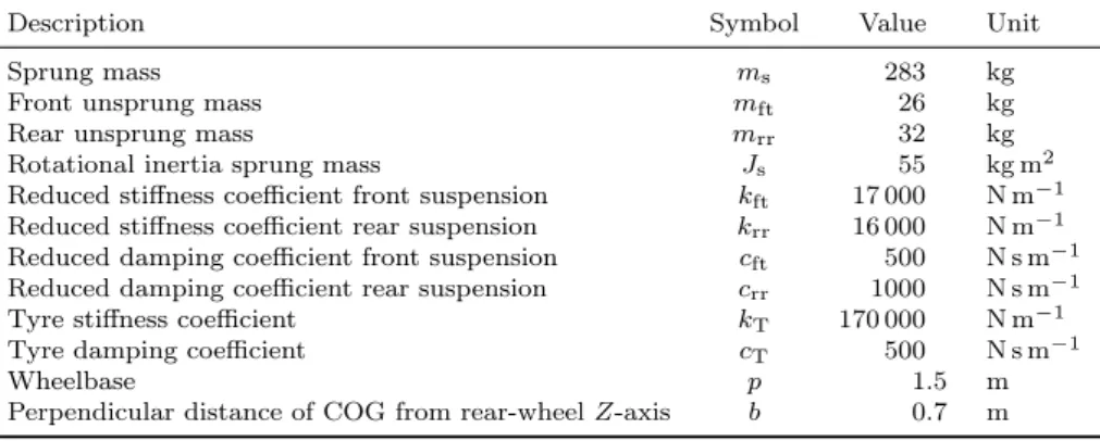
Table 2– Full-vehicle model properties.

Description Symbol Value Unit

Sprung mass ms 283 kg

Front unsprung mass mft 26 kg

Rear unsprung mass mrr 32 kg

Rotational inertia sprung mass Js 55 kg m2 Reduced stiffness coefficient front suspension kft 17 000 N m−1 Reduced stiffness coefficient rear suspension krr 16 000 N m−1 Reduced damping coefficient front suspension cft 500 N s m−1 Reduced damping coefficient rear suspension crr 1000 N s m−1 Tyre stiffness coefficient kT 170 000 N m−1 Tyre damping coefficient cT 500 N s m−1

Wheelbase p 1.5 m

Perpendicular distance of COG from rear-wheelZ-axis b 0.7 m

Mx¨+Cx˙ +Kx=F with (15) x= ⎛ ⎜ ⎜ ⎜ ⎜ ⎝ zs Θ zft zrr ⎞ ⎟ ⎟ ⎟ ⎟ ⎠ , M= ⎡ ⎢ ⎢ ⎢ ⎢ ⎣ ms 0 0 0 0 Js 0 0 0 0 mft 0 0 0 0 mrr ⎤ ⎥ ⎥ ⎥ ⎥ ⎦ , (16) C= ⎡ ⎢ ⎢ ⎢ ⎢ ⎣ cft+crr cft(p−b)−crrb −cft −crr cft(p−b)−crrb cft(p−b)2+crrb2 −cft(p−b) crrb −cft −cft(p−b) cft+cT 0 −crr crrb 0 crr+cT ⎤ ⎥ ⎥ ⎥ ⎥ ⎦ , (17) K= ⎡ ⎢ ⎢ ⎢ ⎢ ⎣ kft+krr kft(p−b)−krrb −kft −krr kft(p−b)−krrb kft(p−b)2+krrb2 −kft(p−b) krrb −kft −kft(p−b) kft+kT 0 −krr krrb 0 krr+kT ⎤ ⎥ ⎥ ⎥ ⎥ ⎦ , (18) F = ⎛ ⎜ ⎜ ⎜ ⎜ ⎝ 0 0 kTzR(t) +cTz˙R(t) kTzR(t−τ) +cTz˙R(t−τ) ⎞ ⎟ ⎟ ⎟ ⎟ ⎠ . (19)

On the assumption that the rear wheel follows the same road profile as the front wheel, the road excitation of the rear wheel is the same function as for the front wheel with a time delayτ:

τ = p

This implies that the excitation of the system depends on the vehicle velocity v. Moreover, this formulation makes a single-input multiple-output (SIMO) system defini-tion possible to analyse the dynamic behaviour of the system as a funcdefini-tion of the road roughnesszR(t). Linear time-invariant (LTI) systems are suitable to analyse the response of a system to an arbitrary input in the time and frequency domain. The aforementioned full-vehicle model is therefore formulated as an LTI system, since the matrices are linear and the solution is linear shift-invariant. The relation between the excitation and the response of the system is described with transfer functionsH(s), which relate the output

Y(s) to the inputX(s) in the frequency domain:

H(s) = Y(s)

X(s) =

L{y(t)}

L{x(t)}. (21)

The Laplace transformation of the system equations needs to be derived to obtain the transfer functions. For the formulation with just one input variable for the road roughness ZR(s), the shift theorem as well as the derivation theorem from the Laplace transformation rules are used as follows:

L{zR(t)}=ZR(s), (22) L{zR(t−τ)}=ZR(s)e−τ s, (23) L{z˙R(t)}=sZR(s), (24) L{z˙R(t−τ)}=sZR(s)e−τ s. (25) The Laplace transformation of the system equations assuming zero initial conditions is given by: s2MX(s) +sCX(s) +KX(s) = ⎛ ⎜ ⎜ ⎜ ⎜ ⎝ 0 0 kTZR(s) +scTZR(s) kTZR(s)e−τ s+scTZR(s)e−τ s ⎞ ⎟ ⎟ ⎟ ⎟ ⎠ . (26)

X(s) is the Laplace transformation of the input x(t). The equations of the spring deflections sft, srr are derived and subsequently transformed to the frequency domain, see Equations (27)–(28).

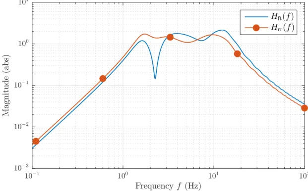
10−1 ₁₀0 ₁₀1 ₁₀2 Frequencyf (Hz) 10−3 10−2 10−1 100 101 M ag n it u d e (a b s) H_ft(f) H_rr(f)

Figure 6– Bodeplot of transfer functions forv= 15 m s−1.

Sft(s) =Zs(s) + (p−b)Θ(s)−Zft(s), (27)

Srr(s) =Zs(s)−bΘ(s)−Zrr(s). (28)

The onboard signals comprise the front spring deflectionsftand the rear spring deflec-tionsrr. For this reason, the following two transfer functions are formulated:

Hft(s, v) = Sft(s)

ZR(s)

, Hrr(s, v) = Srr(s)

ZR(s)

. (29)

The input variable is the road roughness ZR(s), respectively. The transfer functions can be derived by solving Equations (26)–(28) numerically. Since the road roughness excites the rear wheel depending on the time delayτ, the transfer functions are functions of the vehicle velocity v. Figure 6 shows the magnitude part of the bode plot of the two transfer functions for a vehicle velocity of v = 15 m s−1. These transfer functions describe the frequency response of the respective output signals to the road excitation. In the following, they are used to estimate the road profile with the onboard signals.

5.4 Estimation algorithm

The relation between the response and the road profile in the time frequency domain

f can be expressed with transfer functions, as shown in Equation (29). To apply the transfer functions to the PSD signals, the magnitude part of the transfer function needs to be squared. This relates the PSD of the response signal PSDRes(f)to the PSD of the road profile PSD_Road(f), as shown in Equation (30).

|H(f)|2= PSDRes(f)

PSDRoad(f) ⇒ PSDRoad(f) =

PSDRes(f)

|H(f)|2 . (30) This means that the PSD of the road profile can be determined with the PSD of the response signal and the associated transfer function. The PSD must be transformed to the spatial frequency domain nto determine the road class according to ISO 8608 with the following relation:

n= f

v and PSDRoad(n) =vPSDRoad(f). (31)

The formulation PSD_Road(n) = vPSD_Road(f) follows from the definition of the PSD as the squared amplitude per frequency increment. In summary, the characteristic PSD of the road profile can be determined with the following expression:

PSD_Road(n) = vPSDRes(f)

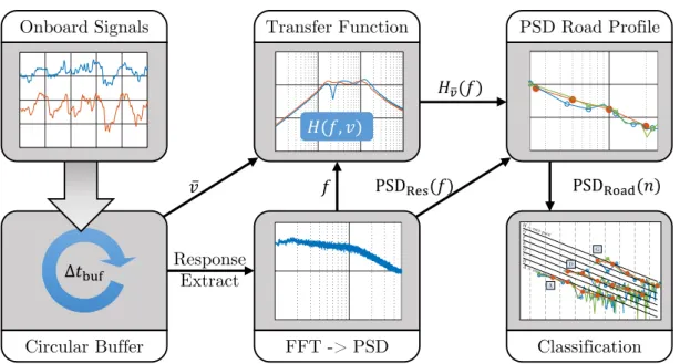
|H(f)|2 . (32) This approach is based on the assumption of a constant velocity v. For the develop-ment of a method that is feasible to estimate the current road roughness under realistic operating conditions, the algorithm must be fast and independent of a constant vehicle velocity. Hence, the approach is modified as follows: The transfer functions are calcu-lated in advance for a range of different velocities. As a result, the function stackH(f, v) provides the correct transfer functionHv(f) depending on the velocity. For a continuous estimation of the PSD of the road profile, an algorithm was developed, as illustrated in Figure 7. Starting from the onboard signals, a circular ring buffer records the required signals for a given time span ∆tbuf. Subsequently, the mean value of the velocity v¯ is calculated for the extracted time frame. In the meantime, the fast Fourier transform (FFT) and PSD of the signal PSDRes(f)are computed in the time domain. The correct transfer function is interpolated from the transfer function stack for the given mean ve-locity v¯ and the calculated frequenciesf resulting from the FFT. Afterwards, the PSD of the road profile PSDRoad(n)can be calculated according to Equation (32), followed by the classification algorithm. The choice of the time span ∆tbuf has an influence on the

Transfer Function

Onboard Signals PSD Road Profile

FFT -> PSD Classification Circular Buffer

Δ𝑡_buf Response_Extract

𝑣 𝑓 PSD_Res(𝑓)

𝐻 _𝑣(𝑓)

PSDRoad(𝑛)

𝐻(𝑓, 𝑣) 𝐻(𝑓, 𝑣)

Figure 7– Flow chart of the road profile estimation algorithm.

classification quality and is evaluated in Section6.3.

5.5 Road profile classification

As introduced in Section5.1, the PSD of the road profile can be evaluated by ISO 8608 [6]. According to this standard, the PSD of the road profile can be classified either at the spatial reference frequencyn0 = 0.1 cycles/mor multiple times in every single octave band. The first method has the disadvantage that the classification result depends only on the PSD value at the spatial reference frequency. Furthermore, it assumes that a straight-line fit can approximate the PSD. As Andrén [39] showed, PSDs from real road measurements deviate from this assumption. The classification in every single octave band is also infeasible for the present research, since different classification results in the single octave bands must be stored for every time segment. Moreover, this method gives indistinct classification results. Hence, the main objective is the classification of a road segment by its PSD into a single category with the maximum of information provided.

For this reason, the authors propose a novel method to classify the PSD of a road profile for a given time- or distance segment. After the PSD of the road profile has been calculated according to Equation (32), it is smoothed in 10 octave bands, which are illustrated in Table3 and which are proposed by ISO 8608 [6]. The centre frequency in each octave band is calculated by nc = 2EXP. The authors propose the following novel smoothing algorithm. Weighted average values of the PSD in the respective octave bands

Table 3– Octave bands and geometric mean values for road classification.

Geometric mean values for road classes according to ISO 8608

nc Gd(nc)(10−6m3) EXP (cycles/m) A B C D E F G H −7 0.007 86 2621 10 486 41 943 167 772 671 089 2 684 354 10 737 417 42 949 668 −6 0.0156 655 2621 10 486 41 943 167 772 671 089 2 684 354 10 737 417 −5 0.0313 164 655 2621 10 486 41 943 167 772 671 089 2 684 354 −4 0.0625 41 164 655 2621 10 486 41 943 167 772 671 089 −3 0.125 10 41 164 655 2621 10 486 41 943 167 772 −2 0.25 2.56 10 41 164 655 2621 10 486 41 943 −1 0.5 0.64 2.56 10 41 164 655 2621 10 486 0 1 0.16 0.64 2.56 10 41 164 655 2621 1 2 0.04 0.16 0.64 2.56 10 41 164 655 2 4 0.01 0.04 0.16 0.64 2.56 10 41 164

are calculated to smooth the PSD. The weighted average is performed by a normalised Gaussian window function for each octave band. This smoothing algorithm ensures a correct value of the PSD at the respective centre frequency nc, even if only a few values are available within each octave band. This is necessary since different velocities result in different spatial frequency at which the PSD is calculated. In addition, the smoothing in octave bands provides a uniform distribution of PSD values over the spatial frequencies. This is also necessary because the classification is treated in the logarithmic domain. The output of the smoothing algorithm is PSD_Smoothed(nc). At this point, the algorithm can handle multiple estimates of the road profile from different onboard sensors. Subsequently, one smoothed spectrum is calculated.

The classifier is formulated as a minimum distance classifier, which calculates the distances of PSDSmoothed(nc)from the geometric mean values of the different road classes in every single octave band. The matrix M(nc,class) of geometric mean values of the different road classes in the respective octave bands is illustrated in Table 3. The road profile is classified as the road class with the minimum sum of distances, according to Equation (33).

Road class= min {₁₀

∑

i=1

|log₁₀[PSD_Smoothed(nc,i)]−log10[M(nc,i,class)]| }

. (33)

Figure 8 illustrates three different examples of road profile classification for different segments. The classified road classes are denoted beside the graphs. At first, the original PSDs of the road profile estimation algorithm are smoothed in the specified octave bands, which are highlighted with dashed lines. For these examples, the front and rear spring deflection signals have been used to estimate the road profile. It can be seen that the

Figure 8– Examples of road profile classification.

smoothed PSD is the mean of the two provided PSD estimates PSD_ft(n) and PSD_rr(n). Finally, the minimum sum of distances classifies each road segment. The PSDs are located at different spatial frequencies, which is a result of different velocities at each segment. For example, road segment categorised to class A was driven at a velocity of

vA = 60 m s−1. Road segment class D was driven at a velocity of vD= 15 m s−1. Road segment class G was driven at a velocity of vG = 5 m s−1. Further influences on the frequencies resulting from the FFT are the time span ∆tbuf and the sample frequency, which is set tof = 100 Hz.

One advantage of this classification method is its modular approach. The more onboard sensors are available, the more robust becomes the classification result. The smoothing algorithm can easily be extended to calculate the mean values of more than just one PSD estimation. Additional transfer functions can be derived from the full-vehicle model depending on the available onboard sensors. After the road class has been determined, the travelled distance can be calculated from the mean velocity. The distances in the road classes are incremented by the respective segment distance. Thus, a distribution of travelled road classes can be recorded for the customer usage profiles.

800 900 1000 1100 1200 1300 1400 1500

X

(m)

Y

(m

)

Curviness

c

(rad)

14

13

12

11

10

9

8

7

6

5

4

3

2

1

Figure 9– Results of the road curve estimator.

6 Results and Validation

6.1 Validation of the road curve estimator

A test ride with the reference motorcycle as described in Section 2 was performed on a curvy road to validate the road curve estimator. Figure 9 shows an extract of the driven test road and the classified curves, respectively. The coloured sections highlight the identification of a curve while the colour itself represents the curviness c of the classified curves. It can be seen for example that curve No. 11 has the highest curviness score, while curve No. 9 has the lowest curviness score. All curves were identified by the curve estimator, which indicates the robustness of the developed algorithm. The particular curve properties mean curve radius r¯c, mean curve angle ¯γ, and curviness

c are illustrated in Table 4. It can also be seen that the distorted curve No. 11 was scored with a high curviness even if the mean curve angle ¯γ was scored not that high

Table 4– Properties of the classified road curves.

Road curve No.

Property 1 2 3 4 5 6 7 8 9 10 11 12 13 14 ¯ rc(m) 43 49 35 98 38 77 35 42 70 35 61 33 28 30 ¯ γ(◦) 113 85 254 119 218 103 208 78 74 112 182 184 237 130 c(rad)×10−2 _{169 123 388 226 358 181 319 117 114 166 408 319 396 207} 1060 1080 1100 1120 1140 1160

X

(m)

Y

(m

)

¯

r

= 35m

¯

γ

= 208

c

= 3

.

19rad

GPS

Curve Detection

Classi

_fi

cation Result

Figure 10– Properties of road curve No. 7.

in comparison to the other curves. This manifests the proposed index curviness c as an curve-evaluation index.

Figure 10 shows the classification results of curve No. 7 in more detail. The curve estimator detected the correct beginning and end of the curvature of the road, which is represented by the solid line (Curve Detection). In addition, the estimated curve properties are highlighted with a circular arc with geometric dimensions according to the estimation results (Classification Result). It can be seen that the estimated circular arc roughly fits to the real road curvature. The overestimation is a result of the curve construction with clothoids, as can be seen at the beginning and end of the curve in Figure 10. These parts also contribute to the estimation algorithm. The calculation of the running mean of the roll angle results in curve properties that are a compromise between the smallest curve radius and the clothoids of the curve. The proposed method is well suited to detect and classify curves in order to collect customer usage profiles and to evaluate the driven curves. In addition, the road curvinessC continuously scores

0 0.2 0.4 0.6 0.8 1 1.2 1.4 1.6 1.8 2

X

_(km)

Y

(k

m

)

Road Curviness

C

_(rad)

5

4

3

2

1

Figure 11– Results of the road curviness classification.

road segments of l = 1 km, as illustrated in Figure 11. It can be seen that the road curviness scores the respective road segment depending on the amount and curviness of curves within the segment. The road curviness C was scored to 9,11,15, 17, and 6 (rounded) for the given road segments No. 1–5. Road segment No. 4 was scored with the highest road curviness C. This is reasonable due to the amount of sharp curves within the segment. In contrast to the single curve classification, the continuous classification of road segments makes a characterisation of the driven roads possible.

The lumped-mass model achieved sufficient results for the scope of customer usage profiles. The classified curve properties can be counted online, whereas the number of gradations is chosen by the user and the memory capacities. Since the algorithm is based on the response of the vehicle, the estimated curve properties are based on the driving line of the motorcycle. Thus, different curve driving techniques can lead to different results for the same curve. The differences are assumed to be negligible in terms of customer usage profiles.

6.2 Road slope classification

The road slope estimator developed by Gorges et al. was validated with the help of a mountain road in a previous publication [1]. In the present paper, this mountain road has been utilised to show the results of the road slope classification method. The mountain road was driven uphill and downhill with the reference motorcycle, as shown in the upper plot of Figure12. The counting results of the road hilliness H are illustrated in the bottom plot for positive and negative values, respectively. The road hilliness

600 700 800 900

A

lt

it

u

d

e

(m

)

Distance (km)

H

(m

/k

m

)

H

_H

Figure 12– Results of the road slope classification.

H counts the positive and negative elevation gain per kilometre. The overall elevation gain for this ride was counted to hp = 342 m and hn = −343 m. Once the road slope estimator is implemented in the vehicle, it is convenient to count the elevation gain with the presented method. The distribution of an overall elevation gain as part of the customer usage profiles is favourable for the vehicle development process, since it affects vehicle design targets and improves the understanding of the customer behaviour. The travelled elevation gain has a direct influence on the powertrain design and on the brake design. In addition, the classification of the particular road segments improves the choice of real test road or for the design of virtual test tracks.

6.3 Validation of the road profile estimator

Real roads are not characterised by a homogeneous road class, as highlighted by Andrén [39] and Bogsjö [42, 43]. Furthermore, arbitrary roads are in general not surveyed by a road profiler, which makes a validation infeasible. For this reasons, the validation of the road profile estimator was achieved by numerical simulation, for which the full-vehicle model was excited by the pseudo-random test track as presented in Section 5.2. The simulation was performed by the ode45-solver of MATLAB⃝R, which is based on

the Runge–Kutta method. Each of the eight road class segments (A–H) was travelled with a constant acceleration of the motorcycle. This guarantees that the estimator was tested under variable velocities and that all possible frequencies in the range of use have been excited. The maximum velocities vmax for the respective road classes were chosen with respect to the physical limitations of a motorcycle travelling over the tracks. The minimum velocity isvmin= 3 m s−1, which is the minimum required velocity for the road profile estimator. Each road class was driven for a time period of t = 100 s. Since the full-vehicle model has no degree of freedom in the longitudinal direction, the variable velocity was realised through the transformation of the road profile from the spatial domain to the time domain. Figure 13 shows the results of the simulation. The upper plot shows the linear slope of the velocityvin every road class segment together with the maximum velocities vmax, respectively. The last three road classes (F–G) were driven with a maximum velocity ofvmax= 5 m s−1 because they represent heavy off-road tracks which are difficult to ride even for an enduro motorcycle like the reference vehicle. The middle plot shows the respective road profile zR(t). It gets rougher with an increase in the road class. The bottom plot shows the classification results of the road profile estimator. It can be seen that almost all predicted road classes are classified correctly. The time span was set to ∆tbuf = 1 s. This means that 100 time segments have been classified per road class. A total of four estimates have been classified false, but only by a one road-class difference. This indicates that the proposed method is robust and highly accurate. As is common in classification analysis, the results are reported in a confusion matrix, see Table5.

The entries contain the amount of respective classifications. The last row and column illustrate the percentage of correct classified values in each class. An overall classification result of 99.5 % was achieved. A higher time span∆tbuf leads to a more robust result, since the signal length and thus the frequency content gets higher. On the other hand, under the assumption of a variable velocity, the transfer function gets ambiguous and therefore the classification quality gets worse. Additionally, the road quality can change very fast, so that a longer time period results in an indistinct classification result. In the end, the choice of the time span ∆tbuf is a compromise between reaction speed and quality. The underlying method of the PSD calculation has also an influence on the classification result. Since the smoothing algorithm is applied after the PSD calculation, an overlapped PSD calculation method is not necessary to achieve a robust result. In addition, this would lead to a loss of frequency resolution, which is essential for the road classification algorithm.

0 10 20 30 50 60

V

el

o

ci

ty

v

(m

/s

)

_A

_B

_C

Actual Class

_D

_E

_F

_G

_H

z

(m

)

Time

t

(s)

P

re

d

ic

te

d

C

la

ss

Figure 13– Validation of the road profile estimator.

Table 5– Confusion matrix of the road profile estimator.

Actual class A B C D E F G H ∑ (%) Predicted class A 100 0 0 0 0 0 0 0 100 B 0 100 0 0 0 0 0 0 100 C 0 0 100 0 0 0 0 0 100 D 0 0 0 100 0 0 0 0 100 E 0 0 0 0 100 1 0 0 99 F 0 0 0 0 0 98 1 0 99 G 0 0 0 0 0 1 99 1 98 H 0 0 0 0 0 0 0 99 100 ∑ (%) 100 100 100 100 100 98 99 99 99.5

under variable velocity, which had been addressed as a disadvantage of this method in the past [20,21,23]. The reaction time is fast enough for collecting customer usage profiles and implementing it into real-time control systems. Furthermore, the modular approach makes the presented method easily extensible depending on the available onboard sensors. In addition, the computational effort is less compared to the alternative methods. An online application is therefore feasible. The developed road profile estimator requires a full-vehicle model of the motorcycle, the velocityv, and at least one suspension deflection signal as input. The derivation of transfer functions requires an LTI system formulation. Thus, the model has to be reduced to a linear system.

7 Summary and Conclusion

The objective of this research was to develop a road classification system with onboard signals of two-wheeled vehicles. First, a curve estimation algorithm was developed, which identifies and classifies curves on the driven road. The authors propose a method to evaluate every single curve by its mean curve radius, mean curve angle, and its curviness – a quantity that expresses how intense a rider would experience the curve. The algorithm takes the velocity and the roll angle as input signals. Beside the event detection, the road curviness continuously evaluates the underlying road to gather information about the driven road segments. The results show that the curve estimator works as expected and that curves are classified in accordance with their geometric dimensions. Second, the road slope was utilised to classify the hilliness of the driven road. An absolute value of the elevation gain can be obtained through the continuous integration of the road slope over the distance travelled. The road hilliness continuously evaluates the elevation gain per road segment. The proposed method takes the velocity and the road slope as input signals.

Third, a road profile estimator was developed. Different evaluation methods are presen-ted for a scientific classification of the road profile. The authors decided to utilise a frequency approach, which is fast and easy to implement, but was supposed to have some disadvantages in the past. The transfer functions of a two-wheeled vehicle were derived with the help of a full-vehicle model and the Laplace transformation. In con-trast to previous publications which utilised a simple quarter-car model, the presented model excites the front and rear wheel and is formulated with just one input variable, the road roughness. This enables the correct application of the transfer functions, which describe the relationship between the suspension deflections and the road profile. The presented estimation algorithm is formulated in the frequency domain and does not rely

on a constant velocity assumption, which was addressed as a disadvantage so far. The results show that the classification algorithm detects the correct road class within one second. The road profile estimator is highly accurate and robust. The modular approach makes it easily adaptable and extendable to the available onboard signals. The classi-fication algorithm is based on the ISO 8608 standard. It has successfully been proven on a virtual test track. It has to be mentioned that the transfer functions as well as the validation have been achieved by the same numerical model of the full vehicle model. For this reason, the results are quite good. The proposed method will be verified with a real motorcycle on existing roads in further research. The nonlinear behaviour of the tyres, the spring-damper system and the influence of the vehicle dynamics needs to be investigated. The road profile estimator works fast and requires no excessive computa-tional effort compared to other methods. The presented method requires a linearised full-vehicle model of the motorcycle, the velocity, and at least one suspension deflection signal as inputs.

All of the developed algorithms are feasible to work in real time. For this reason, an implementation into existing electronic control units is feasible. Vehicle design targets can incrementally be improved with the knowledge of the road class distribution. It helps understanding the customer usage and it enables to develop further customer-specific applications. Another benefit is the evaluation of measurement campaigns compared to the customer profiles. In addition, the distribution of different road classes makes a virtual load acquisition possible, where a virtual vehicle collects load data on a virtual test track. The vehicle-independent road classification enables a comparison between different product segments and different markets. In the future, detailed knowledge about customer usage profiles offers a variety of applications throughout the automotive business.

Since no time and location stamps are collected, an implementation of the system is assumed to be uncritical in terms of data privacy. The data is collected anonymously without any customer assignment. The resultant customer distribution is treated statist-ically to derive values such as quantiles, which do not correspond to individual customers. Further research is planned to validate the developed road profile estimator on real roads of different road classes. In addition, the detection and classification of irregularities, that is, potholes, within the road segments will be analysed.

References

[1] C. Gorges, K. Öztürk and R. Liebich. ‘Customer loads of two-wheeled vehicles’. In:

[2] P. Johannesson and M. Speckert, eds.Guide to load analysis for durability in vehicle engineering. Chichester: Wiley, 2013, p. 434.

[3] L. Müller. ‘Mehrkörpermodell-basiertes Online Monitoring der Betriebsbeanspruchung am Beispiel eines Nutzfahrzeug-Demonstrators’. PhD thesis. Kaiserslautern: TU Kaiserslautern, 2011.

[4] C. Matz. ‘Online Berechnung von Fahrwerkskräften auf Basis von Onboard-Sensorik’. PhD thesis. Clausthal: TU Clausthal, 2015.

[5] M. Karlsson. ‘Load modelling for fatigue assessment of vehicles – a statistical ap-proach’. PhD thesis. Göteborg, Sweden: Chalmers, Göteborg University, 2007. [6] ISO. Mechanical vibration - Road surface profiles - Reporting of measured data.

Standard No. 8608:2016. Geneva, Switzerland: ISO, 2016.

[7] M. Speckert, K. Dressler, N. Ruf et al. ‘The virtual measurement campaign (VMC) concept’. In:Commercial Vehicle Technology 2014. Kaiserslautern, Germany: Shaker Verlag, Mar. 2014, pp. 88–98.

[8] F. Biral, M. Da Lio, R. Lot et al. ‘An intelligent curve warning system for powered two wheel vehicles’. In:Eur. Transp. Res. Rev.2.3 (2010), pp. 147–156.

[9] V. Cossalter, A. Doria and R. Lot. ‘Steady turning of two-wheeled vehicles’. In:

Vehicle System Dynamics 31.3 (1999), pp. 157–181.

[10] V. Cossalter and R. Lot. ‘A motorcycle multi-body model for real time simulations based on the natural coordinates approach’. In: Vehicle System Dynamics 37.6 (2002), pp. 423–447.

[11] V. Cossalter.Motorcycle Dynamics. 2nd ed. [place unknown]: LULU, 2006, p. 372. [12] M. Tanelli, M. Corno and S. M. Savaresi, eds.Modelling, simulation and control of

two-wheeled vehicles. Chichester: Wiley, 2014, pp. 1–348.

[13] M. W. Sayers, T. D. Gillespie and C. A. V. Queiroz.The international road rough-ness experiment. Washington, D.C.: The World Bank, 1986.

[14] A. González, E. J. O’brien, Y.-Y. Li et al. ‘The use of vehicle acceleration meas-urements to estimate road roughness’. In: Vehicle System Dynamics 46.6 (2008), pp. 483–499.

[15] H. M. Ngwangwa, P. S. Heyns, F. J. J. Labuschagne et al. ‘Reconstruction of road defects and road roughness classification using vehicle responses with artificial neural networks simulation’. In:J. Terramechanics 47.2 (2010), pp. 97–111. [16] M. Doumiati, A. Victorino, A. Charara et al. ‘Estimation of road profile for vehicle

dynamics motion: experimental validation’. In:American Control Conference. San Francisco: IEEE, June 2011, pp. 5237–5242.

[17] W. Yu, X. Zhang, K. Guo et al. ‘Adaptive real-time estimation on road disturbances properties considering load variation via vehicle vertical dynamics’. In:Math. Probl. Eng.2013 (2013), pp. 1–9.

[18] M. Doumiati, S. Erhart, J. Martinez et al. ‘Adaptive control scheme for road profile estimation: application to vehicle dynamics’. In: The International Federation of Automatic Control. Cape Town: IFAC, Aug. 2014, pp. 8445–8450.

[19] M. Doumiati et al. ‘Road profile estimation using an adaptive Youla–Kučera para-metric observer: Comparison to real profilers’. In: Control Engineering Practice

61.2002 (Apr. 2017), pp. 270–278.

[20] J. C. Tudón-Martínez, S. Fergani, O. Sename et al. ‘Online road profile estimation in automotive vehicles’. In:European Control Conference (ECC). Strasbourg: ECC, June 2014, pp. 2370–2375.

[21] J. C. Tudón-Martínez, S. Fergani, O. Sename et al. ‘Adaptive road profile estim-ation in semiactive car suspensions’. In: IEEE Transactions on Control Systems Technology 23.6 (2015), pp. 2293–2305.

[22] M. Burger. ‘Calculating road input data for vehicle simulation’. In:Multibody Syst. Dyn.31.1 (2013), pp. 93–110.

[23] W. Fauriat, C. Mattrand, N. Gayton et al. ‘Estimation of road profile variabil-ity from measured vehicle responses’. In: Vehicle System Dynamics 54.5 (2016), pp. 585–605.

[24] M. Yousefzadeh, S. Azadi and A. Soltani. ‘Road profile estimation using neural network algorithm’. In:Journal of Mechanical Science and Technology 24.3 (2010), pp. 743–754.

[25] H. Imine, Y. Delanne and N. K. M’Sirdi. ‘Road profile input estimation in vehicle dynamics simulation’. In:Vehicle System Dynamics 44.4 (2006), pp. 285–303. [26] J. J. Rath, K. C. Veluvolu and M. Defoort. ‘Simultaneous estimation of road profile

and tire road friction for automotive vehicle’. In:IEEE Transactions on Vehicular Technology 64.10 (2015), pp. 4461–4471.

[27] W. Jeong, K. Yoshida, H. Kobayashi et al. ‘State estimation of road surface and vehicle system using a Kalman filter’. In:JSME Int. J. 33.4 (1990), pp. 528–534. [28] N. K. Harris, A. González, E. J. O’Brien et al. ‘Characterisation of pavement profile

heights using accelerometer readings and a combinatorial optimisation technique’. In:Journal of Sound and Vibration 329.5 (2010), pp. 497–508.

[29] T. P. Nordberg. ‘An iterative approach to road/profile identification utilizing wave-let parameterization’. In:Vehicle System Dynamics 42.6 (2004), pp. 413–432. [30] Y. Qin, M. Dong, F. Zhao et al. ‘Road profile classification for vehicle semi-active

suspension system based on adaptive neuro-fuzzy inference system’. In:Conference on Decision and Control (CDC). Osaka: IEEE, Dec. 2015, pp. 1533–1538.

[31] Y. Qin, M. Dong, R. Langari et al. ‘Adaptive hybrid control of vehicle semiactive suspension based on road profile estimation’. In:Shock Vib. 2015.1 (2015), pp. 1– 13.

[32] A. Solhmirzaei, S. Azadi and R. Kazemi. ‘Road profile estimation using wavelet neural network and 7-DOF vehicle dynamic systems’. In: Journal of Mechanical Science and Technology 26.10 (2012), pp. 3029–3036.

[33] R. S. Barbosa. ‘Vehicle dynamic response due to pavement roughness’. In: J. Brazilian Soc. Mech. Sci. Eng.XXXIII.3 (2011), pp. 302–307.

[34] R. S. Barbosa. ‘Vehicle dynamic safety in measured rough pavement’. In:Journal of Transportation Engineering 137.5 (2011), pp. 305–310.

[35] R. S. Barbosa. ‘Vehicle vibration response subjected to longwave measured pave-ment irregularity’. In:J. Mech. Eng. Autom.2.2 (2012), pp. 17–24.

[36] M. W. Sayers and S. M. Karamihas.The little book of profiling. Michigan: University of Michigan, 1998.

[37] E. B. Spangler and W. J. Kelly.GMR road profilometer: a method for measuring road profile. Tech. rep. GMR-452. Warren, Michigan: General Motors Corporation Research Laboratories, 1964.

[38] ASTM International. Standard practice for computing international roughness in-dex of roads from longitudinal profile measurements. Standard No. E1926-08. West Conshohocken (PA): ASTM International, 1999.

[39] P. Andrén. ‘Power spectral density approximations of longitudinal road profiles’. In:International Journal of Vehicle Design 40.1/2/3 (2006), pp. 2–14.

[40] B. R. Davis and A. G. Thompson. ‘Power spectral density of road profiles’. In:

Vehicle System Dynamics 35.6 (2001), pp. 409–415.

[41] C. J. Dodds and J. D. Robson. ‘The description of road surface roughness’. In:

Journal of Sound and Vibration 31.2 (1973), pp. 175–183.

[42] K. Bogsjö. ‘Development of analysis tools and stochastic models of road profiles regarding their influence on heavy vehicle fatigue’. In: Vehicle System Dynamics

44.sup1 (2006), pp. 780–790.

[43] K. Bogsjö. ‘Road profile statistics relevant for vehicle fatigue’. PhD thesis. Lund, Sweden: Lund University, 2007.

[44] K. Bogsjö, K. Podgórski and I. Rychlik. ‘Models for road surface roughness’. In:

Vehicle System Dynamics 50.5 (2012), pp. 725–747.

[45] P. Johannesson and I. Rychlik. ‘Modelling of road profiles using roughness indic-ators’. In:International Journal of Vehicle Design 66.4 (2014), p. 317.

[46] F. Tyan, Y.-F. Hong, S.-H. Tu et al. ‘Generation of random road profiles’. In:J. Adv. Eng.4.2 (2009), pp. 151–156.

[47] F. Schube. ‘Beitrag zur numerischen Simulation des Wirbelsäulenverhaltens eines Kraftfahrers infolge durch Straßenunebenheiten induzierter Ganzkörperschwingun-gen’. PhD thesis. Aachen, Germany: RWTH Aachen, 2002.

[48] D. Cebon. Handbook of vehicle-road interaction. Advances in engineering. Boca Raton, Florida: CRC Press, 2000.

[49] L. Sun. ‘Simulation of pavement roughness and IRI based on power spectral dens-ity’. In:Math. Comput. Simul.61.2 (2003), pp. 77–88.

[50] V. Cossalter et al. ‘Frequency-domain method for evaluating the ride comfort of a motorcycle’. In:Vehicle System Dynamics 44.4 (2006), pp. 339–355.