Lagrangian Support Vector Machines
O. L. Mangasarian
David R. Musicant
Computer Sciences Dept. Dept. of Mathematics and Computer Science University of Wisconsin Carleton College
1210 West Dayton Street One North College Street Madison, WI 53706 Northfield, MN 55057
[email protected] [email protected]
Abstract
An implicit Lagrangian for the dual of a simple reformulation of the standard quadratic program of a linear support vector machine is proposed. This leads to the minimization of an unconstrained
differentiable convex function in a space of dimensionality equal to the number of classified points. This problem is solvable by an ex-tremely simple linearly convergent Lagrangian support vector machine (LSVM) algorithm. LSVM requires the inversion at the outset of a single matrix of the order of the much smaller dimensionality of the original input space plus one. The full algorithm is given in this paper in 11 lines of MATLAB code without any special optimization tools such as linear or quadratic programming solvers. This LSVM code can be used “as is” to solve classification problems with millions of points. For example, 2 million points in 10 dimensional input space were classified by a linear surface in 82 minutes on a Pentium III 500 MHz notebook with 384 megabytes of memory (and additional swap space), and in 7 minutes on a 250 MHz UltraSPARC II processor with 2 gigabytes of memory. Other standard classification test problems were also solved. Nonlinear kernel classification can also be solved by LSVM. Although it does not scale up to very large problems, it can handle any positive semidefinite kernel and is guaranteed to converge. A short MATLAB code is also given for nonlinear kernels and tested on a number of problems.
1
Introduction
Support vector machines (SVMs) [29, 4, 5, 17, 15] are powerful tools for data classification. Classification is achieved by a linear or nonlinear sepa-rating surface in the input space of the dataset. In this work we propose a very fast simple algorithm, based on an an implicit Lagrangian formulation [22] of the dual of a simple reformulation of the standard quadratic program of a linear support vector machine. This leads to the minimization of an unconstrained differentiable convex function in an m-dimensional space where m is the number of points to be classified in a given n dimensional input space. The necessary optimality condition for this unconstrained min-imization problem can be transformed into a very simple symmetric positive definite complementarity problem (12). A linearly convergent iterative La-grangian support vector machine (LSVM) Algorithm 3.1 is given for solving (12). LSVM requires the inversion at the outset of a single matrix of the order of the dimensionality of the original input space plus one: (n+ 1). The algorithm can accurately solve problems with millions of points and requires only standard native MATLAB commands without any optimization tools such as linear or quadratic programming solvers.
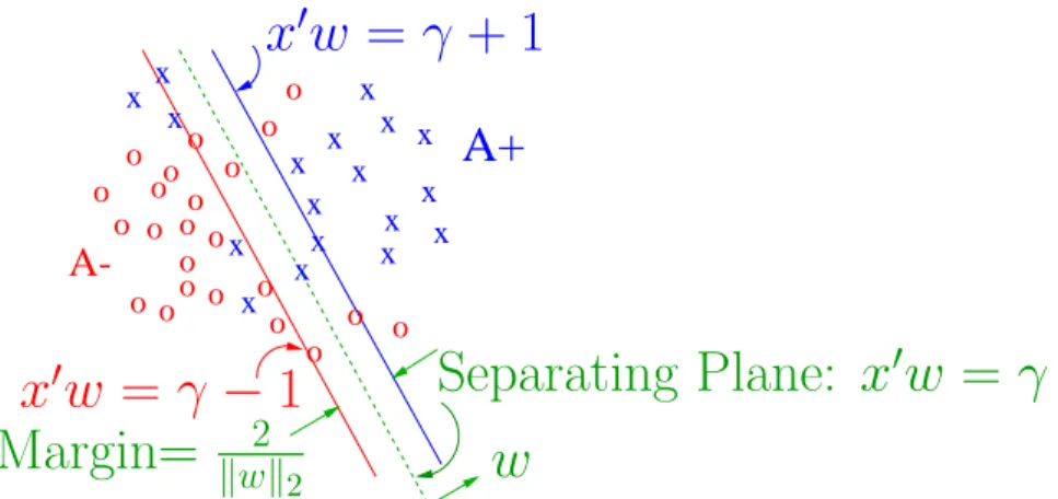
As was the case in [20], our recent active set support vector machine (ASVM) approach, the following two simple changes were made to the stan-dard linear SVM: (i) The margin (distance) between the parallel bounding planes was maximized with respect to both orientation (w) as well as location relative to the origin (γ). Such a change was also carried out in the succes-sive overrelaxation (SOR) approach of [19] as well as in the smooth support vector machine (SSVM) approach of [15]. See equation (7) and Figure 1. (ii) The error in the soft margin (y) was minimized using the 2-norm squared instead of the conventional 1-norm. See equation (7). These straightforward, but important changes, lead to a considerably simpler positive definite dual problem with nonnegativity constraints only. See equation (8). Although our use of a quadratic penalty for the soft margin as indicated in (ii) above is nonstandard, it has been used effectively in previous work [14, 13, 20]. In theory, this change could lead to a less robust classifier in the presence of outliers. However, this modification to the SVM does not seem to have a detrimental effect, as can be seen in the experimental results of Section 5.
In Section 2 of the paper we begin with the standard SVM formulation and its dual and then give our formulation and its dual. We note that com-putational evidence given in [20] shows that this alternative formulation does
not compromise on generalization ability. Section 3 gives our simple iterative Lagrangian support vector machine (LSVM) Algorithm 3.1 and establishes its global linear convergence. LSVM, stated in 11 lines of MATLAB Code 3.2 below, solves once at the outset a single system of n + 1 equations in
n+ 1 variables given by a symmetric positive definite matrix. It then uses a linearly convergent iterative method to solve the problem. In Section 4 LSVM is extended to positive semidefinite kernels. Section 5 describes our numerical results which show that LSVM gives comparable or better testing results than those of other SVM algorithms, and in some cases is dramatically faster than a standard quadratic programming SVM solver.
We now describe our notation and give some background material. All vectors will be column vectors unless transposed to a row vector by a prime 0.
For a vectorxin then-dimensional real spaceRn,x
+denotes the vector inRn
with all of its negative components set to zero. This corresponds to projecting
x onto the nonnegative orthant. The base of the natural logarithms will be denoted by ε , and for a vectory ∈Rm, ε−y will denote a vector in Rm with components ε−yi, i = 1, . . . , m. The notation A ∈ Rm×n will signify a real m×n matrix. For such a matrix A0 will denote the transpose of A, A
i will denote thei-th row of Aand A·j will denote thej-th column of A. A vector of ones or zeroes in a real space of arbitrary dimension will be denoted by e
or 0, respectively. The identity matrix of arbitrary dimension will be denoted by I. For two vectors x and y in Rn, x ⊥ y denotes orthogonality, that is
x0y = 0. We use := to denote definition. The 2-norm of a vector x and a
matrix Qwill be denoted by kxk and kQk respectively. A separating plane, with respect to two given point sets Aand BinRn, is a plane that attempts to separate Rn into two halfspaces such that each open halfspace contains points mostly ofA orB. A special case of the Sherman-Morrison-Woodbury (SMW) identity [8] will be utilized:
(I
ν +HH
0)−1 =ν(I −H(I ν +H
0H)−1H0), (1)
where ν is a positive number and H is an arbitrary m ×k matrix. This identity, easily verifiable by premultiplying both sides by (I
ν +HH
0), enables
us to invert a large m×m matrix of the form in (1) by merely inverting a smaller k×k matrix. It was also used recently in [20, 7].
2
The Linear Support Vector Machine
We consider the problem of classifying m points in the n-dimensional real space Rn, represented by the m×n matrix A, according to membership of each point Ai in the classA+ orA− as specified by a given m×mdiagonal matrix D with plus ones or minus ones along its diagonal. For this problem the standard support vector machine with a linear kernel [29, 5] is given by the following quadratic program with parameter ν >0:
min
(w,γ,y)∈Rn+1+mνe
0y+1
2w
0w s.t. D(Aw−eγ) +y≥e, y≥0. (2)
Here w is the normal to the bounding planes:
x0w=γ±1 (3)
and γ determines their location relative to the origin. See Figure 1. The planex0w=γ+ 1 bounds the class A+ points, possibly with some error, and
the plane x0w=γ−1 bounds the class A− points, also possibly with some
error. The linear separating surface is the plane:
x0w=γ, (4)
midway between the bounding planes (3). The quadratic term in (2) is twice the reciprocal of the square of the 2-norm distance 2/kwk2 between the two
bounding planes of (3) (see Figure 1). This term enforces maximization of this distance, which is often called the “margin”. If the classes are linearly inseparable, as depicted in Figure 1, then the two planes bound the two classes with a “soft margin”. That is, they bound each set approximately with some error determined by the nonnegative error variable y:
Aiw + yi ≥ γ+ 1, forDii= 1,
Aiw − yi ≤ γ−1, forDii =−1. (5) Traditionally the constant ν in (2) multiplies the the 1-norm of the error variable y and acts as a weighting factor. A nonzeroy results in an approxi-mate separation as depicted in Figure 1. The dual to the standard quadratic linear SVM (2) [16, 28, 17, 6] is the following:
min u∈Rm
1 2u
x x x x x x x x x x x
A+
A-o o o oo o o o o o o o o o o o o x x x o x o o o o o x x x PSfrag replacementsw
Margin=
kwk2 2x
0w
=
γ
−
1
x
0w
=
γ
+ 1
Separating Plane:
x
0w
=
γ
Figure 1: The bounding planes (3) with a soft (i.e. with some errors) margin
2
kwk2, and the plane (4) approximately separatingA+ fromA−.
The variables (w, γ) of the primal problem which determine the separating surface (4) can be obtained from the solution of the dual problem above [19, Eqns. 5 and 7]. We note immediately that the matrix DAA0D
ap-pearing in the dual objective function (6) is not positive definite in general because typically m >> n. Also, there is an equality constraint present, in addition to bound constraints, which for large problems necessitates special computational procedures such as SMO [26] or SVMlight [11]. Furthermore, a one-dimensional optimization problem [19] must be solved in order to de-termine the locator γ of the separating surface (4). In order to overcome all these difficulties as well as that of dealing with the necessity of having to essentially invert a very large matrix of the order of m×m, we propose the following simple but critical modifications to the standard SVM formu-lation (2). We change the 1-norm of y to a 2-norm squared which makes the constraint y ≥ 0 redundant. We also append the term γ2 to w0w. This
in effect maximizes the margin between the parallel separating planes (3) by optimizing with respect to both w and γ [19], that is with respect to both orientation and location of the planes, rather that just with respect to
w which merely determines the orientation of the plane. This leads to the following reformulation of the SVM:
min (w,γ,y)∈Rn+1+mν y0y 2 + 1 2(w 0w+γ2) s.t.D(Aw−eγ) +y ≥e. (7)
the dual of this problem is [16]: min 0≤u∈Rm 1 2u 0(I ν +D(AA 0+ee0)D)u−e0u. (8)
The variables (w, γ) of the primal problem which determine the separating surface (4) are recovered directly from the solution of the dual (8) above by the relations:
w=A0Du, y= u
ν, γ =−e
0Du. (9)
We immediately note that the matrix appearing in the dual objective function is positive definite and that there is no equality constraint and no upper bound on the dual variable u. The only constraint present is a nonnegativity one. These facts lead us to our simple iterative Lagrangian SVM Algorithm which requires the inversion of a positive definite (n+1)×(n+1) matrix, at the beginning of the algorithm followed by a straightforward linearly convergent iterative scheme that requires no optimization package.
3
LSVM (Lagrangian Support Vector Machine)
Algorithm
Before stating our algorithm we define two matrices to simplify notation as follows:
H =D[A −e], Q= I
ν +HH
0. (10)
With these definitions the dual problem (8) becomes min 0≤u∈Rmf(u) := 1 2u 0 Qu−e0u. (11)
It will be understood that within the LSVM Algorithm, the single time that
Q−1 is computed at the outset of the algorithm, the SMW identity (1) will
be used. Hence only an (n+ 1)×(n+ 1) matrix is inverted.
The LSVM Algorithm is based directly on the Karush-Kuhn-Tucker nec-essary and sufficient optimality conditions [16, KTP 7.2.4, page 94] for the dual problem (11):
0≤u ⊥ Qu−e≥0. (12)
By using the easily established identity between any two real numbers (or vectors) a and b:
the optimality condition (12) can be written in the following equivalent form for any positive α:
Qu−e= ((Qu−e)−αu)+. (14)
These optimality conditions lead to the following very simple iterative scheme which constitutes our LSVM Algorithm:
ui+1 =Q−1(e+ ((Qui−e)−αui)
+), i= 0,1, . . . , (15)
for which we will establish global linear convergence from any starting point under the easily satisfiable condition:
0< α < 2
ν. (16)
We impose this condition as α = 1.9/ν in all our experiments, where ν is the parameter of our SVM formulation (7). It turns out, and this is the way that led us to this iterative scheme, that the optimality condition (14), is also the necessary and sufficient condition for the unconstrained minimum of the implicit Lagrangian [22] associated with the dual problem (11):
min u∈RmL(u, α) = minu∈Rm 1 2u 0Qu−e0u+ 1 2α(k(−αu+Qu−e)+k 2 − kQu−ek2). (17) Setting the gradient with respect to u of this convex and differentiable La-grangian to zero gives
(Qu−e) + 1 α(Q−αI)((Q−αI)u−e)+− 1 αQ(Qu−e) = 0, (18) or equivalently: (αI −Q)((Qu−e)−((Q−αI)u−e)+) = 0, (19)
which is equivalent to the optimality condition (14) under the assumption that α is positive and not an eigenvalue of Q.
We establish now the global linear convergence of the iteration (15) under condition (16).
Algorithm 3.1 LSVM Algorithm & Its Global Convergence LetQ∈
Rm×m be the symmetric positive definite matrix defined by (10) and let (16)
hold. Starting with an arbitrary u0 ∈Rm, the iterates ui of (15) converge to
the unique solution u¯ of (11) at the linear rate:
Proof Because ¯u is the solution of (11), it must satisfy the optimality con-dition (14) for any α > 0. Subtracting that equation with u = ¯u from the iteration (15) premultiplied by Qand taking norms gives:
kQui+1−Qu¯k=k(Qui−e−αui)
+−(Qu¯−e−αu¯)+k (21)
Using the Projection Theorem [2, Proposition 2.1.3] which states that the distance between any two points in Rm is not less than the distance between their projections on any convex set (the nonnegative orthant here) in Rm, the above equation gives:
kQui+1−Qu¯k ≤ k(Q−αI)(ui−u¯)k
≤ kI−αQ−1k · kQ(ui−u¯)k. (22) All we need to show now is that kI−αQ−1k<1. This follows from (16) as
follows. Noting the definition (10) of Q and letting λi, i = 1, . . . , m, denote the nonnegative eigenvalues of HH0, all we need is:
−1<1−α(1 ν +λi) −1 <1, (23) or equivalently: 2> α(1 ν +λi) −1 >0, (24)
which is satisfied under the assumption (16).2
We give now a complete MATLAB [23] code of LSVM which is capable of solving problems with millions of points using only native MATLAB com-mands. The input parameters, besides A, D and ν of (10), which define the problem, are: itmax, the maximum number of iterations and tol, the toler-ated nonzero error in kui+1 −uik at termination. The quantity kui+1−uik bounds from above:
kQk−1· kQui−e−((Qui−e)−αui)
+k, (25)
which measures the violation of the optimality criterion (14). It follows by [21] thatkui+1−uikalso boundskui−u¯k, and by (9) it also bounds kwi−w¯k and |γi−γ¯|, where ( ¯w,¯γ,y¯) is the unique solution of the primal SVM (7).
Code 3.2 LSVM MATLAB Code
function [it, opt, w, gamma] = svml(A,D,nu,itmax,tol) % lsvm with SMW for min 1/2*u’*Q*u-e’*u s.t. u=>0, % Q=I/nu+H*H’, H=D[A -e]
% Input: A, D, nu, itmax, tol; Output: it, opt, w, gamma % [it, opt, w, gamma] = svml(A,D,nu,itmax,tol);
[m,n]=size(A);alpha=1.9/nu;e=ones(m,1);H=D*[A -e];it=0; S=H*inv((speye(n+1)/nu+H’*H));
u=nu*(1-S*(H’*e));oldu=u+1;
while it<itmax & norm(oldu-u)>tol
z=(1+pl(((u/nu+H*(H’*u))-alpha*u)-1)); oldu=u; u=nu*(z-S*(H’*z)); it=it+1; end; opt=norm(u-oldu);w=A’*D*u;gamma=-e’*D*u; function pl = pl(x); pl = (abs(x)+x)/2;
4
LSVM for Nonlinear Kernels
In this section of the paper we show how LSVM can be used to solve classifica-tion problems with positive semidefinite nonlinear kernels. Algorithm 3.1 and its convergence can be extended for such nonlinear kernels as we show below. The only price paid for this extension is that problems with large datasets can be handled using the Sherman-Morrison-Woodbury (SMW) identity (1) only if the inner product terms of the kernel [17, Equation (3)] are explicitly known, which in general they are not. Nevertheless LSVM may be a useful tool for classification with nonlinear kernels because of its extreme simplicity as we demonstrate below with the simple MATLAB code for which it does not make use of the Sherman-Morrison-Woodbury identity nor any optimization package.
We shall use the notation of [17]. ForA∈Rm×n andB ∈Rn×`, the ker-nel K(A, B) mapsRm×n×Rn×` intoRm×`. A typical kernel is the Gaussian kernel ε−µkA0
i−B·jk2, i, j = 1, . . . , m, ` = m, where ε is the base of natural
Rn, K(x0, A0) is a row vector inRm, and the linear separating surface (4) is replaced by the nonlinear surface
K([x0 −1], A0 −e0 )Du= 0, (26)
where u is the solution of the dual problem (11) with Q re-defined for a general nonlinear kernel as follows:
G= [A −e], Q= I
ν +DK(G, G
0)D. (27)
Note that the nonlinear separating surface (26) degenerates to the linear one (4) if we let K(G, G0) =GG0 and make use of (9).
To justify the nonlinear kernel formulation (27) we refer the reader to [17, Equation (8.9)] for a similar result and give a brief derivation here. If we rewrite our dual problem for a linear kernel (8) in the equivalent form:
min 0≤u∈Rm 1 2u 0(I ν +DGG 0D)u−e0u, (28)
and replace the linear kernelGG0 by a general nonlinear positive semidefinite
symmetric kernel K(G, G0) we obtain:
min 0≤u∈Rm 1 2u 0(I ν +DK(G, G 0)D)u−e0u. (29)
This is the formulation given above in (27). We note that the Karush-Kuhn-Tucker necessary and sufficient optimality conditions for this problem are:
0≤u ⊥ (I ν +DK([A −e], A0 −e0 )D)u−e≥0, (30) which underly LSVM for a nonlinear positive semidefinite kernel K(G, G0).
The positive semidefiniteness of the nonlinear kernel K(G, G0) is needed in
order to ensure the existence of a solution to both (29) and (30).
All the results of the previous section remain valid, with Q re-defined as above for any positive semidefinite kernel K. This includes the itera-tive scheme (15) and the convergence result given under the Algorithm 3.1. However, because we do not make use of the Sherman-Morrison-Woodbury identity for a nonlinear kernel, the LSVM MATLAB Code 3.2 is somewhat different and is as follows:
Code 4.1 LSVM MATLAB Code for Nonlinear Kernel K(·,·) function [it, opt,u] = svmlk(nu,itmax,tol,D,KM)
% lsvm with nonlinear kernel for min 1/2*u’*Q*u-e’*u s.t. u=>0 % Q=I/nu+DK(G,G’)D, G=[A -e]
% Input: nu, itmax, tol, D, KM=K(G,G’) % [it, opt,u] = svmlk(nu,itmax,tol,D,KM);
m=size(KM,1);alpha=1.9/nu;e=ones(m,1);I=speye(m);it=0; Q=I/nu+D*KM*D;P=inv(Q);
u=P*e;oldu=u+1;
while it<itmax & norm(oldu-u)>tol oldu=u; u=P*(1+pl(Q*u-1-alpha*u)); it=it+1; end; opt=norm(u-oldu);[it opt] function pl = pl(x); pl = (abs(x)+x)/2;
Since we cannot use the Sherman-Morrison-Woodbury identity in the general nonlinear case, we note that this code for a nonlinear kernel is effective for moderately sized problems. The sizes of the matrices P and Q in Code 4.1 scale quadratically with the number of data points.
5
Numerical Implementation and Comparisons
The implementation of LSVM is straightforward, as shown in the previous sections. Our first “dry run” experiments were on randomly generated prob-lems just to test the speed and effectiveness of LSVM on large probprob-lems. We first used a Pentium III 500 MHz notebook with 384 megabytes of memory (and additional swap space) on 2 million randomly generated points in R10
with ν = 1
m and α =
1.9
ν . LSVM solved the problem in 6 iterations in 81.52 minutes to an optimality criterion of 9.398e− 5 on a 2-norm violation of (14). The same problem was solved in the same number of iterations and to the same accuracy in 6.74 minutes on a 250 MHz UltraSPARC II processor with 2 gigabytes of memory. After these preliminary encouraging tests we proceeded to more systematic numerical tests as follows.
Most of the rest of our experiments were run on the Carleton College workstation “gray”, which utilizes a 700 MHz Pentium III Xeon processor and a maximum of 2 Gigabytes of memory available for each process. This computer runs Redhat Linux 6.2, with MATLAB 6.0. The one set of experi-ments showing the checkerboard were run on the UW-Madison Data Mining Institute “locop2” machine, which utilizes a 400 MHz Pentium II and a max-imum of 2 Gigabytes of memory available for each process. This computer runs Windows NT Server 4.0, with MATLAB 5.3.1. Both gray and locop2 are multiprocessor machines. However, only one processor was used for all the experiments shown here as MATLAB is a single threaded application and does not distribute any effort across processors. [1]. We had exclusive access to these machines, so there were no issues with other users inconsistently slowing the computers down.
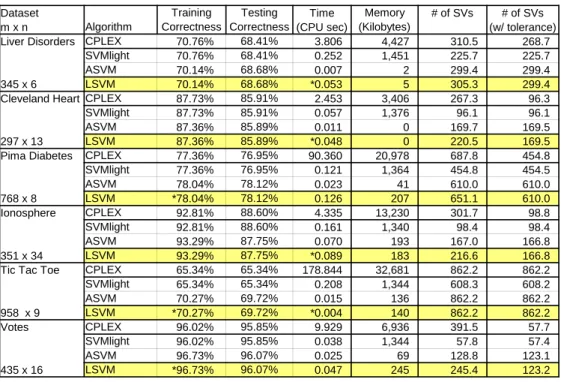
The first results we present are designed to show that our reformulation of the SVM (7) and its associated algorithm LSVM yield similar performance to the standard SVM (2), referred to here as SVM-QP. Results are also shown for our active set SVM (ASVM) algorithm which are described in [20]. For six datasets available from the UCI Machine Learning Repository [24], we performed tenfold cross validation in order to compare test set accuracies between the methodologies. Furthermore, we utilized a tuning set for each algorithm to find the optimal value of the parameter ν. For both LSVM and ASVM, we used an optimality tolerance of 0.001 to determine when to terminate. SVM-QP was implemented using the high-performing CPLEX barrier quadratic programming solver [10] with its default stopping criterion. Altering the CPLEX default stopping criterion to match that of LSVM did not result in significant change in timing relative to LSVM, but did reduce test set correctness for SVM-QP.
We also tested SVM-QP with the well-known SVM optimized algorithm SVMlight [11]. Joachims, the author of SVMlight, graciously provided us with the newest version of the software (Version 3.10b) and advice on setting the parameters. All features for all experiments were normalized to the range [−1,+1] as recommended in the SVMlight documentation. Such normaliza-tion was used in all experiments that we present, and is recommended for the LSVM algorithm due to the penalty on the bias parameter γ which we have added to our objective (7). We chose to use the default termination error criterion in SVMlight of 0.001. We also present an estimate of how much memory each algorithm used, as well as the number of support vec-tors. A support vector was determined here as the number of components of
Dataset Training Testing Time Memory # of SVs # of SVs m x n Algorithm Correctness Correctness (CPU sec) (Kilobytes) (w/ tolerance)
Liver Disorders CPLEX 70.76% 68.41% 3.806 4,427 310.5 268.7
SVMlight 70.76% 68.41% 0.252 1,451 225.7 225.7
ASVM 70.14% 68.68% 0.007 2 299.4 299.4
345 x 6 LSVM 70.14% 68.68% *0.053 5 305.3 299.4
Cleveland Heart CPLEX 87.73% 85.91% 2.453 3,406 267.3 96.3
SVMlight 87.73% 85.91% 0.057 1,376 96.1 96.1
ASVM 87.36% 85.89% 0.011 0 169.7 169.5
297 x 13 LSVM 87.36% 85.89% *0.048 0 220.5 169.5
Pima Diabetes CPLEX 77.36% 76.95% 90.360 20,978 687.8 454.8
SVMlight 77.36% 76.95% 0.121 1,364 454.8 454.5 ASVM 78.04% 78.12% 0.023 41 610.0 610.0 768 x 8 LSVM *78.04% 78.12% 0.126 207 651.1 610.0 Ionosphere CPLEX 92.81% 88.60% 4.335 13,230 301.7 98.8 SVMlight 92.81% 88.60% 0.161 1,340 98.4 98.4 ASVM 93.29% 87.75% 0.070 193 167.0 166.8 351 x 34 LSVM 93.29% 87.75% *0.089 183 216.6 166.8
Tic Tac Toe CPLEX 65.34% 65.34% 178.844 32,681 862.2 862.2
SVMlight 65.34% 65.34% 0.208 1,344 608.3 608.2 ASVM 70.27% 69.72% 0.015 136 862.2 862.2 958 x 9 LSVM *70.27% 69.72% *0.004 140 862.2 862.2 Votes CPLEX 96.02% 95.85% 9.929 6,936 391.5 57.7 SVMlight 96.02% 95.85% 0.038 1,344 57.8 57.4 ASVM 96.73% 96.07% 0.025 69 128.8 123.1 435 x 16 LSVM *96.73% 96.07% 0.047 245 245.4 123.2
Table 1: LSVM compared with conventional SVM-QP (CPLEX and SVMlight) and ASVM on six UCI datasets. LSVM test correctness is comparable to SVM-QP, with timing much faster than CPLEX and faster than or comparable to SVMlight. An asterisk in the first three columns indicates that the LSVM results are significantly different from SVMlight at significance level α= 0.05.
the dual vector uthat were nonzero. Moreover, we also present the number of components of u larger than 0.001 (referred to in the table as “SVs with tolerance”).
The results demonstrate that LSVM performs comparably to SVM-QP with respect to generalizability, and shows running times comparable to or better than SVMlight. LSVM and ASVM show nearly identical generalization performance, as they solve the same optimization problem. Any differences in generalization observed between the two are only due to different approx-imate solutions being found at termination. LSVM and ASVM usually run in roughly the same amount of time, though there are some cases where ASVM is noticeably faster than LSVM. Nevertheless, this is impressive per-formance on the part of LSVM, which is a dramatically simpler algorithm than ASVM, CPLEX, and SVMlight. LSVM utilizes significantly less memory than the SVM-QP algorithms as well, though it does require more support vectors than SVM-QP. We address this point in the conclusion.
Training CPU Iterations Test Set Memory # of SVs # of SVs Set Size Sec Accuracy (Kilobytes) (w/ tolerance)
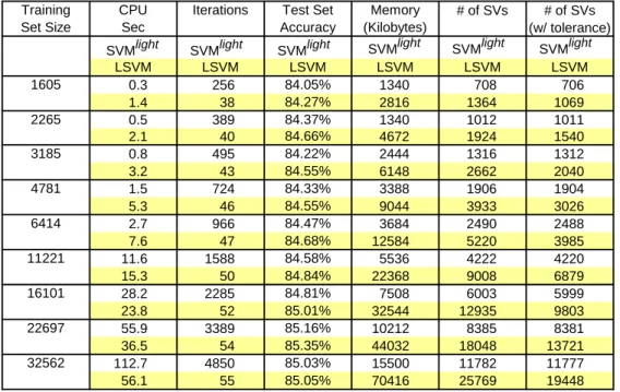
LSVM LSVM LSVM LSVM LSVM LSVM 1605 0.3 256 84.05% 1340 708 706 1.4 38 84.27% 2816 1364 1069 2265 0.5 389 84.37% 1340 1012 1011 2.1 40 84.66% 4672 1924 1540 3185 0.8 495 84.22% 2444 1316 1312 3.2 43 84.55% 6148 2662 2040 4781 1.5 724 84.33% 3388 1906 1904 5.3 46 84.55% 9044 3933 3026 6414 2.7 966 84.47% 3684 2490 2488 7.6 47 84.68% 12584 5220 3985 11221 11.6 1588 84.58% 5536 4222 4220 15.3 50 84.84% 22368 9008 6879 16101 28.2 2285 84.81% 7508 6003 5999 23.8 52 85.01% 32544 12935 9803 22697 55.9 3389 85.16% 10212 8385 8381 36.5 54 85.35% 44032 18048 13721 32562 112.7 4850 85.03% 15500 11782 11777 56.1 55 85.05% 70416 25769 19448 SVMlight SVMlight SVMlight SVMlight SVMlight SVMlight
Table 2: Comparison of LSVM with SVMlight on the UCI adult dataset. LSVM test correctness is comparable to that of SVMlight, but is faster on large datasets. (ν= 0.03)
# of # of Training Testing Time Memory Points Attributes Iterations Correctness Correctness (CPU min) (Kilobytes)
2 million 10 81 69.80% 69.44% 22.4 918,256
Table 3: Performance of LSVM on NDC [25] generated dataset (ν = 0.1).
SVMlight failed on this dataset.
We next compare LSVM with SVMlighton the Adult dataset [24], which is commonly used to compare SVM algorithms [27, 19]. These results, shown in Table 2, demonstrate that for the largest training sets LSVM performs faster than SVMlight with similar test set accuracies. Note that the “it-erations” column takes on very different meanings for the two algorithms. SVMlight defines an iteration as solving an optimization problem over a a small number, or “chunk,” of constraints. LSVM, on the other hand, de-fines an iteration as a matrix calculation which updates all the dual variables simultaneously. These two numbers are not directly comparable, and are included here only for purposes of monitoring scalability. In this experiment, LSVM uses significantly more memory than SVMlight.
Table 3 shows results from running LSVM on a massively sized dataset. This dataset was created using our own NDC Data Generator [25] as sug-gested by Usama Fayyad. The results show that LSVM can be used to solve massive problems quickly, which is particularly intriguing given the simplic-ity of the LSVM Algorithm. Note that for these experiments, all the data was brought into memory. As such, the running time reported consists of the time used to actually solve the problem to termination excluding I/O time. This is consistent with the measurement techniques used by other popular approaches [11, 26]. Putting all the data in memory is simpler to code and results in faster running times. However, it is not a fundamental requirement of our algorithm — block matrix multiplications, incremental evaluations of
Q−1 using another application of the Sherman-Morrison-Woodbury identity,
and indices on the dataset can be used to create an efficient disk based ver-sion of LSVM. We note that we tried to run SVMlight on this dataset, but after running for more than six hours it did not terminate.
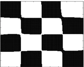
We now demonstrate the effectiveness of LSVM in solving nonlinear classi-fication problems through the use of kernel functions. One highly nonlinearly separable but simple example is the “tried and true” checkerboard dataset [9], which has often been used to show the effectiveness of nonlinear kernel methods on a dataset for which a linear separation clearly fails. The checker-board dataset contains 1000 points randomly sampled from a checkerchecker-board.
−100 −80 −60 −40 −20 0 20 40 60 80 100 −100 −80 −60 −40 −20 0 20 40 60 80 100
Figure 2: Gaussian kernel LSVM performance on checkerboard training dataset. (ν= 105)
These points are used as a training set in LSVM to try to reproduce an ac-curate rendering of a checkerboard. For this problem, we used the following Gaussian kernel:
K(G, G0) = exp(−2·10−4kGi0 −G·jk22), i, j = 1, . . . , m (31)
Our results, shown in Figure 2, demonstrate that LSVM shows similar or better generalization capability on this dataset when compared to other methods [12, 18, 15]. Total time for the checkerboard problem using LSVM with a Gaussian kernel was 2.85 hours on the Locop2 Pentium II Xeon ma-chine on the 1000-point training set in R2 after 100,000 iterations. Test
set accuracy was 97.0% on a 39,000-point test set. However, within 58 sec-onds and after 100 iterations, a quite reasonable checkerboard was obtained (www.cs.wisc.edu/~olvi/lsvm/check100iter.eps) with a 95.9% accuracy on the same test set.
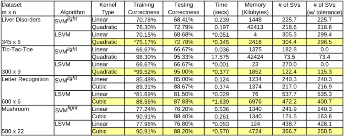
The final set of experiments, shown in Table 4, demonstrates the ef-fectiveness of nonlinear kernel functions with LSVM on UCI datasets [24] specialized as follows for purposes of our tests:
• The liver-disorders dataset contains 345 points, each consisting of six features. Class 1 contains 145 points, and class -1 contains 200 points.
• The letter-recognition dataset is used for recognizing letters of the al-phabet. Traditionally, this dataset is used for multi-category classifi-cation. We used it here in a two class situation by taking a subset of those points which correspond to the letter “A,” and a subset of those points which correspond to the letter “B.” This resulted in a dataset of 600 points with 6 features, where each class contained 300 points. • The mushroomdataset is a two class dataset which contains eight
cat-egorical attributes. We transformed each catcat-egorical attribute into a series of binary attributes, one attribute for each distinct value. For example, this dataset contains an attribute called “cap surface,” which can take one one of four categories, namely “fibrous,” “grooves,” “scaly,” or “smooth.” We represented this as four binary attributes. A 1 is assigned to the attribute that corresponds to the actual category, and a 0 to the rest. Thus the categorical value “fibrous” would be rep-resented by [1 0 0 0], while the value “smooth” would be reprep-resented by [0 0 0 1]. A subset of the entire mushroom dataset was used, so as to shorten the running times of our experiments. The final dataset we used contained 22 features with 200 points in class 1 and 300 points in class -1.
• The tic-tac-toe dataset is a two class dataset that contains incomplete tic-tac-toe games. All those games with a possible winning move for “X” end up in category 1, and all other games end up in category -1. We have intentionally represented this problem with a poor represen-tation scheme to show the power of non-linear kernels in overcoming this difficulty. Each tic-tac-toe game is represented by 9 attributes, where each attribute corresponds to a spot on the tic-tac-toe board. An “X” is represented by 1, an “O” is represented by 0, and a blank is represented by -1. We used a subset of this dataset with 9 attributes, 200 points in class 1, and 100 points in class -1.
We chose which kernels to use and appropriate values of ν via tuning sets and tenfold cross-validation techniques. The results show that nonlinear kernels produce test set accuracies that improve on those obtained with linear kernels.
Dataset Kernel Training Testing Time Memory # of SVs # of SVs m x n Algorithm Type Correctness Correctness (secs) (Kilobytes) (w/ tolerance)
Liver Disorders Linear 70.76% 68.41% 0.239 1448 225.7 225.7
Quadratic 76.30% 72.79% 0.197 42413 218.6 218.6 LSVM Linear 70.15% 68.68% *0.051 4 305.3 299.4 345 x 6 Quadratic *75.17% 72.78% *0.345 2418 304.4 298.5 Tic-Tac-Toe Linear 66.67% 66.67% 0.036 1375 182.8 0.0 Quadratic 98.30% 95.33% 17.575 42424 73.5 73.4 LSVM Linear 66.67% 66.67% *0.001 23 270.0 0.0 300 x 9 Quadratic *99.52% 95.00% *0.377 1852 122.4 115.3
Letter Recognition Linear 85.48% 85.00% 0.124 1234 240.3 240.3
Cubic 89.31% 88.67% 0.374 1374 217.0 216.9 LSVM Linear *81.69% 81.50% *0.029 76 537.7 535.3 600 x 6 Cubic 88.56% 87.83% *1.639 6976 472.2 400.7 Mushroom Linear 77.24% 76.20% 0.536 1340 241.9 240.3 Cubic 90.91% 88.40% 0.261 1340 174.5 163.6 LSVM Linear 77.96% 76.80% *0.053 124 438.7 428.1 500 x 22 Cubic 90.91% 88.20% *0.570 4724 366.7 250.5 SVMlight SVMlight SVMlight SVMlight
Table 4: LSVM performance with linear, quadratic, and cubic kernels (poly-nomial kernels of degree 1, 2, and 3 respectively). An asterisk in the first three columns indicates that the LSVM results are significantly different from SVMlight at significance level α= 0.05.
6
Conclusion
A fast and extremely simple algorithm, LSVM, considerably easier to code than SVMlight [11], SMO [27], SOR [19] and ASVM [20], capable of classify-ing datasets with millions of points has been proposed and implemented in a few lines of MATLAB code. For a linear kernel LSVM is an iterative method which requires nothing more complex than the inversion of a single matrix of the order of the input space plus one and thus has the ability to handle massive problems. For a positive semidefinite nonlinear kernel a single ma-trix inversion is required in the space of dimension equal to the number of points classified. Hence for such nonlinear classifiers LSVM can handle only intermediate size problems.
There is room for future work in reducing the number of support vectors in the solutions yielded by LSVM. One method would be to augment the quadratic term in y in the objective function of (7) by a 1-norm in y. This should decrease the number of support vectors as in [3] where the 1-norm was used to effectively suppress features. Additionally, the iterative algorithm itself could be modified so that dual variables with values smaller than a tolerance would be automatically set to zero.
Further future work includes extensions to parallel processing of the data and handling very large datasets directly from disk as well as extending nonlinear kernel classification to very large datasets.
Acknowledgements
Research described in this Data Mining Institute Report 00-06, June 2000, was supported by National Science Foundation Grants CCR-9729842 and CDA-9623632, by Air Force Office of Scientific Research Grant F49620-00-1-0085 and by Microsoft. We wish to thank our colleague Thorsten Joachims for supplying us with his latest code for SVMlight and for advice on how to run it efficiently.
c
2000 Olvi L. Mangasarian and David R. Musicant.
The LSVM Algorithm 3.1 and the LSVM Codes 3.2 and 4.1 are copyrighted and may not be used for any commercial purpose without written authoriza-tion from the authors.
References
[1] Matlab solution number 1913: Can one session of matlab take advan-tage of multiple processors on the same pc or unix machine?, 2000. http://www.mathworks.com/support/solutions/data/1913.shtml. [2] D. P. Bertsekas. Nonlinear Programming. Athena Scientific, Belmont,
MA, second edition, 1999.
[3] P. S. Bradley and O. L. Mangasarian. Feature selection via concave min-imization and support vector machines. In J. Shavlik, editor, Machine Learning Proceedings of the Fifteenth International Conference(ICML ’98), pages 82–90, San Francisco, California, 1998. Morgan Kaufmann. ftp://ftp.cs.wisc.edu/math-prog/tech-reports/98-03.ps.
[4] P. S. Bradley and O. L. Mangasarian. Massive data discrimination via linear support vector machines. Optimization Methods and Software, 13:1–10, 2000. ftp://ftp.cs.wisc.edu/math-prog/tech-reports/98-03.ps. [5] V. Cherkassky and F. Mulier. Learning from Data - Concepts, Theory
and Methods. John Wiley & Sons, New York, 1998.
[6] N. Cristianini and J. Shawe-Taylor. An Introduction to Support Vector Machines. Cambridge University Press, Cambridge, 2000.
[7] M. C. Ferris and T. S. Munson. Interior point methods for massive support vector machines. Technical Report 00-05, Computer Sciences Department, University of Wisconsin, Madison, Wisconsin, May 2000. ftp://ftp.cs.wisc.edu/pub/dmi/tech-reports/00-05.ps.
[8] G. H. Golub and C. F. Van Loan. Matrix Computations. The John Hopkins University Press, Baltimore, Maryland, 3rd edition, 1996. [9] T. K. Ho and E. M. Kleinberg. Checkerboard dataset, 1996.
http://www.cs.wisc.edu/math-prog/mpml.html.
[10] ILOG CPLEX Division, Incline Village, Nevada. ILOG CPLEX 6.5 Reference Manual, 1999.
[11] T. Joachims. SVMlight, 1998. http://www-ai.informatik. uni-dortmund.de/FORSCHUNG/VERFAHREN/SVM_LIGHT/svm_light. eng.html.
[12] L. Kaufman. Solving the quadratic programming problem arising in support vector classification. In B. Sch¨olkopf, C. J. C. Burges, and A. J. Smola, editors, Advances in Kernel Methods - Support Vector Learning, pages 147–167. MIT Press, 1999.
[13] Y.-J. Lee and O. L. Mangasarian. RSVM: Reduced support vector ma-chines. Technical Report 00-07, Data Mining Institute, Computer Sci-ences Department, University of Wisconsin, Madison, Wisconsin, July 2000. ftp://ftp.cs.wisc.edu/pub/dmi/tech-reports/00-07.ps.
[14] Yuh-Jye Lee and O. L. Mangasarian. SSVM: A smooth support vec-tor machine. Technical Report 99-03, Data Mining Institute, Com-puter Sciences Department, University of Wisconsin, Madison, Wiscon-sin, September 1999. Computational Optimization and Applications, to appear. ftp://ftp.cs.wisc.edu/pub/dmi/tech-reports/99-03.ps.
[15] Yuh-Jye Lee and O. L. Mangasarian. SSVM: A smooth support vec-tor machine. Computational Optimization and Applications, 2000. To appear. ftp://ftp.cs.wisc.edu/pub/dmi/tech-reports/99-03.ps.
[16] O. L. Mangasarian. Nonlinear Programming. SIAM, Philadelphia, PA, 1994.
[17] O. L. Mangasarian. Generalized support vector machines. In A. Smola, P. Bartlett, B. Sch¨olkopf, and D. Schuurmans, editors, Advances in Large Margin Classifiers, pages 135–146, Cambridge, MA, 2000. MIT Press. ftp://ftp.cs.wisc.edu/math-prog/tech-reports/98-14.ps.
[18] O. L. Mangasarian and D. R. Musicant. Data discrimination via nonlin-ear generalized support vector machines. Technical Report 99-03, Com-puter Sciences Department, University of Wisconsin, Madison, Wiscon-sin, March 1999. To appear in: “Applications and Algorithms of Com-plementarity”, M. C. Ferris, O. L. Mangasarian and J.-S. Pang, editors, Kluwer Academic Publishers,Boston 2000. ftp://ftp.cs.wisc.edu/math-prog/tech-reports/99-03.ps.
[19] O. L. Mangasarian and D. R. Musicant. Successive overrelaxation for support vector machines. IEEE Transactions on Neural Networks, 10:1032–1037, 1999. ftp://ftp.cs.wisc.edu/math-prog/tech-reports/98-18.ps.
[20] O. L. Mangasarian and D. R. Musicant. Active support vector machine classification. Technical Report 00-04, Data Mining Institute, Com-puter Sciences Department, University of Wisconsin, Madison, Wiscon-sin, April 2000. ftp://ftp.cs.wisc.edu/pub/dmi/tech-reports/00-04.ps. [21] O. L. Mangasarian and J. Ren. New improved error bounds for the
linear complementarity problem. Mathematical Programming, 66:241– 255, 1994.
[22] O. L. Mangasarian and M. V. Solodov. Nonlinear complementarity as unconstrained and constrained minimization. Mathematical Program-ming, Series B, 62:277–297, 1993.
[23] MATLAB. User’s Guide. The MathWorks, Inc., Natick, MA 01760, 1992.
[24] P. M. Murphy and D. W. Aha. UCI repository of machine learning databases, 1992. www.ics.uci.edu/∼mlearn/MLRepository.html.
[25] D. R. Musicant. NDC: normally distributed clustered datasets, 1998. www.cs.wisc.edu/∼musicant/data/ndc/.
[26] J. Platt. Sequential minimal optimization: A fast algorithm for train-ing support vector machines. In Sch¨olkopf et al. [28], pages 185–208. http://www.research.microsoft.com/∼jplatt/smo.html.
[27] J. Platt. Sequential minimal optimization: A fast algorithm for training support vector machines. In B. Sch¨olkopf, C. J. C. Burges, and A. J. Smola, editors, Advances in Kernel Meth-ods - Support Vector Learning, pages 185–208. MIT Press, 1999. http://www.research.microsoft.com/∼jplatt/smo.html.
[28] B. Sch¨olkopf, C. Burges, and A. Smola (editors). Advances in Kernel Methods: Support Vector Machines. MIT Press, Cambridge, MA, 1998. [29] V. N. Vapnik. The Nature of Statistical Learning Theory. Springer, New
![Table 3: Performance of LSVM on NDC [25] generated dataset (ν = 0.1).](https://thumb-us.123doks.com/thumbv2/123dok_us/9723232.2853884/15.918.167.746.187.269/table-performance-lsvm-ndc-generated-dataset-ν.webp)